Measurements of $J/\psi$ decays into $\phi\pi^{0}$, $\phi\eta$, and $\phi\eta^{\prime}$

Abstract

Based on $5.8\times 10^{7}J/\psi$ events detected in BESII, the branching fractions of $J/\psi\to\phi\eta$ and $\phi\eta^{\prime}$ are measured for different $\eta$ and $\eta^{\prime}$ decay modes. The results are significantly higher than previous measurements. An upper limit on $B(J/\psi\rightarrow\phi\pi^{0})$ is also obtained.

I Introduction

The decay of the $J/\psi$ into a vector and pseudoscalar meson pair, $J/\psi\to VP$ with $V$ and $P$ representing vector and pseudoscalar mesons, can proceed via strong and electromagnetic reactions. A well measured set of all possible decays of $J/\psi\to VP$ allows one to systematically study the quark gluon contents of pseudoscalar mesons, SU(3) breaking, as well as determine the electromagnetic and doubly suppressed OZI amplitudes in two-body $J/\psi$ decays theory . MARKIII mark2 ; mark3 and DM2 dm2 measured many $J/\psi\to VP$ decays and obtained the $\eta-\eta^{\prime}$ mixing angle, the quark content of the $\eta$ and $\eta^{\prime}$, and much more.

Recently, a sample of $5.8\times 10^{7}J/\psi$ events was accumulated with the upgraded Beijing Spectrometer (BESII) besii , which offers a unique opportunity to measure precisely the full set of $J/\psi\to VP$ decays. In an earlier analysis based on this data set, the branching fraction of $J/\psi\rightarrow\pi^{+}\pi^{-}\pi^{0}$ was measured to be $(2.10\pm 0.12)\%$ besrhopi , which is higher than the PDG pdg2004 value by about 30%. This indicates a higher branching fraction for $J/\psi\rightarrow\rho\pi$ than those from older experiments frhopi , since the dominant dynamics in $J/\psi\to\pi^{+}\pi^{-}\pi^{0}$ is $J/\psi\rightarrow\rho\pi$. Therefore, remeasuring the branching fractions of all $J/\psi\rightarrow VP$ decay modes becomes very important. In this paper, $J/\psi\to\phi\pi^{0}$, $\phi\eta$, and $\phi\eta^{\prime}$ are studied, based on the BESII $5.8\times 10^{7}J/\psi$ events.

II The BES Detector

The upgraded Beijing Spectrometer detector (BESII) is located at the Beijing Electron-Positron Collider (BEPC). BESII is a large solid-angle magnetic spectrometer which is described in detail in Ref. besii . The momentum of charged particles is determined by a 40-layer cylindrical main drift chamber (MDC) which has a momentum resolution of $\sigma_{p}$/p=$1.78\%\sqrt{1+p^{2}}$ ($p$ in GeV/c). Particle identification is accomplished using specific ionization ($dE/dx$) measurements in the drift chamber and time-of-flight (TOF) information in a barrel-like array of 48 scintillation counters. The $dE/dx$ resolution is $\sigma_{dE/dx}\simeq 8.0\%$; the TOF resolution for Bhabha events is $\sigma_{TOF}=180$ ps. Radially outside of the time-of-flight counters is a 12-radiation-length barrel shower counter (BSC) comprised of gas proportional tubes interleaved with lead sheets. The BSC measures the energy and direction of photons with resolutions of $\sigma_{E}/E\simeq 21\%\sqrt{E}$ ($E$ in GeV), $\sigma_{\phi}=7.9$ mrad, and $\sigma_{z}=2.3$ cm. The iron flux return of the magnet is instrumented with three double layers of proportional counters (MUC) that are used to identify muons.

A GEANT3 based Monte Carlo package (SIMBES) with detailed consideration of the detector performance is used. The consistency between data and Monte Carlo has been carefully checked in many high purity physics channels, and the agreement is reasonable. The detection efficiency and mass resolution for each decay mode are obtained from a Monte Carlo simulation which takes into account the angular distributions appropriate for the different final states rhopi .

III analysis

In this analysis, the $\phi$ meson is observed in its $K^{+}K^{-}$ decay mode, and the pseudoscalar mesons are detected in the modes: $\pi^{0}\rightarrow\gamma\gamma$; $\eta\rightarrow\gamma\gamma$, $\gamma\pi^{+}\pi^{-}$, and $\pi^{+}\pi^{-}\pi^{0}$; and $\eta^{\prime}\rightarrow\gamma\gamma$, $\gamma\pi^{+}\pi^{-}(\gamma\rho)$, and $\pi^{+}\pi^{-}\eta~{}(\eta\rightarrow\gamma\gamma)$. Using multiple $\eta$ and $\eta^{\prime}$ decay modes allows us to crosscheck our measurements, as well as obtain higher precision. Possible final states of $J/\psi\rightarrow\phi\pi^{0},~{}\phi\eta$, and $\phi\eta^{\prime}$ are then $K^{+}K^{-}\gamma\gamma$, $K^{+}K^{-}\pi^{+}\pi^{-}\gamma$, and $K^{+}K^{-}\pi^{+}\pi^{-}\gamma\gamma$. Candidate events are required to satisfy the following common selection criteria:

1. The events must have the correct number of charged tracks with net charge zero. Each track must be well fitted to a helix, originating from the interaction region of R${}_{xy}<$0.02 m and $|z|<$ 0.2 m, and have a polar angle, $\theta$, in the range $|\cos\theta|<$ 0.8.

2. Events should have at least the minimum number of isolated photons associated with the different final states. Isolated photons are those that have energy deposited in the BSC greater than 60 MeV, the angle between the direction at the first hit layer of the BSC and the developing direction of the cluster less than 30^∘, and the angle between photons and any charged tracks larger than 10^∘.

3. For each charged track in an event, $\chi^{2}_{PID}(i)$ is determined using both $dE/dx$ and TOF information:

   $\chi^{2}_{PID}(i)$=$\chi^{2}_{dE/dx}(i)$+$\chi^{2}_{TOF}(i)$

   A charged track is identified as a $\pi$ or $K$ if its $\chi^{2}_{PID}$ is less than those for any other assignment. To reject background events, two charged tracks are required to be identified as kaons in $J/\psi\rightarrow\phi\pi^{0}$. For the other channels, at least one charged track must be identified as a kaon in the event selection.

4. The selected events are fitted kinematically. The kinematic fit adjusts the track energy and momentum within the measured errors so as to satisfy energy and momentum conservation for the given event hypothesis. This improves resolution, selects the correct charged-particle assignment for the tracks, and reduces background. When the number of photons in an event exceeds the minimum, all combinations are tried, and the combination with the smallest $\chi^{2}$ is retained.

The branching fraction is calculated using

$$B(J/\psi\rightarrow\phi P)=$$

$$\frac{N_{obs}}{N_{J/\psi}\cdot\varepsilon\cdot B(\phi\rightarrow K^{+}K^{-})\cdot B(P\rightarrow X)},$$

where $N_{obs}$ is the number of events observed (or the upper limit), $N_{J/\psi}$ is the number of $J/\psi$ events, $(5.77\pm 0.27)\times 10^{7}$, determined from the number of inclusive 4-prong hadronic decays fangss , $\varepsilon$ is the detection efficiency obtained from Monte Carlo simulation, and $B(\phi\rightarrow K^{+}K^{-})$ and $B(P\rightarrow X)$ are the branching fractions of $\phi\rightarrow K^{+}K^{-}$ and pseudoscalar decays from the PDG pdg2004 , respectively.

III.1 $J/\psi\rightarrow\phi\gamma\gamma$

Events with two oppositely charged tracks and at least two or three isolated photons are selected. A 4C-fit is performed to the $K^{+}K^{-}\gamma\gamma$ hypothesis, and $\chi^{2}<15$ is required. To reject possible background events from $J/\psi\rightarrow\gamma K^{+}K^{-}\pi^{0}$, the 4C-fit probability for the assignment $J/\psi\rightarrow K^{+}K^{-}\gamma\gamma$ must be larger than that of $K^{+}K^{-}\gamma\gamma\gamma$.

After this selection, the scatter plot (Figure 1) of $m_{K^{+}K^{-}}$ versus $m_{\gamma\gamma}$ shows two clusters corresponding to $\phi\eta^{\prime}$ and $\phi\eta$, but there is no clear accumulation of events for $\phi\pi^{0}$. To obtain the $m_{\gamma\gamma}$ distribution recoiling against $\phi$, the $K^{+}K^{-}$ invariant mass is required to be in the $\phi$ mass region, $|m_{K^{+}K^{-}}-1.02|<0.02$ GeV/c².

Figure 1: Scatter plot of $m_{K^{+}K^{-}}$ versus $m_{\gamma\gamma}$ for $J/\psi\rightarrow K^{+}K^{-}\gamma\gamma$ events.

III.1.1 $J/\psi\rightarrow\phi\pi^{0}$

Figure 2(a) shows the $m_{\gamma\gamma}$ invariant mass distribution after the above selection; no clear $\pi^{0}$ signal is observed. The Bayesian method is used to determine the upper limit on the $J/\psi\rightarrow\phi\pi^{0}$ branching fraction. A Breit-Wigner convoluted with a Gaussian plus a polynomial background function are used to fit the $m_{\gamma\gamma}$ spectrum. The $\pi^{0}$ mass and width are fixed to PDG values. The mass resolution, obtained from Monte Carlo simulation, is 17.7 MeV/c². At the 90% confidence level, the number of $\phi\pi^{0}$ events is 24. Taking into account the detection efficiency, $(16.63\pm 0.20)\%$, the upper limit on the branching fraction is

$B(J/\psi\rightarrow\phi\pi^{0})<5.10\times 10^{-6}$

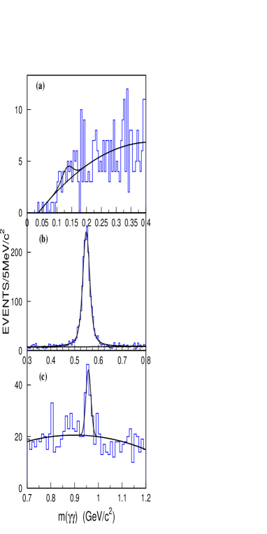
Figure 2: The invariant mass distribution of $m_{\gamma\gamma}$ for $J/\psi\rightarrow\phi\gamma\gamma$ events. The curves are the results of the fit described in the text.

III.1.2 $J/\psi\rightarrow\phi\eta$

Figure 2(b) shows the $m_{\gamma\gamma}$ distribution; an $\eta$ signal is clearly seen. The fit of this distribution with a Breit-Wigner convoluted with a Gaussian plus a second order polynomial background function gives $2086\pm 42$ $\phi\eta$ events with a $\eta$ mass of $549.0\pm 0.5$ MeV/c². The background events, $152\pm 17$, are estimated from the $\phi$ sidebands, defined by 0.98 GeV/c${}^{2}<m_{K^{+}K^{-}}<1.00$ GeV/c² and 1.04 GeV/c${}^{2}<m_{K^{+}K^{-}}<1.06$ GeV/c². After subtracting background and correcting for detection efficiency, $(19.98\pm 0.22)$%, the $J/\psi\rightarrow\phi\eta$ branching fraction is obtained

$B(J/\psi\rightarrow\phi\eta)=(8.67\pm 0.19)\times 10^{-4}$,

where the error is statistical only.

III.1.3 $J/\psi\rightarrow\phi\eta^{\prime}$

The distribution of $m_{\gamma\gamma}$ in $\eta^{\prime}$ mass region recoiling against the $\phi$ is shown in Figure 2(c). A fit of the $\eta^{\prime}$ peak with a Breit-Wigner and a second order backgound polynomial yields $68\pm 15$ $\phi\eta^{\prime}$ events with the peak at $958.1\pm 2.6$ MeV/c². No obvious signal is observed for the distribution of $m_{\gamma\gamma}$ recoiling against $\phi$ sidebands (0.98 GeV/c${}^{2}<m_{K^{+}K^{-}}<1.0$ GeV/c² and 1.04 GeV/c${}^{2}<m_{K^{+}K^{-}}<1.06$ GeV/$c^{2}$). The detection efficiency is $(18.57\pm 0.22)\%$, and the corresponding branching fraction is determined to be

$B(J/\psi\rightarrow\phi\eta^{\prime})=(6.10\pm 1.34)\times 10^{-4}$,

where the error is only the statistical error.

III.2 $J/\psi\rightarrow\phi\gamma\pi^{+}\pi^{-}$

For $J/\psi\to\phi\eta$, $\eta\to\gamma\pi^{+}\pi^{-}$, events with four well-reconstructed charged tracks and at least one isolated photon are required. To select the pions and kaons from amongst the tracks, 4C fits are applied for one of the following three cases: (1) if only one charged track is identified as a kaon using particle identification, then the other charged tracks are assumed, one at a time, to be a kaon, while the other two are assumed to be pions; (2) if two charged tracks are identified as kaons, then the other two tracks are assumed to be pions; (3) if three or four charged tracks are identified as kaons, then the particle identification information is ignored and all combinations of two kaon and two pion tracks are kinematicaly fitted. For each case, the hypothesis with the smallest $\chi^{2}$ is selected. We further require that the probability of the 4C fit for the $J/\psi\rightarrow K^{+}K^{-}\pi^{+}\pi^{-}\gamma$ assignment is larger than those of $K^{+}K^{-}\pi^{+}\pi^{-}$ and $K^{+}K^{-}\pi^{+}\pi^{-}\gamma\gamma$.

The scatter plot of $m_{K^{+}K^{-}}$ versus $m_{\gamma\pi^{+}\pi^{-}}$ is shown in Figure 3, where $J/\psi\rightarrow\phi\eta$ and $J/\psi\rightarrow\phi\eta^{\prime}$ decays are apparent. For the scatter plot of $m_{\pi^{+}\pi^{-}}$ versus $m_{\gamma\pi^{+}\pi^{-}}$, shown in Figure 4, the $\eta^{\prime}$ - $\rho$ signal corresponds to the decay $\eta^{\prime}\rightarrow\gamma\rho$. The other cluster is from $\eta\rightarrow\gamma\pi^{+}\pi^{-}$ and $\eta\rightarrow\pi^{0}\pi^{+}\pi^{-}$ background events.

Figure 3: Scatter plot of $m_{K^{+}K^{-}}$ versus $m_{\gamma\pi^{+}\pi^{-}}$ for $J/\psi\rightarrow K^{+}K^{-}\pi^{+}\pi^{-}\gamma$ events. The band below the $\eta$ signal comes from $\eta\rightarrow\pi^{+}\pi^{-}\pi^{0}$ events.

Figure 4: Scatter plot of $m_{\pi^{+}\pi^{-}}$ versus $m_{\gamma\pi^{+}\pi^{-}}$ for $J/\psi\rightarrow\phi\gamma\pi^{+}\pi^{-}$ events. The $\eta^{\prime}$ - $\rho$ signal corresponds to the decay $\eta^{\prime}\rightarrow\gamma\rho$. The other cluster is from $\eta\rightarrow\gamma\pi^{+}\pi^{-}$ and $\eta\rightarrow\pi^{0}\pi^{+}\pi^{-}$ background events.

III.2.1 $J/\psi\rightarrow\phi\eta$

Figure 5 shows the $\gamma\pi^{+}\pi^{-}$ invariant mass recoiling against the $\phi$, defined by $|m_{K^{+}K^{-}}-1.02|<0.02$ GeV/c². A clear $\eta$ signal is observed. The peak on the left side of the $\eta$ in Figure 5 comes from $J/\psi\rightarrow\phi\eta~{}(\eta\rightarrow\pi^{+}\pi^{-}\pi^{0})$ with one photon missing; this is confirmed by Monte-Carlo simulation. This peak cannot be described by a simple Breit-Wigner due to its asymmetric shape. To obtain the shape of the peak, a Monte-carlo sample of $J/\psi\rightarrow\phi\eta~{}(\eta\rightarrow\pi^{+}\pi^{-}\pi^{0})$ is generated and a fit is made to the peak. The $\gamma\pi^{+}\pi^{-}$ mass distribution is then fitted with this shape, a Breit-Wigner to describe the $\eta$ signal, and a polynomial background. The fit, shown in Figure 5, yields $134\pm 14$ $\eta$ events with a mass at $548.9\pm 0.9$ MeV/c². The detection efficiency obtained from Monte Carlo simulation is $(10.32\pm 0.16)\%$, and the corresponding branching fraction is

$B(J/\psi\rightarrow\phi\eta)=(9.79\pm 1.02)\times 10^{-4},$

where the error is only the statistical error.

Figure 5: Distribution of $m_{\gamma\pi^{+}\pi^{-}}$ for $J/\psi\rightarrow\phi\pi^{+}\pi^{-}\gamma$ events. Dots with error bars are data, and the curves are the results of the fit described in the text.

III.2.2 $J/\psi\rightarrow\phi\eta^{\prime}$

After requiring $|m_{K^{+}K^{-}}-1.02|<0.02$ GeV/c² and 0.3 GeV/c${}^{2}<m_{\pi^{+}\pi^{-}}<0.95$ GeV/c², the distribution of $\gamma\pi^{+}\pi^{-}$ invariant mass recoiling against the $\phi$ is shown in Figure 6; a fit with a Breit-Wigner convoluted with a Gaussian and a second order polynomial gives $462\pm 29$ events with a peak at $957.4\pm 0.7$ MeV/c². The detection efficiency obtained from Monte Carlo simulation is $(9.80\pm 0.16)$%, and the branching fraction obtained is

$B(J/\psi\rightarrow\phi\eta^{\prime})=(5.64\pm 0.35)\times 10^{-4}$.

Figure 6: The distribution of $m_{\gamma\pi^{+}\pi^{-}}$ for events of the type $J/\psi\rightarrow\phi\rho\gamma$; the curves are the result of the fit described in the text.

III.3 $J/\psi\rightarrow\phi\pi^{+}\pi^{-}\gamma\gamma$

For the $\eta\rightarrow\pi^{+}\pi^{-}\pi^{0}$ case, events with four well reconstructed charged tracks and at least two isolated photons are selected. A 4C kinematic fit to the $K^{+}K^{-}\pi^{+}\pi^{-}\gamma\gamma$ hypothsis is applied, as described in Section III.2 for $J/\psi\rightarrow\phi\gamma\pi^{+}\pi^{-}$, and the case with the smallest $\chi^{2}$ is selected.

After the above selection and with the requirement that $m_{\gamma\gamma}$ be consistent with a $\pi^{0}$, (0.095 GeV/c² $<m_{\gamma\gamma}<0.175$ GeV/c²), the $J/\psi\rightarrow\phi\eta$ decay is clearly observed in the scatter plot of $m_{K^{+}K^{-}}$ versus $m_{\pi^{+}\pi^{-}\gamma\gamma}$, shown in Figure 7(a). Requiring 0.5 GeV/c² $<m_{\gamma\gamma}<$ 0.6 GeV/c², the scatter plot in Figure 7(b) shows clean $\phi\eta^{\prime}$ signals. The decays of $\eta\rightarrow\pi^{+}\pi^{-}\pi^{0}$ and $\eta^{\prime}\rightarrow\pi^{+}\pi^{-}\eta$ are also observed in the scatter plot of $m_{\gamma\gamma}$ versus $m_{\pi^{+}\pi^{-}\eta}$, shown in Figure 8.

Figure 7: Scatter plots for $m_{K^{+}K^{-}}$ versus $m_{\pi^{+}\pi^{-}\pi^{0}}$ and $m_{K^{+}K^{-}}$ versus $m_{\pi^{+}\pi^{-}\eta}$ for $J/\psi\rightarrow K^{+}K^{-}\pi^{+}\pi^{-}\gamma\gamma$ events.

Figure 8: Scatter plot of $m_{\gamma\gamma}$ versus $m_{\pi^{+}\pi^{-}\gamma\gamma}$ for $J/\psi\rightarrow\phi\pi^{+}\pi^{-}\gamma\gamma$ candidate events.

III.3.1 $J/\psi\rightarrow\phi\eta$

The $m_{K^{+}K^{-}}$ invariant mass spectrum recoiling against the $\eta$, shown in Figure 9, is used to get the $\phi\eta$ signals. A Breit-Wigner convoluted with a Gaussian to account for the $\phi$ mass resolution plus a second order polynomial are used to fit the $m_{K^{+}K^{-}}$ mass distribution. A total of $350\pm$11 events with a $\phi$ mass at $1020.4\pm 0.3$ MeV/c² from $\phi$ decay are obtained in the fit, which using the detection efficiency of $(5.81\pm 0.12)$% corresponds to a branching fraction of

$B(J/\psi\rightarrow\phi\eta)=(9.41\pm 0.30)\times 10^{-4}$.

Here, the error is only the statistical error.

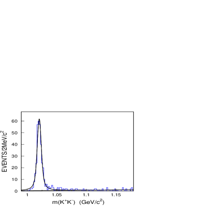
Figure 9: The $m_{K^{+}K^{-}}$ distribution for $J/\psi\rightarrow K^{+}K^{-}\pi^{+}\pi^{-}\pi^{0}$ events. The curves are the results of the fit described in the text.

III.3.2 $J/\psi\rightarrow\phi\eta^{\prime}$

After requiring $0.5<m_{\gamma\gamma}<0.6$ GeV/c² and $m_{\pi^{+}\pi^{-}}<0.45$ GeV/c², the $\pi^{+}\pi^{-}\gamma\gamma$ mass recoiling against the $\phi$($|m_{K^{+}K^{-}}-1.02|<0.02$ GeV/c²), shows a clean $\eta^{\prime}$ peak, as seen in Figure 10. No clear signal is observed for $\phi$ sidebands (0.98 GeV/c${}^{2}<m_{K^{+}K^{-}}<1.0$ GeV/c² and 1.04 GeV/c${}^{2}<m_{K^{+}K^{-}}<1.06$ GeV/c²). The fit of $m_{\pi^{+}\pi^{-}\gamma\gamma}$ yields $198\pm 12$ events with a peak at $959.2\pm 1.4$ MeV/c², and the detection efficiency for this channel is $(7.83\pm 0.14)$%, which gives

$B(J/\psi\rightarrow\phi\eta^{\prime})=(5.11\pm 0.31)\times 10^{-4}.$

Here, the error is statistical only.

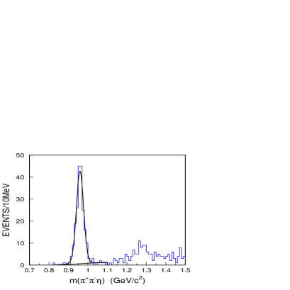
Figure 10: The $m_{\pi^{+}\pi^{-}\gamma\gamma}$ distribution for $J/\psi\rightarrow\phi\pi^{+}\pi^{-}\eta$ candidate events. The curves are the result of the fit described in the text.

III.4 Systematic Errors

In this analysis, the systematic errors on the branching fractions mainly come from the following sources:

III.4.1 MDC tracking efficiency

The MDC tracking efficiency is measured in clean channels like $J/\psi\rightarrow\Lambda\bar{\Lambda}$ and $\psi(2S)\rightarrow\pi^{+}\pi^{-}J/\psi,~{}J/\psi\rightarrow\mu^{+}\mu^{-}$. It is found that the Monte Carlo simulation agrees with data within 1-2% for each charged track. Therefore 4% is taken as the systematic error on the tracking efficiency for the channels with two charged tracks and 8% for the channels with four charged tracks in the final states.

III.4.2 Particle ID

The particle identification (PID) efficiency of the kaon is studied from $J/\psi\rightarrow K^{+}K^{-}\pi^{0}$ and $J/\psi\rightarrow\phi\eta$. The results indicate that the kaon PID efficiency for data agrees well with that of the Monte Carlo simulation in the kaon momentum region less than 1.0 GeV/c. In the analysis of $J/\psi\rightarrow\phi\pi^{0}$, where two charged tracks are required to be kaons, the PID efficiency difference between data and Monte Carlo simulation is about 3.4%. In other decay modes, at least one charged track is required to be identified as a kaon, so the difference from PID is less than 1%. Here, the difference of the PID efficiencies between data and Monte Carlo simulation is taken as one of the systematic errors.

III.4.3 Photon detection efficiency

For the decay modes analyzed in this paper, one or two photons are involved in the final states. The photon detection efficiency is studied from $J/\psi\rightarrow\rho^{0}\pi^{0}$ in Ref. besrhopi . The results indicate that the difference between the detection efficiency of data and MC simulation is less than 2% for each photon.

III.4.4 Kinematic fit

The kinematic fit is a useful tool to improve resolution and reduce background. The systematic error from the kinematic fit is studied with the clean channel $J/\psi\rightarrow\pi^{+}\pi^{-}\pi^{0}$, as described in Ref. besrhopi . The conclusion is that the kinematic fit efficiency difference between data and Monte Carlo simulation is about 4.1%. Using the same method, the decay mode $J/\psi\rightarrow\pi^{+}\pi^{-}\pi^{+}\pi^{-}\pi^{0}$ is also analyzed, and the kinematic fit efficiency difference between data and Monte-Carlo is about 4.3%. In this paper, 5% is conservatively taken to be the systematic error from the kinematic fit for all analyzed decay modes.

III.4.5 Selection criteria

The systematic errors for additional selection criteria in specific decay modes are estimated by comparing the efficiency difference with and without the criterion or replacing it with a very loose requirement. The study indicates that they are not large compared with other systematic errors. The results are listed in Table 1

III.4.6 Uncertainty from hadronic interaction model

Different simulations of the hadronic interaction lead to different efficiencies. In this analysis, two models, FLUKA FLUKA and GCALOR GCALOR , are used in simulating hadronic interactions in the Monte-Carlo. The difference of the detection efficiencies from these two Monte Carlo models is about 3%, which is taken as the systematic error.

III.4.7 Uncertainty of background

The uncertainties of the background in each channel are estimated by changing the background shape in the fit. The results are listed in Table 1.

III.4.8 Intermediate decay branching fractions

The branching fractions of $\phi\rightarrow K^{+}K^{-}$ and the pseudoscalar decays are taken from the PDG. The errors of these branching fractions are systematic errors in our measurements and are listed in Table 1.

The systematic error contributions studied above, the error due to the uncertainty of the number of $J/\psi$ events, and the statistical error of the Monte-Carlo samples are all listed in Table 1. The total systematic error is the sum of them added in quadrature.

Table 1: Summary of systematic errors.

$J/\psi\rightarrow$	$\phi\pi^{0}$	$\phi\eta$			$\phi\eta^{\prime}$
Final states	$K^{+}K^{-}\gamma\gamma$	$K^{+}K^{-}\gamma\gamma$	$K^{+}K^{-}\pi^{+}\pi^{-}\gamma$	$K^{+}K^{-}\pi^{+}\pi^{-}\gamma\gamma$	$K^{+}K^{-}\gamma\gamma$	$K^{+}K^{-}\pi^{+}\pi^{-}\gamma$	$K^{+}K^{-}\pi^{+}\pi^{-}\gamma\gamma$
Error Sources	Relative Error (%)
MDC tracking	4	4	8	8	4	8	8
Particle ID	3.4	$<$1	$<$1	$<$1	$<$1	$<$1	$<$1
Kinematic fit	5	5	5	5	5	5	5
Photon efficiency	4	4	2	4	4	2	4
Selection criteria	2.4	2.4	2.8	1	2.4	2.9	2.2
MC sample	1.2	1.2	1.5	2.1	1.2	1.6	1.8
Hadronic interaction model	3	3	3	3	3	3	3
Background uncertainty	16.7	3.9	1.5	3.4	1.5	2.0	1.5
Intermediate decays	1.2	1.4	2.7	2.2	6.7	3.6	3.6
Total $J/\psi$ events	4.7	4.7	4.7	4.7	4.7	4.7	4.7
Total systematic error	19.7	10.7	12.0	12.6	12.0	12.4	12.7

IV Results and Discussion

The branching fractions of $J/\psi$ decaying into $\phi\pi^{0}$, $\phi\eta$, and $\phi\eta^{\prime}$, measured into different final states, are listed in Table 2. The average value is the weighted mean of the results from the different decay modes, and the PDG value is the world average taken from Ref. pdg2004 . The world averages mainly come from MarkIII and DM2. The results obtained here are not in good agreement with previous measurements. Just as for the branching fraction of $J/\psi\rightarrow\pi^{+}\pi^{-}\pi^{0}$, the branching fraction of $J/\psi\rightarrow\phi\eta$ and $\phi\eta^{\prime}$ are higher than those in the PDG.

In this paper, we measured the branching fractions of $J/\psi$ decays into $\phi$ plus a pseudoscalar. The three branching fractions are not sufficient for a detailed study of pseudoscalar mixing, SU(3) breaking, and the contribution from doubly suppressed OZI processes using the phenomenological model in Ref. theory . However the inconsistency between the results from BESII and those from former measurements emphasize the importance for such a study. After measuring the other decay modes of $J/\psi\rightarrow VP$, such as $J/\psi\rightarrow\omega\pi^{0}$, $\omega\eta$, $\omega\eta^{\prime}$, $\rho\eta$, $\rho\eta^{\prime}$, and $K^{*}K$, it will be important to extract physics with all the relevant measurements again.

Table 2: Branching fractions of $J/\psi\rightarrow\phi\pi^{0}$, $\phi\eta$, and $\phi\eta^{\prime}$.

$J/\psi\rightarrow$	Final states	Branching Fraction ($\times 10^{-4}$)
$\phi\pi^{0}$	$K^{+}K^{-}\gamma\gamma$	$<0.064$ (C.L. 90%) foot
	$K^{+}K^{-}\gamma\gamma$	8.67$\pm$0.19$\pm$0.93
	$K^{+}K^{-}\pi^{+}\pi^{-}\gamma$	9.79$\pm$1.02$\pm$1.17
$\phi\eta$	$K^{+}K^{-}\pi^{+}\pi^{-}\gamma\gamma$	9.41$\pm$0.30$\pm$1.19
	Average	8.99$\pm$0.18$\pm$0.89
	PDG	$6.5\pm 0.7$
	$K^{+}K^{-}\gamma\gamma$	6.10$\pm$1.34$\pm$0.73
$\phi\eta^{\prime}$	$K^{+}K^{-}\pi^{+}\pi^{-}\gamma$	5.64$\pm$0.35$\pm$0.70
	$K^{+}K^{-}\pi^{+}\pi^{-}\gamma\gamma$	5.11$\pm$0.31$\pm$0.65
	Average	5.40$\pm$0.25$\pm$0.56
	PDG	$3.3\pm 0.4$

References

(1) H. E. Haber, J. Perrier, Phys. Rev. D 32, 2961 (1985).
(2) R. M. Baltrusaitis et al., Phys. Rev. D 32, 2883 (1985).
(3) D. Coffman et al., Phys. Rev. D 38, 22695 (1988).
(4)J. Jousset et al., Phys. Rev. D 41, 1389 (1990).
(5) J. Z. Bai et al., Nucl. Instrum. Methods
A 458, 627 (2001).
(6) J. Z. Bai et al., Phys. Rev. D 70, 012005 (2004).
(7) S. Eidelman et al. (Particle Data
Group), Phys. Lett. B 592, 1 (2004), and references therein.
(8)
J. J. Aubert et al., Phys. Rev. Lett. 33, 1404 (1974);
J. E. Augustin et al., Phys. Rev. Lett. 33, 1406 (1974);
B. Jean-Marie et al., Phys. Rev. Lett. 36, 291 (1976);
W. Braunschweig et al., Phys. Lett. 63B, 487 (1976);
W. Bartel et al., Phys. Lett. 64B, 483 (1976);
PLUTO collaboration, Phys. Lett. 72B, 493 (1978);
DASP collaboration, Phys. Lett. 74B, 292 (1978);
D. Coffman et al., Phys. Rev. D 38, 2695 (1988);
J. Z. Bai et al., Phys. Rev. D 54, 1221 (1996).
(9) The angular distribution is described by
where is the angle between the vector meson and the positron
direction. and describe the decay products of the vector
meson in its helicity frame.
For , and are the polar
and azimuthal angles of the
momentum of with respect to the helicity direction of the .
(10) S. S. Fang et al.,
High Energy Phys. Nucl. Phys. 27, 277 (2003) (in Chinese).
(11) K. Hanssgen, H.-J.Mohring and J. Ranft, Nucl. Sci. Eng.
88, 551 (1984);
J. Ranft and S. Ritter, Z. Phys. C 20, 347 (1983);
A. Fasso et al., FLUKA 92, Proceedings of the Workshop on Simulating
Accelerator Radiation Environments, Santa Fe, 1993.
(12)C. Zeitnitz and
T. A. Gabriel, Nucl. Instrum. Methods A 349, 106 (1994).
(13) To conservatively estimate the upper limit, the result
obtained from
formula in Section. III is corrected by dividing a factor . Here,
is the systematic error for this decay mode.