EUROPEAN LABORATORY FOR PARTICLE PHYSICS

CERN-PH-EP-2004-032

CERN-AB-2004-030 OP

27 July 2004

Calibration of centre-of-mass energies at LEP 2
for a precise measurement of the W boson mass

The LEP Energy Working Group

R. Assmann¹, E. Barbero Soto¹, D. Cornuet¹, B. Dehning¹, M. Hildreth^1a, J. Matheson^1b, G. Mugnai¹, A. Müller^1c, E. Peschardt¹, M. Placidi¹, J. Prochnow¹, F. Roncarolo^1,2, P. Renton³, E. Torrence^1,4d, P. S. Wells¹, J. Wenninger¹, G. Wilkinson³

¹CERN, European Organisation for Particle Physics, CH-1211 Geneva 23, Switzerland
²University of Lausanne, CH-1015 Lausanne, Switzerland
³Department of Physics, University of Oxford, Keble Road, Oxford OX1 3RH, UK
⁴Enrico Fermi Institute and Department of Physics, University of Chicago, Chicago IL 60637, USA
^aNow at: University of Notre Dame, Notre Dame, Indiana 47405, USA
^bNow at: CCLRC Rutherford Appleton Laboratory, Chilton, Didcot, Oxfordshire, OX11 OQX, UK
^cNow at: ISS, Forschungszentrum Karlsruhe, Karlsruhe, Germany
^dNow at: University of Oregon, Department of Physics, Eugene OR 97403, USA

The determination of the centre-of-mass energies for all LEP 2 running is presented. Accurate knowledge of these energies is of primary importance to set the absolute energy scale for the measurement of the W boson mass. The beam energy between 80 and 104 GeV is derived from continuous measurements of the magnetic bending field by 16 NMR probes situated in a number of the LEP dipoles. The relationship between the fields measured by the probes and the beam energy is defined in the NMR model, which is calibrated against precise measurements of the average beam energy between 41 and 61 GeV made using the resonant depolarisation technique. The validity of the NMR model is verified by three independent methods: the flux-loop, which is sensitive to the bending field of all the dipoles of LEP; the spectrometer, which determines the energy through measurements of the deflection of the beam in a magnet of known integrated field; and an analysis of the variation of the synchrotron tune with the total RF voltage. To obtain the centre-of-mass energies, corrections are then applied to account for sources of bending field external to the dipoles, and variations in the local beam energy at each interaction point. The relative error on the centre-of-mass energy determination for the majority of LEP 2 running is $1.2\times 10^{-4}$, which is sufficiently precise so as not to introduce a dominant uncertainty on the W mass measurement.

To be submitted to Eur. Phys. J. C.

1 Introduction

The operation of the large electron-positron (LEP) collider in the years 1996 to 2000 (LEP 2) saw the delivery of almost 700 ${\mathrm{pb^{-1}}}$ of integrated luminosity to each experiment at $\mathrm{e}^{+}\mathrm{e}^{-}$ collision energies above the W-pair production threshold. A primary physics motivation for the LEP 2 programme was the precision measurement of the W boson mass, $M_{\mathrm{W}}\,\approx\,80.4~{}\mathrm{GeV}/c^{\mathrm{2}}$. The centre-of-mass energy, $E_{\mathrm{CM}}$, establishes the absolute energy scale for this measurement, and any uncertainty in this quantity leads to an uncertainty of $\Delta M_{\mathrm{W}}/M_{\mathrm{W}}\approx\Delta E_{\mathrm{CM}}/E_{\mathrm{CM}}$. The statistical precision on the full LEP 2 data set is around 30 MeV [1]. To avoid a significant contribution to the total error, this sets a target of $\Delta E_{\mathrm{CM}}/E_{\mathrm{CM}}\,=\,1-2\times 10^{-4}$. This paper reports on the determination of the centre-of-mass energies for all LEP 2 operation. The results supersede those in an earlier publication concerning the 1996 and 1997 LEP runs [2].

In the following section the main concepts which will be used in the subsequent analysis are introduced, together with a brief year-by-year description of LEP 2 operation. The method of the energy determination is then presented.

The starting point of the energy determination is a set of precise calibrations of the mean beam energy around the ring, $E_{\mathrm{b}}$, performed with the resonant depolarisation (RDP) technique at energies of $41<E_{\mathrm{b}}<61~{}\mathrm{GeV}$. The NMR magnetic model relates these calibrations to field measurements made by NMR probes in selected dipoles. The model is then used to set the absolute energy scale for physics running in the regime $81<E_{\mathrm{b}}<104~{}\mathrm{GeV}$. RDP and the calibration of the magnetic model are explained in section 3. Corrections are applied to this energy estimate to account for variations with time in the dipole strength during data-taking, and additional sources of bending field, such as those arising from non-central orbits in the quadrupoles. These corrections are described in section 4. The NMR estimate together with these corrections forms the full $E_{\mathrm{b}}$ model.

In calculating the centre-of-mass energy at each experimental interaction point it is necessary to know the local beam energy, which differs significantly from $E_{\mathrm{b}}$ around the ring due to losses from synchrotron radiation and the boosts provided by the RF system. Other potential corrections to $E_{\mathrm{CM}}$ come from the correlated effects of dispersion and collision offsets, and any difference in energy between the electron and positron beams. These issues are discussed in section 5.

The most important uncertainty in the energy determination is that associated with the NMR magnetic model. This error is assigned from the results of three complementary approaches, which in different manners attempt to quantify the agreement between the model and the true energy in the physics regime.

1. The flux-loop was a sequence of copper loops which were embedded in the dipole cores and connected in series and which sensed the change of flux as the magnets were ramped. The number of NMR-equipped dipoles used in the magnetic model was limited, but comparison with the flux-loop data allows the representability of this sampling to be assessed. Flux-loop data were accumulated in dedicated measurements throughout LEP 2 operation which can be used to constrain the model, as is explained in section 6.

2. The spectrometer was a device installed and commissioned in 1999 and used throughout the 2000 run. It consisted of a steel dipole with precisely known integrated field, and triplets of beam-position monitors (BPMs) on either side which enabled the beam deflection to be measured, and thus the energy to be determined. The spectrometer apparatus and calibration is outlined in section 7, and the data analysis is presented in section 8.

3. In a machine such as LEP the synchrotron tune, $Q_{s}$, depends on the beam energy, the energy loss per turn, and the total RF voltage, $V_{\mathrm{RF}}$. Since the energy loss itself depends on the beam energy, an analysis of the variation of $Q_{s}$ with $V_{\mathrm{RF}}$ can be used to infer $E_{\mathrm{b}}$. Experiments were conducted in 1998, 1999 and 2000 to exploit this method. A full description is given in section 9.

The results of the three approaches can be assessed for compatibility. If consistent, they may be combined to set both a correction and an associated uncertainty for the magnetic model. Such an analysis is presented in section 10. The resulting uncertainty, together with the uncertainties from other sources, is used in section 11 to assign the total error on the collision energies.

The spread in the collision energies is relevant in the analysis of the W boson width. The understanding of the energy spread is described in section 12. The conclusions of the energy analysis can be found in section 13.

2 The LEP Machine and the LEP 2 Programme

2.1 LEP Beam Energy and Synchroton Energy Loss

The energy, $E_{\mathrm{b}}$, of a beam of ultra-relativistic electrons or positrons in a closed orbit is directly proportional to the bending field, $B$, integrated around the beam trajectory, $s$:

$$E_{\mathrm{b}}\ =\frac{ec}{2\pi}\oint B\,\mathrm{ds}.$$ (1)

For LEP 98% of the nominal bending field was provided by 3280 concrete-reinforced dipole magnets, of approximate length 5.8 m and field of 1070 G at $E_{\mathrm{b}}=100~{}\mathrm{GeV}$. The remaining 2% was dominated by steel-cored dipoles in the injection region, with a small contribution coming from the special weak dipoles designed to match the arcs to the straight sections. There were other possible sources of effective dipole field, such as the quadrupole magnets on the occasions when the mean beam trajectory was not centred. Expression 1 is assumed in constructing the NMR magnetic model and is fundamental to the LEP 2 energy calibration.

As the beams circulate they lose energy through synchrotron radiation. The energy loss per turn, $U_{0}$, is given by:

$$U_{0}=\frac{C_{\gamma}\,(ec)^{2}}{2\pi}\oint E_{\mathrm{b}}^{2}B^{2}\mathrm{ds},$$ (2)

where the constant $C_{\gamma}\equiv e^{2}/3\epsilon_{0}(m_{e}c^{2})^{3}=8.86\times 10^{-5}\,\mathrm{(GeV)^{-3}}$. This relation, together with expression 1 gives:

$$U_{0}=C_{\gamma}\frac{E_{\mathrm{b}}^{4}}{\rho}.$$ (3)

Here $\rho$ is the effective bending radius, which in the case of LEP was approximately 3026 m. Expression 3 gives an energy loss per turn of 2.9 GeV at beam energies of 100 GeV.

The synchrotron energy loss is replenished by the RF system. In the LEP 2 era this consisted of stations of super-conducting cavities situated on either side of the four experimental interaction points. The installation of new cavities, and increases to the field gradient of the existing klystrons, enabled the voltage of the RF system to be augmented each year of LEP 2 operation. Understanding the variation in beam energy around the ring from synchrotron losses and RF boosts is an important ingredient in the energy model. Furthermore, the measurement of quantities sensitive to the energy loss, such as the synchrotron tune, can be used to determine the beam energy itself.

2.2 LEP 2 Datasets and Operation

The LEP 2 programme began in 1996 when the collision energy of the beams was first ramped to the $W^{+}W^{-}$ production threshold of 161 GeV, and approximately $10~{}\mathrm{pb^{-1}}$ of integrated luminosity was collected by each experiment. Later in that year LEP was run at 172 GeV, and a dataset of similar size was accumulated. In each of the four subsequent years of operation the collision energy was raised to successively higher values, such that almost half the integrated luminosity was delivered at nominal collision energies of 200 GeV and above. The motivation for this policy was to improve the sensitivity in the search for the Higgs boson and other new particles. The step-by-step nature of the energy increase was dictated by the evolving capabilities of the RF system. The nominal energy points of operation, $E_{\mathrm{CM}}^{\mathrm{nom}}$, are listed in table 1, together with the approximate integrated luminosities delivered to each experiment.

Year	1996		1997	1998	1999				2000
$E_{\mathrm{CM}}^{\mathrm{nom}}$  [GeV]	161	172	183	189	192	196	200	202	205	207
$\int{\cal{L}}\,dt$ [$\mathrm{pb^{-1}}$]	10	10	54	158	26	76	83	41	83	140
Physics optics	90/60		90/60	102/90	102/90				102/90
	(108/90)		(102/90)
Polarisation optics	90/60		60/60	60/60	60/60				101/45
					(101/45)

Table 1: Summary of the LEP 2 running parameters and performance. Shown for each year are the nominal collision energies; the integrated luminosities collected by a typical experiment; the choice of optics for the majority of the physics running (‘physics optics’) and the preferred optics used for RDP calibration (‘polarisation optics’). (Alternative choices of optics used during the run are given in parentheses.) The values given for the optics signify the betatron phase advance in degrees between the focusing quadrupoles in the horizontal/vertical planes.

During normal operation the machine would be filled with four electron and four positron bunches at $E_{\mathrm{b}}\approx 22~{}\mathrm{GeV}$, and the beams would then be ramped to physics energy, at which point they would be steered into collision and experimental data-taking began. The fill would last until the beam currents fell below a useful level, or an RF cavity trip precipitated the loss of the beam. The mean fill lengths ranged from 5 hours in 1996 to 2 hours in 1999. After de-gaussing the magnets the cycle would be repeated. Following the experience gained at LEP 1 [3], bending modulations were performed in the 1997–1999 runs prior to colliding the beams, in which the dipole current was modulated with a sequence of very small square pulses. The purpose of this exercise was to condition the magnets and suppress the effects of parasitic currents.

In 2000, the operation was modified in order to optimise still further the high-energy reach of LEP [4]. Fills were started at a beam energy safely within the capabilities of the RF system. When the beam currents had decayed significantly, typically after an hour, the dipoles were ramped and luminosity was delivered at a higher energy. This procedure was repeated until the energy was at the limit of the RF, and data taken until the beam was lost through a klystron trip. These miniramps lasted less than a minute, and varied in step size with a mean value of 600 MeV. Hardware signals were used to flag the start and end of miniramps to the experiments, which continued to take data throughout, and this information was recorded with the logged triggers. The starting energy of fills, and the precise strategy of miniramping varied throughout the year, depending on the status of the RF system. The luminosity in 2000 was therefore delivered through a near-continuum of energies. The sub-fills on either side of the miniramps can be seen in the ‘fine structure’ of figure 1 (a) and 1 (b), which display the distribution of luminosity both with $E_{\mathrm{CM}}$ and time for a single experiment. The coarser bands in the plots arise through the choice of starting energy for the fill, a decision dependent on the status of the RF system. The two $E_{\mathrm{CM}}^{\mathrm{nom}}$ points listed in table 1 refer to the integrated totals delivered below and above an arbitrary division value of 205.5 GeV. The lower of these two bins is dominated by data accumulated in the earlier part of the run.

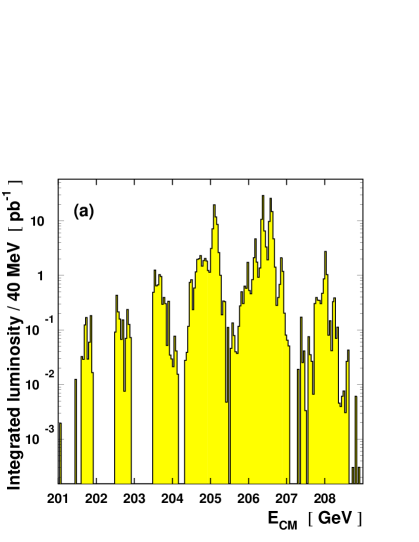
Figure 1: Distributions of collected luminosity for a single LEP experiment in 2000. (a) shows the integrated luminosity in bins of $E_{\mathrm{CM}}$. (b) shows the variation of $E_{\mathrm{CM}}$ against day of year; each entry corresponds to the mean energy for a data file of maximum length $\sim 30$ minutes. The values of $E_{\mathrm{CM}}$ have been calculated using the full energy model.

Another aspect of operation which was unique to 2000, also deployed to optimise the collision energy within the restrictions of the available RF voltage, was the coherent powering of corrector magnets to apply a so-called bending-field spreading (BFS) boost. The BFS is discussed in section 4.3.

In addition to the high-energy running summarised in table 1, each year a number of fills were performed at the ${\mathrm{Z}}$ resonance. This was to provide calibration data for the experiments. During 1997, some data were also collected at nominal centre-of-mass energies of 130-136 GeV, to investigate effects seen during operation at similar energies in 1995. Finally, several fills were devoted to energy-calibration activities, most notably RDP, spectrometer and $Q_{s}$ measurements. Most of these energy-calibration experiments were conducted with single beams, and many of them spanned a variety of energy points.

Included in the information of table 1 are the machine optics which were used for physics operation (‘physics optics’) and for RDP measurements (‘polarisation optics’). The values signify the betatron phase advance in degrees between the focusing quadrupoles of the LEP arcs in the horizontal/vertical planes. The choice of optics evolved throughout the programme in order to optimise the luminosity at each energy point. Certain optics enhanced the build-up of polarisation, and thus were favoured for RDP measurements. As is explained in section 4, the optics influences $E_{\mathrm{b}}$ in several ways, which must be accounted for in the energy model.

3 RDP and the NMR Magnetic Model

The LEP 2 energy scale is set by the NMR magnetic model. Between beam energies of 41 and 61 GeV precise measurements of $E_{\mathrm{b}}$ are provided by resonant depolarisation (RDP). Also available are local measurements of the bending field, made by NMR probes in selected dipoles. Following expression 1, and taking the probes to be representative of the total bending field, the magnetic model is calibrated through a linear fit between the RDP measurements and the NMR readings at low energy. Applying this calibrated model at high-energy fixes $E_{\mathrm{b}}^{\mathrm{NMR}}$, the dipole contribution to the beam energy in physics operation. Onto $E_{\mathrm{b}}^{\mathrm{NMR}}$ must be added corrections coming from sources of bending field external to the dipoles.

Possible sources of error in the NMR model arise from the limited sampling of the total bending field provided by the probes, and the consequences of any non-linearity in the relationship between the field and $E_{\mathrm{b}}$, when extrapolated up to high energy.

3.1 RDP Measurements

The best determination of the beam energy at a particular time is by means of RDP. The beam can build up a non-negligible transverse polarisation through the Sokolov-Ternov mechanism [5]. The degree of polarisation can be measured by the angular distribution of Compton-scattered polarised laser light. By exciting the beam with a transverse oscillating magnetic field, this polarisation can be destroyed when the excitation frequency matches the spin precession frequency. Determining the RDP frequency allows a precise determination of $E_{\mathrm{b}}$ through:

$$E_{\mathrm{b}}\ =E_{\mathrm{b}}^{\mathrm{RDP}}\ \equiv\frac{\nu_{s}\,.\,m_{e}\,c^{2}}{(g_{e}\,-\,2)/2},$$ (4)

where $\nu_{s}$ is the ‘spin-tune’, that is the number of electron-spin precessions per turn, $m_{e}$ is the electron mass and $(g_{e}-2)/2$ is the magnetic-moment anomaly of the electron. The beam energy measured by RDP is the average around the ring and over all particles. The intrinsic precision of RDP at the Z resonance is estimated to be 200 keV [6].

At LEP 2 physics energies RDP cannot be performed. The relative spread of the beam energy grows linearly with $E_{\mathrm{b}}$ and consequently it becomes increasingly probable that the beam will encounter machine imperfections which inhibit the build-up of polarisation. RDP measurements made at low energies are instead used to calibrate the NMR model, which is then applied in the physics regime. The systematic uncertainties in this procedure can be minimised by making the span of RDP measurements as wide as possible, in particular at high energy. Therefore during the LEP 2 programme techniques were developed to reduce the machine imperfections and enhance the polarisation levels during RDP calibration. These included the ‘k-modulation’ studies to measure the offsets between beam pick-ups and quadrupole centres [7], the improved use of magnet-position surveys, and the development of dedicated polarisation optics [8]. The maximum energy at which sufficient polarisation was obtained for a reliable calibration measurement was 61 GeV. The time required for a complete measurement at each energy point was several hours.

Fill	Date	41 GeV	45 GeV	50 GeV	55 GeV	61 GeV	Optics
3599	19 Aug ’96			$\bullet$			90/60
3702	31 Oct ’96		$\bullet$				90/60
3719	3 Nov ’96		$\bullet$	$\bullet$			90/60
4000	17 Aug ’97		$\bullet$				90/60
4121	6 Sept ’97		$\bullet$	$\bullet$			60/60
4237	30 Sept ’97		$\bullet$	$\bullet$			60/60
4242	2 Oct ’97	$\bullet$	$\bullet$	$\bullet$	$\bullet$		60/60
4274	10 Oct ’97		$\bullet$				90/60
4279	11 Oct ’97	$\bullet$	$\bullet$	$\bullet$	$\bullet$		60/60
4372	29 Oct ’97	$\bullet$	$\bullet$				60/60
4666	14 June ’98		$\bullet$	$\bullet$	$\bullet$		60/60
4669	18 June ’98		$\bullet$				102/90
4843	15 July ’98		$\bullet$		$\bullet$		60/60
5137	6 Sept ’98		$\bullet$				60/60
5141	7 Sept ’98	$\bullet$	$\bullet$	$\bullet$			60/60
5214	20 Sept ’98	$\bullet$	$\bullet$	$\bullet$	$\bullet$	$\bullet$	60/60
5232	29 Sept ’98		$\bullet$				102/90
5337	18 Oct ’98	$\bullet$	$\bullet$	$\bullet$	$\bullet$	$\bullet$	60/60
5670	7 June ’99	$\bullet$	$\bullet$				60/60
5799	25 June ’99	$\bullet$	$\bullet$	$\bullet$			60/60
5969	22 July ’99	$\bullet$					60/60
5971	22 July ’99		$\bullet$	$\bullet$			60/60
6087	8 Aug ’99				$\bullet$		60/60
6302	9 Sept ’99	$\bullet$	$\bullet$	$\bullet$	$\bullet$		60/60
6371	20 Sept ’99	$\bullet$	$\bullet$	$\bullet$	$\bullet$		60/60
6397	25 Sept ’99		$\bullet$	$\bullet$			101/45
6404	26 Sept ’99	$\bullet$	$\bullet$	$\bullet$	$\bullet$		60/60
6432	29 Sept ’99		$\bullet$	$\bullet$			101/45
6509	9 Oct ’99	$\bullet$		$\bullet$		$\bullet$	101/45
6627	27 Oct ’99		$\bullet$				102/90
7129	11 May ’00	$\bullet$	$\bullet$	$\bullet$			101/45
7251	25 May ’00	$\bullet$	$\bullet$	$\bullet$			101/45
7519	21 June ’00	$\bullet$		$\bullet$			101/45
7929	26 July ’00	$\bullet$					101/45
8368	4 Sept ’00	$\bullet$		$\bullet$	$\bullet$		101/45
8446	11 Sept ’00	$\bullet$					101/45
8556	25 Sept ’00		$\bullet$	$\bullet$	$\bullet$		101/45

Table 2: Successful RDP measurements at LEP 2. Measured energy points are marked $\bullet$.

The full list of LEP 2 RDP measurements is shown in table 2, indicating the fill number, date, nominal values of $E_{\mathrm{b}}$ calibrated and optics used. In total 86 energy points, distributed through 37 fills, were calibrated. The lowest energy measured was 41 GeV, a value dictated by the range of sensitivity of the NMR probes. Care was taken to perform a subset of the measurements with physics optics as well, to allow for a cross-check against optics dependent effects not foreseen in the the energy model.

3.2 The NMR Probes and the NMR Magnetic Model

The NMR probes measured the local magnetic field with a relative precision of $10^{-6}$. Throughout LEP 2 operation a total of 16 probes were read out during physics and RDP operation. Time-integrated readings were logged every 5 minutes. During the 2000 run additional records were logged in response to rapid changes in field during miniramps. In the analysis the probes are designated by their octant location. Each LEP octant had at least one probe, while octants 1 and 5 each had strings of five probes (1a–e; 5a–e). Probes 1c and 1d were situated in the same dipole. Other dipoles in the injection region, and the spectrometer, were also instrumented with probes for limited periods of the programme, but these are not included in the NMR model.

The NMR probes were located underneath the vacuum chamber above a steel field plate, installed to improve the uniformity of the local field. Radiation damage from synchrotron light led to a reduction in the probe locking efficiency, particularly at low energy. In response to this problem the probes were replaced, typically two to three times a year. Precision mounts first used in 1997 ensured that the replacement probes were installed to within 0.5 mm of their nominal positions.

In the NMR model the magnetic fields $B^{\mathrm{NMR}\,i}$ measured by each NMR $i=~{}\mathrm{1a},..,8$, after ramping to the excitation current of interest, are converted into an equivalent raw beam energy $E_{\mathrm{b}}^{\mathrm{NMR}\,i}$. The relation is assumed to be linear, of the form

$$E_{\mathrm{b}}^{\mathrm{NMR}\,i}=a^{i}\,+\,b^{i}B^{\mathrm{NMR}\,i},$$ (5)

with $E_{\mathrm{b}}^{\mathrm{NMR}}$ being used to signify the average over all $E_{\mathrm{b}}^{\mathrm{NMR}\,i}$.

Because the NMR probes are only sensitive to the dipole fields, it is necessary to account for the other sources of bending field in order to have the best possible model of the beam energy. Therefore $E_{\mathrm{b}}^{\mathrm{NMR}\,i}$ is corrected to

$$E_{\mathrm{b}}^{\mathrm{MOD}\,i}=E_{\mathrm{b}}^{\mathrm{NMR}\,i}\,+\,\sum\Delta E_{\mathrm{b}},$$ (6)

where the sum runs over all the additional components in the energy model detailed in section 4. These corrections are common to all NMRs and include energy changes between the end of ramp and the time of interest. In the calibration procedure the two parameters $a^{i}$ and $b^{i}$ for each probe are determined by a fit to the energies measured by RDP. Thereafter, all available values of $E_{\mathrm{b}}^{\mathrm{MOD}\,i}$ are averaged together to give $E_{\mathrm{b}}^{\mathrm{MOD}}$, which is taken as the energy model’s estimate of $E_{\mathrm{b}}$. At LEP 2 energies the error associated with $E_{\mathrm{b}}^{\mathrm{MOD}}$ arising from the uncertainty in the RDP measurements themselves is less than 0.5 MeV.

3.3 NMR Residuals, High-Energy Scatter and Stability with Time

The NMR model has been calibrated against the RDP data of each year separately, and the results of these fits are used to define the energy model for that year. As the calibration coefficients are observed to be very stable for 1997 onwards, a calibration has also been made against the complete 1997–2000 dataset. (This global fit can not be extended to 1996 because of differences in the exact probe locations for this year.) The mean (and RMS) coefficients averaged over the 16 probes are found to be $\langle a\rangle=91.17(0.24)$ MeV/Gauss and $\langle b\rangle=22(61)$ MeV. No significant difference is found between the fit results for different optics.

Figure 2 shows the residuals of the separate fits to the RDP data, averaged over the probes, for the main datasets and those of the global fit. The error bars are the statistical uncertainties on the mean of all the contributing measurements. There is a small, but characteristic, non-linearity over the sampled energy range.

Figure 2: Residuals of the fitted energy model to the RDP data in 1997-2000. Each point is the mean over the available measurements at that energy, with the error bar the statistical uncertainty on this mean. The horizontal positions of the points have been slightly adjusted to aid clarity.

The residuals of the individual NMRs entering in figure 2 agree to within a few MeV. When the model is applied at high energy, however, the individual non-linearities of each magnet, and the lever-arm over which the calibration is extrapolated, lead to a significant scatter in the prediction of $E_{\mathrm{b}}^{\mathrm{NMR}}$. Figure 3 shows the relative differences between $E_{\mathrm{b}}^{\mathrm{NMR}\,i}$ and $E_{\mathrm{b}}^{\mathrm{NMR}}$ evaluated during high-energy physics operation, averaged over all 1997–2000 data. The error bars are half the difference between the maximum and minimum values in these years. There is no strong evidence of systematic structure in this distribution, although the differences for those probes in octant 1 are predominantly positive in sign, and those in octant 5 are predominantly negative. The RMS of the individual probe predictions is $43\times 10^{-5}$. If the measurements of the 16 probes are representative of the 3280 dipoles in LEP, then the expected precision of the dipole part of the model at $E_{\mathrm{b}}=100\,\mathrm{GeV}$ is 11 MeV. The purpose of the flux-loop, spectrometer and $Q_{s}$ measurements presented in the following sections is to test this assumption and to constrain further any offset between the model prediction and the true energy.

Figure 3: Relative differences between the individual probe predictions of the dipole energy and that of the average, evaluated at physics energy and averaged over 1997–2000. The error bars are half the difference between the maximum and minimum values in these years.

Both figures 2 and 3 illustrate the stability of the NMR calibration with time. This can be seen in a more quantitative fashion by using the calibration coefficients of one year to evaluate $E_{\mathrm{b}}^{\mathrm{NMR}}$ during physics operation in another year. The luminosity-weighted mean shifts in results are presented in table 3, and are always 4 MeV or less. Larger shifts of around 30 MeV are seen when a later year’s calibration coefficients are applied to the 1996 data, a difference attributable to the change in probe locations after the 1996 run.

	Dataset
Fit	’97	’98	’99	’00
’97	/	4.1	1.5	0.9
’98	-3.6	/	-2.5	-0.3
’99	-1.8	1.9	/	2.1
’00	-3.6	-0.1	-1.7	/
’97-’00	-2.0	1.8	-0.6	1.8

Table 3: Shift in $E_{\mathrm{b}}^{\mathrm{NMR}}$ (MeV) observed in physics operation when the data are reprocessed with NMR calibration coefficients determined by a fit to the RDP data of another year.

4 Other Components of the $E_{\mathrm{b}}$ Model

The NMR fit gives the value of the energy from the dipole magnets at start-of-fill. The complete $E_{\mathrm{b}}$ model adds to this contributions coming from variations of the dipole magnet strength during the fill, as well as additional sources of bending field arising from quadrupole effects, horizontal correctors, and uncompensated currents flowing in the magnet power bars. These additional model components, represented by $\sum\Delta E_{\mathrm{b}}$ in expression 6, are discussed in this section. The relative importance of the model components during physics running can be assessed from table 4, which shows the luminosity-weighted contribution of each term to $E_{\mathrm{b}}^{\mathrm{MOD}}$ at each high-energy point of the LEP 2 programme.

Year	’96		’97	’98	’99				’00
$E_{\mathrm{CM}}^{\mathrm{nom}}$  [GeV]	161	172	183	189	192	196	200	202	205	207
$\mathrm{f_{c}^{RF}}$	-13.8	-14.2	-20.2	-27.5	1.2	-27.8	-40.0	-24.4	-32.3	-40.2
$\mathrm{f^{RF}}$	0.0	-3.0	-152.4	-187.0	-222.2	-229.7	-194.9	-129.8	-85.9	-29.6
NMR rise	3.6	7.0	1.7	0.8	0.7	-0.1	-0.7	-0.7	1.5	2.2
Tides	1.1	0.8	1.2	1.7	1.9	2.2	1.4	1.8	2.0	1.8
Hcor / BFS	-2.8	-3.0	-5.6	-7.8	-1.1	-1.6	-0.4	1.1	357.6	430.0
QFQD	-2.6	-2.4	-2.8	-1.3	-1.3	-1.4	-1.4	-1.4	-1.4	-1.4

Table 4: The luminosity-weighted corrections to $E_{\mathrm{b}}^{\mathrm{MOD}}$ in MeV from each component in the energy model at each nominal energy point.

4.1 Quadrupole Effects

In a very high-energy synchrotron, such as LEP, the orbit length is fixed by the RF frequency, $\mathrm{f^{RF}}$. The central RF frequency, $\mathrm{f_{c}^{RF}}$corresponds to that orbit where the beam passes on average through the centre of the quadrupoles. When the RF frequency $\mathrm{f^{RF}}$ does not coincide with $\mathrm{f_{c}^{RF}}$, the beam senses on average a dipole field in the quadrupoles, which causes a change in the beam energy, $\Delta E_{\mathrm{b}}$, of:

$$\frac{\Delta E_{\mathrm{b}}}{E_{\mathrm{b}}}\>=\>-\frac{1}{\alpha_{c}}\,\frac{\mathrm{f^{RF}}\,-\,\mathrm{f_{c}^{RF}}}{\mathrm{f^{RF}}},$$ (7)

where $\alpha_{c}$ is the momentum compaction factor, the optics dependent values of which are listed in table 5, as calculated by the simulation program MAD [24]. The nominal value of $\mathrm{f_{c}^{RF}}$ is 352,254,170 Hz. The consequences of variations in both $\mathrm{f^{RF}}$ and $\mathrm{f_{c}^{RF}}$ must be corrected for in the energy model.

Optics		$\alpha_{c}$ [ $\times 10^{-4}$ ]
	90/60	1.86
Physics	108/90	1.43
	102/90	1.56
	60/60 (1997-98)	3.87
Polarisation	60/60 (1999)	3.77
	101/45	1.50

Table 5: Calculated values of the momentum compaction factor, $\alpha_{c}$, for the physics and polarisation optics of the LEP 2 programme. The estimated relative uncertainties are 1%.

4.1.1 Central Frequency and Machine Circumference: $\Delta E_{\mathrm{b}}\,(\mathrm{f^{RF}_{c}})$

The central frequency was measured only on a few occasions during a year’s running and required non-colliding beams [9]. In between these measurements, $\mathrm{f_{c}^{RF}}$ can be interpolated through $x_{\mathrm{arc}}$, the average horizontal beam position in the LEP arcs as measured by the beam-position monitors (BPMs) at a defined RF frequency [10]. These measurements are shown in figure 4 for 1997-2000, where the $x_{\mathrm{arc}}$ data have been normalised to the actual $\mathrm{f_{c}^{RF}}$ measurements. The central frequency can be seen to change by 20–30 Hz, and evolves in a similar fashion over the course of each year. The evolution indicates a change in the machine circumference, one which is believed to be driven by a seasonal variation in the pressure of the water-table and the level of Lac Léman.

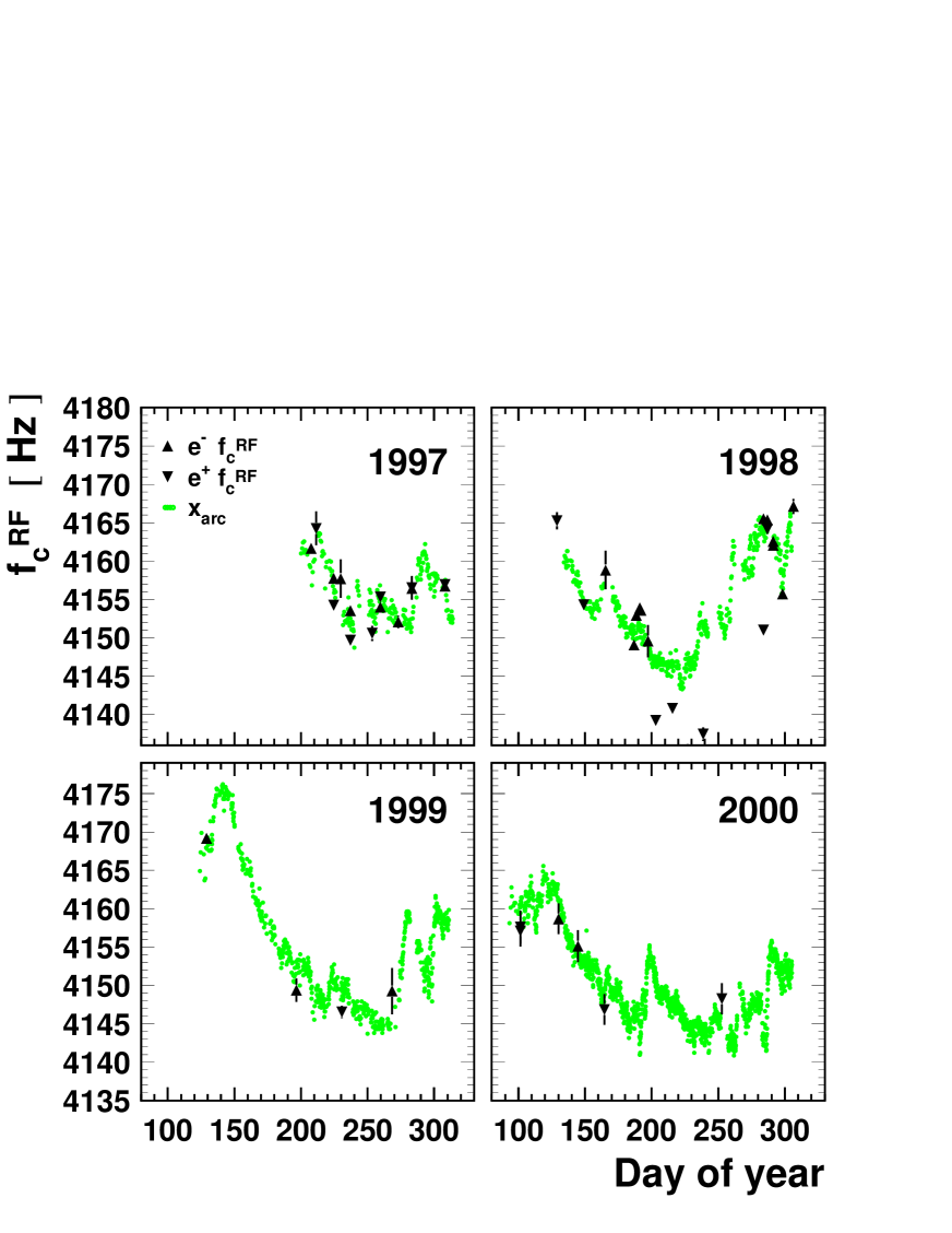
Figure 4: Evolution of the central frequency as a function of time for the four main datasets of the LEP 2 programme. Shown are both the actual $\mathrm{f_{c}^{RF}}$measurements, and the values extracted from $x_{\mathrm{arc}}$, after correction for tides. Note that the vertical scale shows a variation in the last four digits of the LEP RF frequency, which is nominally $352\,254\,170$ Hz.

The $\mathrm{f_{c}^{RF}}$ and $x_{\mathrm{arc}}$ measurements together allow the energy to be corrected fill by fill. The average values of this correction are listed in table 4 and are found to be similar year to year. The variation seen within 1999 comes about because the running at each energy point was concentrated at different periods of the year, rather than uniformly distributed.

The uncertainty on this correction is set by studying the agreement between the direct $\mathrm{f_{c}^{RF}}$ measurements and $x_{\mathrm{arc}}$. In general these are consistent, although there are occasional discrepancies, such as for some of the $\mathrm{e}^{+}$ data in 1998. Globally the agreement is found to be good to $\pm 2\,\mathrm{Hz}$. Any bias in $\mathrm{f_{c}^{RF}}$ will apply to both the low-energy calibration data and the high-energy running. As the correction scales with energy, the effect of a bias will be absorbed in the calibration coefficients and lead to no net error at high energy. This argument is only valid, however, when the optics, and therefore $\alpha_{c}$, is the same for calibration and physics operation. This was the case in 1996, and approximately so in 2000, but not in the other years, where the uncertainty in $\mathrm{f_{c}^{RF}}$ induces a residual $3\times 10^{-5}$ error on $E_{\mathrm{b}}^{\mathrm{MOD}}$.

The LEP circumference was also distorted by the gravitational mechanism of earth tides, as discussed in section 4.2.2. These effects have been subtracted in the $\mathrm{f_{c}^{RF}}$ analysis. The $\mathrm{f_{c}^{RF}}$ and $x_{\mathrm{arc}}$ measurements used in this analysis have also been corrected for residual biases from horizontal corrector effects [9], discussed in section 4.3.

4.1.2 RF Frequency Shifts: $\Delta E_{\mathrm{b}}\,(\mathrm{f^{RF}})$

For 1997 and subsequent years the RF frequency was routinely increased by $\sim 100$ Hz from the nominal value in order to change the horizontal damping partition number. This was done to squeeze the beam more in the horizontal plane, which benefited both the specific luminosity and the machine background at the experiments. A side-effect of this strategy was that the beam energy was reduced, following equation 7. Since the 2000 run placed a premium on reaching the highest possible energies, a smaller offset was chosen in this year.

On the occasions when RF cavities tripped, the RF frequency was temporarily decreased in order to keep the beam lifetime high, and afterwards was raised to its previous value when full RF voltage was restored. This led to abrupt energy steps during a fill. Therefore all $\mathrm{f^{RF}}$ manipulations were routinely logged, enabling the energy values at the experiments to be updated at each change.

Associated with the quadrupole-related energy corrections is an error arising from the 1% uncertainty in the momentum compaction factor, which is conservatively assumed to be in common between all optics.

4.2 Continuous Energy Change During a Fill

During the timescale of a fill the beam energy in general fluctuated by several MeV, both because of variations in the dipole field and because of earth tides. These effects are well understood from LEP 1 [3].

4.2.1 Change in Dipole Field: $\Delta E_{\mathrm{b}}\,(\mathrm{NMR\>rise})$

The strength of the dipole magnets varied during the course of a fill, both because of temperature effects and because of parasitic currents which flowed on the beampipe. This evolution is included in the model by calculating the field variation since start-of-fill averaged over all available NMR probes, expressed as an energy change. Measurements of the parasitic current show different behaviour for octants 1,7 & 8 compared with octants 2 – 6. Therefore the average field change is calculated with a weight for each NMR to reflect its octant location.

The size of the luminosity-weighted dipole change is less than 2 MeV for data-taking in 1997–1999. This is lower than in 1996 and 2000 because of the routine use of bending modulations. The difference in the size of the effect between 1996 and 2000 is directly attributable to the short length of the sub-fills in the latter year.

4.2.2 Earth Tides: $\Delta E_{\mathrm{b}}\,(\mathrm{Tides})$

Tidal effects, due to the combined gravitational attraction of the Sun and Moon, can cause relative distortions of up to $10^{-8}$ [11] in the circumference of the LEP tunnel. During operation these distortions changed the positions of the quadrupoles with respect to the beam, and resulted in energy variations through the same mechanism as is described in section 4.1. The amplitude of the ring distortions has been calibrated against the LEP BPM system to a precision of 5% [12].

Occasions when repeated RDP measurements were made over a period of several hours can be used to test the modelling of the energy change during a fill. Figure 5 shows results from 50 GeV operation in fill 6432 during 1999. Shown is the change in $E_{\mathrm{b}}$ as measured by RDP and as predicted by the model, plotted against elapsed time since the start of the experiment. The energy change of the model receives contributions from the dipole change seen in the NMRs, which rises by 4 MeV, and that from the earth tide, which first rises by 2 MeV and then falls to zero. The model has been normalised to the RDP over the first 30 minutes of the experiment; throughout the following 6 hours excellent agreement is seen.

Figure 5: Comparison between the tide and NMR rise components of the energy model and RDP measurements for fill 6432. The tide contribution is also shown separately.

From such experiments the uncertainty on $E_{\mathrm{b}}^{\mathrm{MOD}}$ from the combined modelling of tide effects and dipole field change is known to be very small. A correlated error of 0.5 MeV is assigned for all years, independent of energy.

4.3 Horizontal Corrector Effects

Horizontal correctors are small, independently-powered dipole magnets which were used to correct local deviations in the orbit. The global effect of these corrections had the potential to influence $E_{\mathrm{b}}$ and thus must be accounted for in the energy model.

In the last year of LEP operation the horizontal correctors were purposefully powered in a coherent manner in order to increase the fraction of bending field outside the main dipoles; this bending-field spreading (BFS) significantly increased the beam energy attainable at a given RF voltage and is described by an important model component unique to the 2000 run.

4.3.1 Horizontal Correctors Prior to 2000: $\Delta E_{\mathrm{b}}\,(\mathrm{Hcor})$

Each horizontal corrector, $i$, provides an angular kick, $\theta_{x}^{i}$, in a region where the local horizontal dispersion is $D^{i}_{x}$. Hence, summing over all magnets, there is a lengthening $\Delta L$ in the orbit where

$$\Delta L\>=\>\sum_{i}\,{D^{i}_{x}\,\theta_{x}^{i}}.$$ (8)

This orbit lengthening leads to an energy change of

$$\frac{\Delta E_{\mathrm{b}}}{E_{\mathrm{b}}}\>=\>-\frac{\Delta L}{\alpha_{c}\,C},$$ (9)

where $C$ is the LEP circumference. The actual value of $\Delta L$ is plotted against fill number in figure 6 and can be seen to vary significantly with time. Different corrector settings were required for each optics, as was day-by-day adjustment by the operators in order to optimise the machine performance. A fill-by-fill mean value of $\Delta L$ is used in calculating $E_{\mathrm{b}}^{\mathrm{MOD}}$ during physics running. The largest correction is -8 MeV for the 1998 run. When analysing the RDP calibration data, individual corrector manipulations within the fill are considered.

Figure 6: The orbit lengthening $\Delta L$ caused by the horizontal correctors, plotted against fill number for 1996–1999.

An alternative way to picture the effect of the correctors on $E_{\mathrm{b}}$ is to assume that the fields responsible for the kicks sum to augment the total bending field of the ring. This model is naive, as some of the corrections compensate the orbit distortions introduced by misaligned quadrupoles. The results of dedicated measurements [3, 13] favour the orbit lengthening model, but find both descriptions to be compatible with the data.

The difference between the effects of the two models is 30 %. This value, applied to the high-energy correction, is taken as an uncertainty.

4.3.2 Synchrotron Energy Loss and Bending-Field Spreading: $\Delta E_{\mathrm{b}}\,(\mathrm{BFS})$

Considering a machine with bending magnets and horizontal orbit correctors only, and neglecting for the moment the effects of orbit distortions, equations 1 and 2 lead to the following expressions for the beam energy and synchrotron energy loss per turn:

$$E_{b}\>=\>\frac{ec}{2\pi}\,(B_{d}\,L_{d}\>+\>B_{c}\,L_{c});$$ (10)

$$U_{0}\>=\>\frac{C_{\gamma}\,(ec)^{2}}{2\pi}\,E_{b}^{2}\,(B^{2}_{d}L_{d}\>+\>B_{c}^{2}L_{c}).$$ (11)

Here $B_{d}$ is the field, and $L_{d}$ the total (magnetic) length of the dipole magnets. $B_{c}$ and $L_{c}$ are the corresponding quantities for the horizontal correctors. Practically, the maximum value of $U_{0}$ is dictated by the available RF voltage. Keeping this constant, and assuming $B_{c}L_{c}\,\ll\,B_{d}L_{d}$, allows the maximum attainable energy, $E^{\mathrm{M}}_{b}$, to be written:

$$E^{\mathrm{M}}_{b}\>\approx\>E_{\mathrm{b}}^{\mathrm{d\,M}}\,\left(1\>+\>\frac{1}{2}\frac{B_{c}L_{c}}{B_{d}L_{d}}\left(1\,-\,\frac{1}{2}\frac{B_{c}}{B_{d}}\right)\right),$$ (12)

where $E_{\mathrm{b}}^{\mathrm{d\,M}}$ is the maximum energy that can reached when $B_{c}=0$ and the dipoles alone are used to define the beam energy. From expression 12 it is clear that the beam energy may be increased above $E_{\mathrm{b}}^{\mathrm{d\,M}}$ by using the correctors to spread the bending over more magnets. This method is referred to as bending-field spreading (BFS) [14].

BFS was deployed in physics operation during the 2000 LEP run. In order to maximise its effect $\sim 100$ additional corrector magnets which had previously never been cabled, or had been removed from the tunnel, were connected or re-installed. Including these, $B_{c}L_{c}\approx 6.5\,\mathrm{Tm}$, to be compared with $B_{d}L_{d}=2092\,\mathrm{Tm}$, at a nominal $E_{\mathrm{b}}$ of 100 GeV. Since $B_{c}/B_{d}\approx 1/2$, the maximum additional energy predicted by expression 12 is 120 MeV. (This calculation assumes that 20% of the available bending field of the correctors is reserved for orbit steering.)

A more complete analysis of BFS must account for orbit distortions. The kicks provided by the horizontal correctors cause the beam to move away from the central orbit in the defocusing quadrupoles, and this leads to an additional source of bending field which approximately doubles the energy boost. The exact value of boost is calculated from the simulation program, MAD [24]. This has been done and then parameterised as a function of corrector setting. The luminosity-weighted corrections to the energy model from BFS are included in table 4. (Note that these are the corrections to $E_{b}$ rather than $E_{\mathrm{b}}^{\mathrm{d\,M}}$, and hence are larger than the values discussed above.) The lower boost at the 205 GeV energy point is because the BFS was not used at the start of the run, and then initially operated below its maximum setting.

The LEP spectrometer was used in dedicated experiments to measure the energy boost from the BFS. This procedure is described in section 8.8. These measurements confirm the expected energy gain with a precision of 3.5 %, which is taken as the systematic uncertainty in the model.

4.4 Quadrupole Current Imbalance: $\Delta E_{\mathrm{b}}\,(\mathrm{QFQD})$

Any different phase advance in the horizontal and vertical planes of the LEP optics meant that in the quadrupole power bars running around the LEP ring, at a distance of roughly 1 m from the vacuum chamber, there was a current difference between the circuit feeding the focusing (QF) and defocusing (QD) quadrupoles. This imbalance resulted in an additional source of bending field seen by the beam, which is accounted for by the QFQD component of the energy model.

The dependence of the QFQD energy correction on the quadrupole current imbalance was calibrated at LEP 1 to a precision of 25% [3].

5 Evaluation of $E_{\mathrm{CM}}$ at the Interaction Points

The estimate of the collision energy at each experimental interaction point (IP) , $E_{\mathrm{CM}}^{\mathrm{MOD}}$, is given by

$$E_{\mathrm{CM}}^{\mathrm{MOD}} = 2\times E_{\mathrm{b}}^{\mathrm{MOD}}\,+\,\sum\Delta E_{\mathrm{CM}},$$

where $\sum\Delta E_{\mathrm{CM}}$ represents the sum of several possible corrections, which are in principle IP specific. The most important of these arises from the fact that the local beam energy at each IP differs from $E_{\mathrm{b}}$, the average energy around the ring, because of the combined effects of synchrotron radiation and the RF system. Dispersion effects and the possibility of an energy difference between the $e^{-}$ and $e^{+}$ beams must also be considered. In practice no corrections are applied for these latter terms, but the associated uncertainties are accounted for in the error assignment.

5.1 Corrections from the RF System

As explained in section 2.1, the energy loss of the beams due to synchrotron radiation was replenished by stations of super-conducting RF cavities situated on either side of the experimental IPs . It is necessary to model the variation in energy around the ring in order to calculate $E_{\mathrm{CM}}^{\mathrm{MOD}}$. The calculated variation is shown in figure 7 for both $e^{-}$ and $e^{+}$ for a typical fill in 2000. The continuous loss from the synchrotron radiation and the localised boosts from the RF stations lead to a characteristic sawtooth distribution in both the energy loss and in the horizontal displacement between the two beams. The variation in horizontal displacement is measured by an array of 500 BPMs distributed throughout the ring.

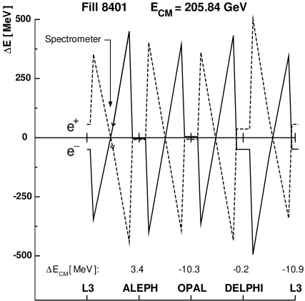
Figure 7: The RF sawtooth for a typical RF configuration in 2000. The electron beam is represented by the left-going solid line, the positron beam by the right-going dotted line. The locations of the experiments and the LEP spectrometer are indicated. $\Delta E=0$ corresponds to the average beam energy of LEP. $\Delta E_{\mathrm{CM}}$ is the correction to $E_{\mathrm{CM}}^{\mathrm{MOD}}$ at each IP due to RF effects.

The sawtooth variations are to first order anti-symmetric between the two beams, hence the correction to $E_{\mathrm{CM}}^{\mathrm{MOD}}$ is in general small. The calculation of the sawtooth is however rendered challenging by the instability of the RF system, the configuration of which varied from fill to fill as units broke and were repaired, and within fills, as units tripped. Additional inputs to the calculation come from knowledge of the absolute voltage calibration scale, and the alignment and phasing of the cavities.

During 2000 (and late in the 1999 run) dedicated fills were taken with single beams in order to perform $E_{\mathrm{b}}$ measurements with the energy spectrometer. Knowledge of the sawtooth is required to relate the local energy at the spectrometer, close to IP3, with $E_{\mathrm{b}}^{\mathrm{MOD}}$. The demands placed on the RF modelling are more exacting for these single-beam fills, as the result for an individual spectrometer measurement is directly sensitive to the absolute knowledge of the sawtooth. The spectrometer apparatus and analysis are discussed in sections 7 and 8.

5.1.1 Modelling the Sawtooth

The modelling of the energy corrections from the RF system is carried out by the iterative calculation of the stable RF phase angle $\psi_{s}$ which proceeds by setting the total energy gain, $V_{\mathrm{RF}}\sin\psi_{s}$, of the beams as they travel around the machine equal to the sum of all known energy losses. Here $V_{\mathrm{RF}}$ is the total RF accelerating voltage which is calculated using detailed measurements of the RF cavities, such as their voltage calibrations and their longitudinal misalignments. When available, the measured value of the synchrotron tune, $Q_{s}$, and the difference in horizontal displacement between the beams as they enter and leave the experimental IPs, are used to constrain energy variations due to the overall RF voltage scale and RF phase errors. (A full discussion of the synchrotron tune and its relationship to energy loss is given in section 9.)

The model of the RF system described above has been used to calculate the centre-of-mass energy corrections due to the RF system parameters for the whole of LEP 2 running. Its calculation of the energy loss in the LEP arcs, however, treats each arc as a single entity, rather than considering each magnetic component individually. For the spectrometer studies, a more detailed model has been developed based on the MAD program [24]. This model incorporates the detailed measurements of the RF cavities, on top of the complete specification of the LEP magnetic lattice[15]. Such an approach allows the calculation of the beam energy at any point in LEP, not just at the IPs. This feature permits the performance of the model to be studied through comparison with BPM data in the LEP arcs, which are sensitive to the effective $e^{+}e^{-}$ energy difference. The technique is illustrated in figure 8, where the energy offset between the electron and positron beam is clearly seen for two different RF configurations. A comparison of the two sawtooths allows the parameters of the system to be determined, in particular the net RF phase error at any LEP IP. Two experiments performed late in the 2000 run, in which the RF at each IP was powered down and up in turn, have been used to calibrate the method.

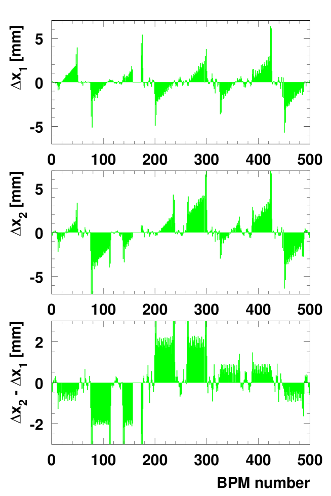
Figure 8: An example of the difference between electron and positron orbits ($\Delta x_{i}$ vs BPM number) for two different RF configurations (configuration 1 top; configuration 2 middle). IPs 2,4,6 and 8 are situated close to BPMs 60, 190, 310 and 440 respectively. The energy sawtooth is clearly visible. The difference of the two orbit differences is displayed on the bottom plot. The step changes reflect the different energy gains at the four IPs for the two configurations. Note that the orbit information is missing between BPMs 160 and 176.

The average corrections for all of the LEP 2 running are shown in table 6. Comparisons made between the two models at selected energy points show agreement to within 1 MeV.

Year	’96		’97	’98	’99				’00
$E_{\mathrm{CM}}^{\mathrm{nom}}$ [GeV]	161	172	183	189	192	196	200	202	205	207
IP 2 (L3)	19.8	19.4	8.2	6.0	8.8	8.2	8.0	8.0	3.4	3.0
IP 4 (ALEPH)	-5.6	-5.8	-10.8	-9.2	-12.6	-14.0	-13.8	-13.0	-11.0	-9.8
IP 6 (OPAL)	20.3	19.8	5.6	-2.6	-5.8	-5.2	-5.4	-4.4	-0.6	0.0
IP 8 (DELPHI)	-9.4	-8.4	-13.2	-10.4	-17.2	-16.0	-15.0	-14.0	-11.4	-9.8

Table 6: The luminosity-weighted RF corrections to $E_{\mathrm{CM}}^{\mathrm{MOD}}$ in MeV at each IP for each nominal energy point.

5.1.2 Error Assignment on the RF Corrections

The error assignment for the RF $E_{\mathrm{CM}}$ corrections arises from the following considerations:

• Any discrepancy between calculated and measured control variables, such as the $Q_{s}$ or the horizontal beam displacements, indicates imperfections in the model. For instance, discrepancies in the $Q_{s}$ reveal a lack of knowledge of the overall voltage scale or a phase error in the RF system;

• From measurements made with a beam-based alignment technique [16], the locations of the cavities are only known with a precision of 1 mm;

• A small uncertainty comes from the unknown misalignments and non-uniformities of all the magnetic components of LEP. This contribution can be estimated by simulating an ensemble of machines with imperfections similar to those expected in LEP.

In all cases the range of values of the energy corrections obtained when allowing the machine parameters to vary over their allowed values is taken as the systematic error. The procedure is discussed in detail in [3]. It should be noted that those energy-loss uncertainties important for the understanding of the $Q_{s}$ and detailed in section 9 have negligible impact on the $E_{\mathrm{CM}}$ corrections at the IPs.

The total error on $E_{\mathrm{CM}}^{\mathrm{MOD}}$ from the RF correction is estimated to be 8 MeV for the 183 GeV, 189 GeV and 192 GeV energy points, and 10 MeV for all other running. The conservative assumption is made that these uncertainties are fully correlated between IPs and energy points.

The BPM data, such as those seen in figure 8, provide a very powerful constraint on the MAD model of the individual beam sawtooth at the spectrometer, which is an important ingredient in the analysis presented in section 8. The error on this calculation for the dataset of spectrometer measurements is estimated to be 10 MeV. This value is set by the uncertainty in applying the results of the calibration measurements, made at the end of the 2000 run, to the earlier spectrometer experiments.

5.2 Possible Electron Positron Energy Differences

The energy of the electron and positron beams are not expected to be exactly identical. Orbit differences lead to small differences in the integrated bending field seen by each beam. The main cause for orbit differences at LEP is the energy sawtooth that separates the orbits at the highest beam energies by up to a few millimeters in the horizontal plane. Due to the strong energy dependence of the sawtooth, the expected energy difference, which is smaller than 1 MeV at 50 GeV, can reach 3-4 MeV around 100 GeV, according to simulation. To cover this possibility an uncertainty of 4 MeV is assigned on $E_{\mathrm{CM}}^{\mathrm{MOD}}$.

5.3 Opposite-Sign Vertical Dispersion

Beam offsets at the collision point can cause a shift in the centre-of-mass energy due to opposite-sign vertical dispersion [3]. During operation beam offsets were controlled to within a few microns by beam-beam deflection scans. The dispersions were measured each year, and also calculated within MAD. The shifts in centre-of-mass energy are estimated to be less than 2 MeV. This value is taken as the systematic uncertainty, with a 50 % correlation between years.

6 Constraining the Magnetic Model with the Flux-Loop

Each of the main dipoles had a copper loop embedded in the lower pole. These were connected in series throughout each of the octants of LEP. The flux variation in each octant was measured by a digital integrator. This system constituted the flux-loop (FL) [17]. It is estimated that the FL sampled 96.5% of the total bending field. In the LEP 1 era, prior to the routine use of RDP, dedicated FL cycles were regularly performed. These included a polarity inversion of the dipoles in order to determine the remanent field. From these cycles, and through expression 1, the absolute energy scale at the Z was determined with $\sim 10^{-4}$ precision [18].

The need to extrapolate up to fields equivalent to $E_{\mathrm{b}}=100~{}\mathrm{GeV}$ implies that it is impractical to use the FL as a tool of absolute energy calibration at LEP 2. Instead ramps were made from fields corresponding to RDP energies, up to fields equivalent to 100 GeV and beyond. In the analysis the evolution of the (almost) total bending field, as measured by the FL, can be compared to that predicted by the NMR model, thereby providing a constraint of the LEP 2 energy scale.

6.1 Measurement Procedure and Datasets

Measurements using the FL system were carried out during dedicated experiments, without beam, in each of the years of LEP 2 running. In each measurement the excitation current was ramped through a series of increasing values, which mostly corresponded to the physics energy settings, and the readings of the FL recorded in each of the eight LEP octants. The corresponding values of the 16 NMRs were also recorded. A summary of the experiments is given in table 7. Measurements were made in the region of 41 to 61 GeV, that is, in the region where there are also RDP data, as well as at higher energies. Also given in table 7 is the corresponding highest equivalent beam energy used for each year. In 1996 several FL measurements were also made, with equivalent beam energies up to 86 GeV. These were analysed on-line and are not part of the datasets considered here.

The FL measurements used in the analysis are the averages over the individual measurements made in each of the eight octants of LEP. However, particularly in the later years, not all of the octants were fully functioning due to radiation damage. Also, as discussed in section 3.2, the number of available NMR probes at any one time varied for the same reason.

Year	Number of Ramps	Highest Equivalent $E_{\mathrm{b}}$ [GeV]
1997	5	101
1998	18	101
1999	18	103
2000	10	106

Table 7: The number of FL ramps made in each year, together with the corresponding highest equivalent beam energy measured in that year.

6.2 Fitting Procedure

Fits may be performed between the NMR probes and the FL in the well-understood region of 41–61 GeV. These fits can be used to predict the average bending field as measured by the FL at the settings corresponding to physics energies. If the NMR probes can predict the FL field, and if the beam energy is proportional to the total bending field, then it is a good assumption that the probes are also able to predict the beam energy in physics. The FL cannot be used to predict the beam energy in physics directly, since neither the slope nor the offset of the relationship between measured field and beam energy are known with sufficient precision to make the extrapolation needed over the $\sim 50$ GeV interval.

Two methods are used to make an estimate of any possible non-linearity, with beam energy, in the procedure used in calculate $E_{\mathrm{b}}^{\mathrm{NMR}}$ at physics energies.

In method A, for each FL excitation current the equivalent beam energy from the dipoles, $E_{\mathrm{b}}^{\mathrm{NMR}}$, is determined from the NMR probe readings and expression 5, using the values of $a^{i}$ and $b^{i}$ established from the RDP data. In the 41-61 GeV interval of each FL ramp this is fitted against $E_{\mathrm{b}}^{\mathrm{FL}}$, the equivalent energy as estimated by the FL, where

$$E_{\mathrm{b}}^{\mathrm{FL}}=c+dB^{\mathrm{FL}}.$$ (13)

Here $c$ and $d$ are the fit coefficients, and $B^{\mathrm{FL}}$ the FL reading averaged over all available octants. The fit results are then used to find $E_{\mathrm{b}}^{\mathrm{FL}}$ at high energy, and this is compared with the value from the NMRs.

In method B each NMR probe $i$ is used to make an estimate of the FL reading, $B^{\mathrm{NMR}\,i}_{\mathrm{FL}}$  through the linear relation

$$B^{\mathrm{NMR}\,i}_{\mathrm{FL}}=e^{i}+f^{i}B^{\mathrm{NMR}\,i},$$ (14)

where $e^{i}$ and $f^{i}$ are determined from a fit to $B^{\mathrm{FL}}$ in the range 41–61 GeV. These estimates, averaged over all available probes irrespective of which octants they are in, give a mean NMR prediction of the FL reading, $B^{\mathrm{NMR}}_{\mathrm{FL}}$. The difference between $B^{\mathrm{NMR}}_{\mathrm{FL}}$ and $B^{\mathrm{FL}}$ at high energy can be expressed as an energy through multiplying by the ratio of average slopes in expressions 5 and 14 ($\langle b\rangle/\langle f\rangle$), to give a measure of $E_{\mathrm{b}}^{\mathrm{FL}}-E_{\mathrm{b}}^{\mathrm{NMR}}$.

Both methods provide a comparison between the FL and the NMRs at high energy, and thus are sensitive to non-linearities in the magnetic model. The NMR data are however used in a different manner by the two procedures, and this provides robustness against, for example, fluctuations caused by the varying number of probes available at each measurement point.

6.3 Comparison of FL Results Using Different NMRs

A strong correlation is expected between the offsets $a^{i}$ and slopes $b^{i}$ in equation 5 from the RDP calibration, and the offsets $e^{i}$ and slopes $f^{i}$ in equation 14 from the FL. The fitted parameters for each NMR are shown in figure 9, and the expected correlation is visible. The average offset, $\langle e\rangle$, is $-79.35$ Gauss, with an RMS spread over the 16 values of 0.69 Gauss. This offset corresponds to the 7 GeV nominal beam energy setting at the start of the FL ramp. The average slope, $\langle f\rangle$, is 0.9810, with an RMS spread over 16 NMR probes of 0.0026. The field plates placed below the NMRs, in order to improve the uniformity of the field, cause the slope to be 2% different from unity.

The behaviour of the different NMRs can be seen in figure 10. This shows the differences between the FL estimate of the beam energy, calculated with method B, and the individual NMR estimates, $E_{\mathrm{b}}^{\mathrm{NMR}\,i}$, plotted against the corresponding probe residuals of figure 3. The comparison is made at a beam energy of 100 GeV. Again, a strong correlation is observed.

These studies show that the FL measurements behave in a similar way to the RDP measurements in terms of the results from individual NMRs and give confidence that the FL data can be used to constrain the linearity of the magnetic model.

Figure 9: The offsets (a) and slopes (b) of equations 5 and 14 comparing the field measured by each NMR probe with the RDP and FL measurements. The values shown are averages over all the FL measurements. There is one entry per NMR probe in each plot.

Figure 10: For each NMR probe, the difference between the FL energy, from method B, and that estimated from the NMR probe is plotted against the difference between the mean NMR energy, averaged over all probes, and that from the individual probe in physics running. The differences are calculated at a beam energy of 100 GeV

6.4 Variation of FL Results for Different Octants and Years

The FL results used in the standard analyses are the averages of the available individual measurements for each of the eight octants of LEP. The results for the individual octants using method A are shown in figure 11. The differences between the FL value for each octant and the NMR values are computed at a beam energy of 100 GeV. The values for each octant have also been evaluated separately for each of the four years in which there are data, and the errors shown in figure 11 are half of the difference between the maximum and minimum of these yearly values. The results are consistent between octants, and exhibit year-to-year stability. The values from individual octants span a range of approximately 10 MeV. The RMS of the mean values from different octants is 5.5 MeV.

In figure 12 the values of $E_{\mathrm{b}}^{\mathrm{FL}}-E_{\mathrm{b}}^{\mathrm{NMR}}$ from method B are shown as a function of time. Each entry corresponds to a single FL ramp and the data from each year are separated. The beam energy at which the differences are computed varies from year to year and is indicated on the plot. It represents the main value at which physics data were taken in the year. The error bars shown are the RMS values of the results from each of the NMR probes. It can be seen that there is no strong time dependence in the measurements.

Figure 11: The difference, in MeV, between the magnetic field measured by the FL and predicted by the NMR probes for each octant separately, using method A. The differences are calculated at a beam energy of 100 GeV.

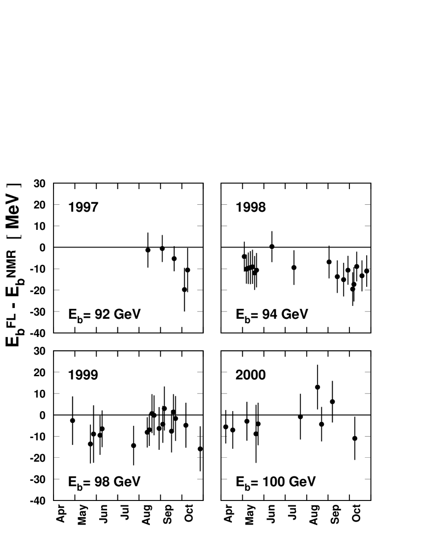
Figure 12: The difference, in MeV, between the magnetic field measured by the FL and predicted by the NMR probes for each of the FL measurements, using method B. The data are shown separately for each year.

6.5 Comparison of FL and NMR Energy Model Results

Table 8 lists the mean values of the $E_{\mathrm{b}}^{\mathrm{FL}}-E_{\mathrm{b}}^{\mathrm{NMR}}$ differences for each year, averaged over all the measurements in that year, from method A, for a beam energy of 100 GeV. The mean value averaged over all data is also included.

Table 9 presents the equivalent results from method B. A large part of the RMS scatter in the results comes from the different behaviour with energy of the NMR probes. Thus, if one or more of the NMR probes is not functioning for all, or part of, a particular measurement then this will increase the scatter.

The two fitting methods A and B are very compatible and the overall offset with respect to the energy model is small. However, the RMS values are smaller for method A, since the values used in this method are already averaged over the NMR probes.

Year	$E_{\mathrm{b}}^{\mathrm{FL}}$ $-$ $E_{\mathrm{b}}^{\mathrm{NMR}}$ [MeV]	RMS [MeV]
1997	2.8	4.4
1998	-4.5	6.1
1999	-3.3	6.3
2000	-4.7	12.2
All Years	-3.3	7.4

Table 8: Difference between the beam energy estimated by the FL and that using the NMR model at 100 GeV for each year separately, and also for all years together. The values given are from method A.

Year	$E_{\mathrm{b}}^{\mathrm{FL}}$ $-$ $E_{\mathrm{b}}^{\mathrm{NMR}}$ [MeV]	RMS [MeV]
1997	0.2	10.3
1998	-5.7	12.6
1999	-5.5	14.6
2000	-1.4	18.2
All Years	-4.2	17.7

Table 9: Difference between the beam energy estimated by the FL and that using the NMR model at 100 GeV for each year separately, and also for all years together. The values given are from method B.

6.6 Linearity in the High-Energy Region

The FL is the only device which allows a comparison with the NMR model measurements over a wide range of effective beam energies. The results of this comparison, averaged over all octants and all ramps, are presented, as a function of $E_{\mathrm{b}}$, in figure 13. The error bars shown are calculated from the spread of the individual FL measurements, over all years, at a given $E_{\mathrm{b}}$. The estimate from the FL is slightly lower than that from the NMR model and this difference grows somewhat with increasing beam energy. Also shown in figure 13 is a linear fit to the differences over the range 72 to 106 GeV equivalent beam energy. This fit gives a slope of -0.125 $\pm$ 0.028 MeV/GeV and an offset, at a beam energy of 100 GeV, of -5.2 $\pm$ 0.6 MeV. The $\chi^{2}$ for the fit is 13.2 for 5 degrees of freedom, giving a probability of 22$\%$. The errors are computed from the statistical spread of the FL measurements, and do not include any systematic effects.

Figure 13: The difference, in MeV, between the magnetic field measured by the FL and predicted by the NMR probes as a function of the nominal beam energy, using method A. Data from all years are used. For plotting, certain energy points have been averaged together. A linear fit to the differences is also displayed.

6.7 Robustness Tests and Systematic Uncertainties

Changes of the requirements in the fitting and extrapolation procedure of method A have been investigated. These include changing the minimum number of FL measurements in the range 41-61 GeV from 2 to 4, and changing the range of the fit in the low-energy region from 41-61 GeV to either 41-57 GeV or 50-61 GeV. All these modifications to the procedure give changes in the difference between the FL and the NMR model at 100 GeV, and averaged over all data, of 3 MeV, or less. Especially in the later years some of the octants did not always give FL data. Omitting each of the octants in turn from the analysis changes the mean value of $E_{\mathrm{b}}^{\mathrm{FL}}-E_{\mathrm{b}}^{\mathrm{NMR}}$ by less than 2 MeV.

There is very little redundant information in the FL measurements which allows a rigorous study of the possible systematic uncertainties to be performed. The accuracy of the device has previously been estimated to be about $10^{-4}$ [18], which corresponds to an uncertainty of 10 MeV at $E_{\mathrm{b}}=100~{}\mathrm{GeV}$. This is compatible with the RMS values seen in the octant-to-octant variations, and the results of the various extrapolation methods used (although part of this scatter is attributable to the behaviour of individual NMR probes).

The main uncertainty in the results comes from the assumption that the measured FL values are linear with the excitation current, and thus the beam energy. This can only be tested where there are RDP measurements, namely in the energy range 41-61 GeV. As a test of the linearity a special fit has been made to the RDP data for all years, using equation 5 as before, but excluding the 55 and 61 GeV points. A similar procedure has been carried out for the FL measurements using method A, and again not using the 55 and 61 GeV points. In both cases the fits are compared with measurements at 56.1 GeV, the mean value of the 55 and 61 GeV RDP data. These residuals are plotted in figure 14. The difference at 56.1 GeV between the RDP measurement and the model, and the FL measurement and the model, provides a linearity test over the sampled energy range. Scaling up the observed difference in order to extrapolate to a beam energy of 100 GeV gives 15 MeV, and this is taken as an estimate of the uncertainty in the linearity of the FL device at high energy.

Figure 14: Residuals from the NMR fits to the RDP data and FL data for all years, using method A. The error bars indicate the statistical scatter over the measurements. Only the data below 55 GeV are used in the fits.

It is known that a small fraction of the total bending field was not measured by the FL. This arose from three sources:

• The FL sampled only 98% of the total bending field of each dipole. The effective area of the FL varied during the ramp because the fraction of the fringe fields overlapping neighbouring magnets changed. The saturation of the dipoles, expressed as the change in effective length, was measured before the LEP startup on a test stand for different magnet cycles. The correction between 50 and 100 GeV is of the order of $10^{-4}$, corresponding to a 5 MeV uncertainty in the physics energy at 100 GeV, and scaling linearly with energy for other values.

• The weak dipoles matching the LEP arcs to the straight sections contributed 0.2% to the total bending field. Assuming that their field was proportional to that of the standard dipoles between RDP and physics energies to better than 1%, their contribution to any non-linearity in the model is around 1 MeV.

• The bending field of the double-strength dipoles in the injection region contributed 1.4% of the total. Their bending field has been measured by additional NMR probes installed in the tunnel, and is found to be proportional to the bending field of the main dipoles to rather better than $10^{-3}$, which gives a negligible additional systematic uncertainty.

The difference between FL and RDP residuals in figure 14 may be partly caused by these unmeasured contributions to the total bending field. To be conservative, however, they are considered as separate sources of uncertainty in the final error assignment.

6.8 Summary of FL Results

The central values of the FL analysis in the high-energy region are taken from the fit to the data of figure 13.

To determine the total systematic error to the FL measurement, it is assumed that the 15 MeV uncertainty arising from the non-linearity comparison is independent from the estimated 5 MeV uncertainty associated with the bending field lying outside the FL. Added in quadrature these give a value of 15.8 MeV at $E_{\mathrm{b}}=100~{}\mathrm{GeV}$. This systematic uncertainty is taken to be fully correlated as a function of beam energy and to increase linearly from a value of zero at 47 GeV, where the FL measurements are normalised to the RDP measurements. The range of FL measurements is from 72 GeV to 106 GeV, and this procedure gives an uncertainty which grows from 7.5 MeV to 17.6 MeV over this span.

7 The LEP Spectrometer

A project was initiated in 1997 to install an in-line energy spectrometer into the LEP ring with the goal of measuring the beam energy to a precision of $\sim 10^{-4}$ at $E_{\mathrm{b}}\ \sim 100~{}\mathrm{GeV}$. By replacing two existing concrete LEP dipoles with a single precisely mapped steel dipole, and installing triplets of high-precision BPMs on either side, the local beam energy could be measured as the ratio of the dipole bending field integral to the deflection angle. The full apparatus was installed close to IP3 and commissioned in 1999, and dedicated data taking took place throughout the 2000 run. A schematic of the spectrometer assembly is shown in figure 15.

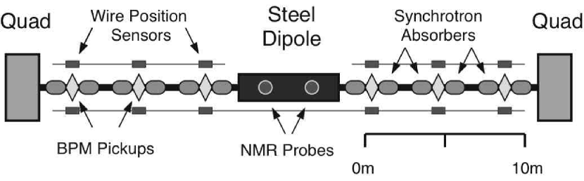
Figure 15: A schematic of the LEP spectrometer, situated between two quadrupole magnets close to IP3. The various components are discussed in the text.

While measuring the absolute deflection angle $\theta$ to the required accuracy is too great a challenge, a high-precision relative measurement can be performed by calibrating the spectrometer against a low-energy reference point, $E_{\mathrm{b}}^{\mathrm{ref}}$, well known through RDP, and measuring the change in bending angle, $\Delta\theta$, as the beam is ramped to the high-energy point of interest. Then the relative difference between the energy determination from the spectrometer, $E_{\mathrm{b}}^{\mathrm{\,SPEC}}$, and that predicted by the energy model, $E_{\mathrm{b}}^{\mathrm{MOD}}$, is given by:

$$\frac{E_{\mathrm{b}}^{\mathrm{\,SPEC}}\,-\,E_{\mathrm{b}}^{\mathrm{MOD}}}{E_{\mathrm{b}}^{\mathrm{MOD}}}\,=\,\frac{E_{\mathrm{b}}^{\mathrm{ref}}}{E_{\mathrm{b}}^{\mathrm{MOD}}}\,\frac{\int B\,\mathrm{dl}}{\int B\,\mathrm{dl^{\,ref}}}\,\left(1\,+\,\frac{\Delta\theta}{\theta_{0}}\right)\,-\,1,$$ (15)

where $\int B\,\mathrm{dl^{\,ref}}$ and $\int B\,\mathrm{dl}$  are the integrated bending fields at the reference point and measurement point respectively. The spectrometer dipole is ramped with the LEP lattice, and so its bending angle, $\theta_{0}$, remains approximately constant at a value of 3.77 mrad, and $\Delta\theta\,<<\,\theta_{0}$.

With a triplet lever-arm of roughly 10 meters, the spectrometer BPMs must have a precision of $\sim 1$ $\mathrm{\mu m}$ in the bending plane and be stable against mechanical and electronic drifts at this same level. This stability is only needed, however, for the few hours required to span the data taking at the reference point and the measurement point. How these problems were addressed is discussed in sections 7.3 and 7.4. The ratio $\int B\,\mathrm{dl}\,/\,\int B\,\mathrm{dl^{\,ref}}$ must be known to better than $10^{-4}$; the strategy pursued to achieve this is described in sections 7.1 and 7.2.

The beam energy at the spectrometer differs from the value of $E_{\mathrm{b}}$ averaged around the ring because of the RF sawtooth. Correcting for the sawtooth is an important ingredient in the spectrometer measurement. The same model was used as described in section 5.1.

7.1 The Spectrometer Dipole

The spectrometer magnet was a custom-built 5.75 m steel dipole similar in design to those used in the LEP injection region. It provided the same integrated bending field as the two concrete core dipoles it replaced, but over a shorter length, thereby maximising the space available for the BPM instrumentation. As a steel cored magnet it was also less susceptible to aging and had better stability under temperature variation. Thermal effects were further suppressed by water-cooling the excitation coils through an industrial regulation circuit which limited the rise in coil temperature, when ramping from $E_{\mathrm{b}}^{\mathrm{ref}}$ to high energy, to $3-4^{\circ}\mathrm{C}$. Temperature changes were monitored by several probes installed at a variety of locations.

Mounted directly in the gap of the spectrometer magnet under the beampipe were four NMR probes which continuously monitored the magnetic field strength. Two of these probes were optimised for measurements at fields equivalent to 60 GeV and below, the other two for fields corresponding to 40 GeV and above. The probes were situated in precision mounts similar to those used for the 16 NMRs of the magnetic model. During LEP operation radiation damage required that each probe had to be replaced two or three times during the year.

Field maps of the total bending field were performed in the winter of 1998-9 before the spectrometer magnet was installed in the LEP tunnel (the ‘pre-installation measurement campaign’), and again in 2001-02 after the magnet was removed following the LEP dismantling (the ‘post-LEP measurement campaign’). These maps were performed in a special mapping test stand as shown in figure 16. Using a precision motor stage instrumented with an independent NMR probe mounted on a carbon fiber mapping arm, the core magnetic field of the dipole was sampled every 1 cm along the longitudinal axis with an intrinsic relative precision of $10^{-6}$ for a variety of excitation currents and environmental conditions. The length scale was determined to a relative precision of $10^{-5}$ using a heterodyne ruler and verified with a laser interferometer. In the end-field region where the mapping NMR probe no longer locked due to the high field gradient, temperature-stabilized Hall probes, also mounted to the movable arm, were used to complete the field mapping. While these Hall probes had an intrinsic relative precision of $10^{-4}$, the end field represented only about 10% of the total dipole bending field, and thus a relative precision per map of $10^{-5}$ was achieved. With roughly 550 individual field readings taken per map, a single dipole map required roughly 30 minutes to complete.

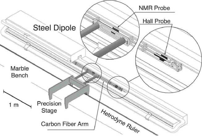
Figure 16: The magnetic mapping test stand, showing inset the components of the moving arm.

The field profile at 100 GeV is shown in figure 17, indicating the extent of the end fields. In both the mapping laboratory and the tunnel these end fields were truncated 0.5 m away from the dipole with mu-metal shields. Figure 17 also includes a zoom into the core region for a single map, to illustrate the uniformity of the field.

Figure 17: The longitudinal profile of the spectrometer dipole field at an excitation current corresponding to 100 GeV as measured by the mapping campaigns. Also shown is a zoom of the core region for a single map.

Using the results of the individual field maps, a model has been constructed to relate the total integral bending field of the dipole to the local field value measured by the four permanent reference NMR probes. A two-parameter fit is performed between the probes and the integral field for those excitation currents where each NMR was sensitive. A $\sim 10^{-4}\,/\,^{\circ}{\mathrm{C}}\,$ correction is included to account for the temperature dependence of the end fields, which are not tracked by the NMR probes. The model result is then taken to be the average of the individual predictions from all valid probe readings.

The relative residual differences between the measured integrated dipole field, for various datasets, and the model prediction after temperature correction, fitted to the post-LEP campaign data, are plotted in figure 18. Each point represents the mean value over all maps at an equivalent energy setting, and the error bar the RMS deviation over these maps.

The points corresponding to the post-LEP data (‘Arm, new Hall probes’) lie within $\pm 1.5\times 10^{-5}$ of zero, and each have RMS deviations of around $0.5\times 10^{-5}$. When looking at the pre-installation data (‘Arm’), however, an offset of $-8\times 10^{-5}$ can be seen. This is attributed to a bias associated with the Hall probe measurements of the original campaign. Hall probes used in these maps had a sampling area which was significant in size compared with the gradient of the end-field. This deficiency was rectified in the second campaign. This explanation was confirmed by making a sub-set of maps with the original instruments, the results of which are included in the figure (‘Arm, old Hall probes’) and are seen to agree with the pre-installation data.

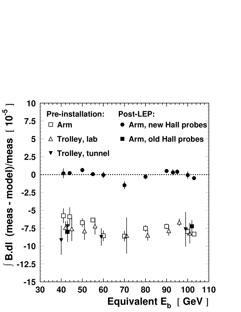
Figure 18: Relative residuals from the dipole magnet mapping campaigns, plotted against energy. Results are shown for all the mapping configurations discussed in the text. In all cases the model derives from a fit to the ‘Post-LEP: Arm, new Hall probes’ data. The horizontal positions of certain points have been slightly adjusted to aid clarity.

Additional maps were made with the arm displaced horizontally, in order to probe for any systematic effects which would arise from the finite sagitta of the beam. These show relative variations in the field integral of $10^{-6}$ for displacements of 1–2 cm, which is negligible for the energy calibration. Excellent stability is also observed for maps made with small vertical displacements.

Since the precision field mapping was performed in a magnetic test laboratory and not in the tunnel where the spectrometer operates, an additional in situ field-mapping technique was developed using an NMR probe and miniature flux coil mounted on a trolley which could be inserted directly into the LEP vacuum chamber. A laser interferometer was used to monitor the position of the trolley. The precision of this method is similar to that of the mapping-arm approach. Using this technique measurements were first made in the laboratory during the pre-installation campaign, with a section of vacuum chamber inserted into the dipole gap, and then again in the tunnel prior to the 1999 run. The residuals of the field integrals measured with this method are also shown in figure 18 (‘Trolley’). These results are seen to be consistent with each other and with the arm measurements of the pre-installation campaign, indicating that the field the beam sensed in the tunnel was the same as that measured in the laboratory. Because the sampling area of the flux coil was significant relative to the end-field gradient, these measurements shared a similar systematic bias with the Hall probes of the first campaign.

In the spectrometer energy analysis, detailed in section 8, it is the model fitted to the post-LEP data taken with the new Hall probes which is used to calculate the integrated bending field. As the mean values of the residuals are well determined at each magnet setting, these are applied as corrections to the model.

More information on the spectrometer dipole and the mapping campaigns and analysis can be found in [19].

7.2 Environmental Magnetic Fields

In addition to the bending field provided by the spectrometer dipole itself, in the LEP tunnel there were several other sources of magnetic fields which influenced the beam. The single largest effect came from the earth’s magnetic field, which was measured to be $\simeq 400$ mG in the LEP tunnel. Another contribution arose from the cables which provided current to drive both the main bending dipoles and the quadrupoles upstream from the spectrometer, which were mounted on the tunnel wall about 1 m from the beampipe. The magnetic fields produced by these currents were non-negligible and varied depending upon the nominal LEP beam energy and the specific details of the machine optics.

The ambient field strength in the tunnel was explicitly measured as a function of distance along the beamline while powering the main bending dipoles at several nominal LEP energy settings for both physics and polarisation optics. The data from these vertical field surveys are shown in figure 19. The large spikes in the field, visible on either side of the spectrometer magnet, correspond to the location of vacuum pumps which contained permanent magnets. Away from these spikes the absolute value of the field can be seen to decrease as the energy is raised, indicating that the contribution from the magnet cables is in the opposite sense to the earth’s field. The change in field has a stronger energy dependence for the polarisation optics.

Figure 19: Environmental magnetic field readings in the vertical direction as a function of longitudinal position along the spectrometer for the polarisation (a) and physics (b) optics. The dipole region is not shown. The large spikes are caused by permanent magnets situated in vacuum pumps.

Each spectrometer arm was equipped with a fluxgate magnetometer capable of 3-axis field measurements, situated immediately below the beampipe. These instruments allowed any variations in the ambient magnetic field to be monitored with time. Stable results are observed for all spectrometer data taking.

The effect of this ambient magnetic field was to bend further the beams while they traversed the BPM triplets. Without correction, an error on the calculation of the spectrometer bending angle of $\sim 10^{-4}$ is made when ramping to high energy. It is estimated that this field was monitored to a relative accuracy of 10%.

7.3 Beam-Position Measurements

Figure 20 (a) shows one of the six BPM stations of the spectrometer. Each BPM-block was mounted on a stable limestone base. Surveys carried out after installation showed, that on average, the blocks were well centred about their nominal positions with a RMS spread of 150 $\mathrm{\mu m}$ in the transverse plane. The horizontal position of each block could be adjusted by a stepping motor with a reproducibility of $<$ 100 $\mathrm{\mu m}$.

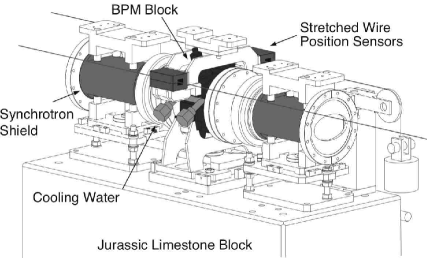
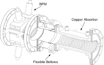
Figure 20: A spectrometer BPM station (a), and a cut away view of the BPM block and absorber (b). The various components are discussed in the text.

In order to ensure mechanical stability between low and high energy, copper shielding absorbers, as shown in figure 20 (b), were designed to shadow the BPM pickup blocks from the intense synchrotron radiation present in the LEP environment. During a ramp from $E_{\mathrm{ref}}$ to high energy the copper typically heated up by $15^{\circ}\mathrm{C}$, whereas the presence of the shielding and independent temperature regulation suppressed the rise in the blocks themselves to $\sim 0.2^{\circ}\mathrm{C}$.

Any residual movement from temperature or other effects was tracked by a stretched wire-position sensor system (WPS).

7.3.1 Geometry and Readout

Standard LEP elliptical BPM-blocks were used, with four capacitive button sensors. The dimensions and button layout are illustrated in figure 21. From the relative signal strengths of each button, $S_{i}$ ($i=1,4$), the BPM estimates of the beam position, $x_{\mathrm{BPM}}$ and $y_{\mathrm{BPM}}$, are calculated according to the following algorithm:

$$x_{\mathrm{BPM}}\>\propto\>\frac{(S_{1}-S_{3})\,-\,(S_{2}-S_{4})}{(S_{1}+S_{2}+S_{3}+S_{4})},$$ (16)

$$y_{\mathrm{BPM}}\>\propto\>\frac{(S_{1}-S_{3})\,+\,(S_{2}-S_{4})}{(S_{1}+S_{2}+S_{3}+S_{4})}.$$ (17)

To achieve the desired 1 $\mathrm{\mu m}$ resolution and stability, customised BPM readout-cards were developed in collaboration with industry, based on a design first used in synchrotron light source storage rings [20]. In the BPM electronics, the four analogue button signals from each BPM station were multiplexed into a common amplifier chain to reduce the effects of gain drifts on the measured beam position. The spectrometer BPM system, therefore, was not capable of turn-by-turn orbit measurements, but rather provided an integrated mean beam-position with a frequency response of around 100 Hz. Additional filtering was added to reduce noise and lower the overall frequency response to below 1 Hz. Gating allowed for the possibility of measuring both $\mathrm{e}^{-}$ and $\mathrm{e}^{+}$ positions during two beam operation, but more stable results were obtained without this feature enabled and with single beams. The cards were housed in a barrack some distance from the spectrometer, away from exposure to synchrotron radiation. A cooling system kept their temperature stable during operation to $0.1-0.2\,^{\circ}\mathrm{C}$.

Figure 21: Schematic of a LEP BPM-block and its button sensors, indicating the dimensions and the button numbering convention assumed in the text.

Prior to installation, the response of the BPM readout-cards was characterised in the laboratory using an electronic beam-pulse simulator. The stability of the card response was investigated against factors such as beam current and temperature. No dependencies that would introduce significant systematic effects during LEP operation [21] were found.

7.3.2 Relative-Gain Calibration

The response of the BPM readout differed between cards at the level of a few percent. In order to minimise errors on the measurement of the change in bending angle, online relative-gain calibrations were performed once or twice during almost all spectrometer experiments. These calibrations consisted of using four local corrector magnets to perform a series of beam translations and rotations, and minimising the triplet residuals in each arm separately, with the relative gains of the inner and outermost BPMs left as free parameters in the fit. The definition of the triplet residuals is illustrated in figure 22 for the bending plane, which also shows the BPM numbering definition. Residuals can also be constructed relating BPMs in different arms; this was done in order to fix the relative gain of the two triplets. An analogous procedure was used to determine the relative gains in the non-bending plane.

Figure 22: The definition of the BPM numbering scheme and bending plane triplet residuals.

Figure 23 shows a triplet residual for the same data before and after relative-gain calibration. The beam is undergoing rotations of up to 100 $\mathrm{\mu rad}$ and translations of up to 600 $\mathrm{\mu m}$. After calibration the triplet residual has a width of 0.3 $\mathrm{\mu m}$.

Figure 23: BPM relative-gain calibration. Displayed, as a function of time, are the beam movements in the calibration procedure, and the triplet residual before and after calibration. Also shown are the projections of the triplet residuals.

Repeated calibrations during individual spectrometer experiments indicate a relative-gain accuracy of $\simeq 0.2\%$, and suggest no dependence on beam energy or beam current. Larger variations are seen between experiments.

From calibrations performed close in time in both the horizontal and vertical planes, cross-talk effects between the x and y BPM readings can be studied. There are various possible sources of coupling between the x and y BPM readings, including an unintentional rotation of the BPM during installation, electrical cross-talk in the BPM readout system and non-linear terms in the BPM response, as discussed in section 7.3.4. The data show no indication of geometrical rotation, but do reveal electrical cross-talk of the order of 1% in some BPMs. Coefficients have been determined from these calibrations and then applied globally to all the experiments, resulting in small corrections.

7.3.3 Absolute-Gain Calibration

While the in situ calibration procedure described in the previous section can accurately determine the relative gain of the spectrometer BPMs, the overall absolute gain is still not constrained. To verify that the absolute-gain scale of the BPM system was sufficiently close to the assumed nominal value, spectrometer data were taken while the LEP beam energy was varied through changes in the RF frequency. An example of these measurements is shown in figure 24, in which the bending angle is clearly seen to evolve linearly with the change in RF frequency, $\Delta f^{\mathrm{RF}}$. From expression 7, and taking the spectrometer dipole field and local sawtooth correction to be stable throughout the $\mathrm{f^{RF}}$ changes, the dependence is expected to be

$$\frac{\Delta\theta}{\Delta f^{\mathrm{RF}}}\,=\,\frac{\theta_{0}}{\alpha_{c}\,f^{\mathrm{RF}}},$$ (18)

in the case where the assumed absolute gain is correct.

Figure 24: The change of bending angle measured in the spectrometer as the energy is varied through a manipulation of the RF frequency. The dependence is linear with a slope value consistent with expectations.

Eight separate absolute-gain measurements were performed in 2000, using both physics and polarisation optics. All measurements show good linearity between the change in bending angle and RF frequency, and consistency amongst the BPMs in the bending angle measurement. The ratio of the observed to the expected value of ${\Delta\theta}/{\Delta f^{\mathrm{RF}}}$ for these experiments has a mean value of $0.974\pm 0.036$, which is consistent with unity.

An independent constraint on the absolute-gain scale was obtained using the stepping motors to move each BPM-block in turn during LEP operation. The observed change in triplet residual could then be cross-calibrated against the physical movement measured by the wire sensors. These measurements also confirm the nominal gain to be correct with a precision of a few percent.

For the energy calibration measurements the nominal value of the gain scale is used with an uncertainty of $5\%$.

7.3.4 Non-linearities and Beam-Size Effects

Geometrical effects introduce higher-order terms in the BPM response which can be significant. Consider an idealised circular BPM with symmetrically distributed buttons at radius $a$, and a Gaussian beam of horizontal and vertical size $\sigma_{x}$ and $\sigma_{y}$ respectively, positioned at coordinates $x,y$. It can be shown that, in this case, the algorithm expressed in equation 16 gives for the BPM horizontal measurement [22]:

$$x_{\mathrm{BPM}}\>\propto\>x\,\left[1\,-\,\left(3\frac{\sigma_{x}^{2}-\sigma_{y}^{2}}{a^{2}}\,+\,\frac{x^{2}-3y^{2}}{a^{2}}\right)\right],$$ (19)

with a similar expression for the vertical coordinate. Therefore both the beam size and quadratic position terms affect the measurement.

The energy calibration with the spectrometer relies on determining the change in bending angle between $E_{\mathrm{b}}^{\mathrm{ref}}$ and high energy. Therefore what is relevant in equation 19 is how the higher-order terms change between the two energy points. The effect of the quadratic term can be suppressed by steering the beam at high energy as close as possible to the position it was at $E_{\mathrm{b}}^{\mathrm{ref}}$, and ensuring that this position is close to the centre of the BPM. This strategy also minimises any related errors arising from uncertainty in the gains.

The beam-size term is more important, as $\sigma_{x}$ grows with energy. (As $\sigma_{y}\,<<\,\sigma_{x}$ the change in the vertical beam size need not be considered.) Furthermore, the beam size changes across the spectrometer, because of the evolution of the LEP betatron function. With the polarisation optics, the estimated horizontal beam sizes at 50 GeV are 0.5 mm and 1.2 mm, for BPM 6 and BPM 3 respectively. At 90 GeV, these become 0.9 mm and 2.0 mm. Therefore, the bias to the position measurement over the energy step is different across BPMs, and for a non-centred beam an apparent change in bending angle results.

To examine the problem in detail, a simulation program has been developed to model the BPM response [22]. In the case of a circular BPM this gives results consistent with expression 19. For the elliptical BPMs of the LEP spectrometer, it is concluded that the systematic effects introduced in the energy measurement are small, provided that the beam passes within $\sim 1$ mm of the BPM centres and is re-centred to better than a few 100 $\mathrm{\mu m}$ between the two energy points.

7.4 The Wire-Position Sensor System

Given the stringent 1 $\mathrm{\mu m}$ requirement on the stability of the BPM system, additional instrumentation was installed to monitor independently the BPM positions. As shown in figure 15, the position of each BPM-block was measured in both the horizontal and vertical plane by a pair of stretched-wire capacitive-position monitors. One of the two wires spanned the entire 30 meter length of the spectrometer apparatus to give an independent reference line. A pair of sensors mounted on either side of each block, around 30 cm apart, allowed the effects of thermal expansion to be differentiated from relative transverse motion. Six additional sensors (not shown), mounted on invar  supports, placed on the limestone bases, provided reference measurements of the wire position, independently of the BPM-blocks.

The intrinsic resolution of the sensors was found to be better than $0.2\mathrm{\mu m}$. The absolute value of the gains and their stability with time were measured in the laboratory with a moving stage and laser interferometer [23].

During commissioning of the spectrometer, the WPS system was observed to be unexpectedly sensitive to the LEP environment. Figure 25 (a) shows the response of a reference sensor against time, throughout several successive LEP fills. Rapid positive changes in apparent position are seen, coincident with injection and ramp, followed by rapid decreases after beam adjustment. During the fills themselves apparent position drifts of several microns sometimes occur. Investigations showed this behaviour not to be physical; rather it was induced by a change in the dielectric constant of air, brought about by the ionising effects of the synchrotron radiation [23]. By installing additional synchrotron shielding, and taking care to centre the wires in the sensors, these jumps were suppressed, as is displayed in figure 25 (b), which shows the sensor reponse during several fills in which actual spectrometer measurements were performed.

Figure 25: The response of a reference WPS over two 12-hour periods before (a) and after (b) additional synchrotron shielding was installed, and the wire centred within the sensor. The vertical solid lines indicate the declared start-of-fill and the dotted lines indicate a beam dump. Note that (b) encompasses fills in which actual spectrometer measurements were performed.

Figure 26: BPM-block expansion as measured by the WPS system against temperature change during spectrometer measurements. The data are averaged over all six stations. A linear fit is superimposed.

In figure 26 is shown the BPM-block expansion, as measured by the WPS system, plotted against the change in block temperature for the spectrometer ramps from low to high energy in 2000. A clear linear dependence is seen, which agrees with the expected expansion coefficient of aluminium to $25\%$.

8 $E_{\mathrm{b}}$ Measurement with the LEP Spectrometer

8.1 Datasets

The dataset of experiments with usable spectrometer data at two or more energy points (multi-point) consists of 18 single-beam fills distributed uniformly throughout the 2000 LEP physics run. From these experiments, two largely overlapping samples are defined. The high-energy sample is made up of 17 fills in which spectrometer data were taken under stable conditions at both 50 GeV and high energy, typically 93 GeV but sometimes 90 GeV or 97 GeV depending on the available RF voltage. In 5 of these fills, the 50 GeV point was calibrated by RDP. The low-energy sample contains 8 fills with spectrometer data at two or more energy points between 41 GeV and 61 GeV, consisting of 21 such points in total. In this sample, 15 energy points in 6 fills were calibrated by RDP. In the high-energy sample, some data were also recorded at intermediate energies of 70 GeV and 80 GeV. In total 10 (5 $\mathrm{e}^{-}$, 5 $\mathrm{e}^{+}$) of the fills were taken with the physics optics, and 8 (5 $\mathrm{e}^{-}$, 3 $\mathrm{e}^{+}$) with the polarisation optics. The important details of the multi-point fills are summarised in table 10. This table also lists those fills used for the bending-field spreading (BFS) calibration, described in section 8.8.

Fill	Date	Optics	Particle	$E_{\mathrm{b}}$ of measurements [GeV]	Interest of experiment
					HE	LE	BFS
7129	11 May	Pol	$\mathrm{e}^{-}$	41 (P), 45 (P), 50 (P), 70, 93	$\bullet$	$\bullet$
7251	25 May	Pol	$\mathrm{e}^{-}$	41 (P), 45 (P), 50 (P), 70, 93	$\bullet$	$\bullet$
7391	8 June	Phy	$\mathrm{e}^{+}$	50, 93	$\bullet$
7491	18 June	Phy	$\mathrm{e}^{-}$	50, 93	$\bullet$
7519	21 June	Pol	$\mathrm{e}^{-}$	41 (P), 50 (P), 93	$\bullet$	$\bullet$
7676	6 July	Phy	$\mathrm{e}^{+}$	50, 93	$\bullet$
7833	20 July	Phy	$\mathrm{e}^{-}$	50, 93	$\bullet$
7835	20 July	Phy	$\mathrm{e}^{-}$	50, 93	$\bullet$
7929	26 July	Pol	$\mathrm{e}^{-}$	41 (P), 50		$\bullet$
7931	26 July	Phy	$\mathrm{e}^{+}$	50, 93	$\bullet$		$\bullet$
8221	21 Aug	Phy	$\mathrm{e}^{+}$	50, 90	$\bullet$
8224	21 Aug	Phy	$\mathrm{e}^{+}$	50, 90	$\bullet$
8368	4 Sept	Pol	$\mathrm{e}^{-}$	41 (P), 50 (P), 55 (P), 61, 90	$\bullet$	$\bullet$
8443	10 Sept	Pol	$\mathrm{e}^{+}$	50, 60, 70, 80, 90	$\bullet$	$\bullet$
8444	10 Sept	Pol	$\mathrm{e}^{+}$	50, 60, 70, 80, 90	$\bullet$	$\bullet$
8556	25 Sept	Pol	$\mathrm{e}^{-}$	45 (P), 50 (P), 55 (P), 93	$\bullet$	$\bullet$
8559	25 Sept	Pol	$\mathrm{e}^{+}$	50, 90	$\bullet$
8566	26 Sept	Phy	$\mathrm{e}^{-}$	50, 97	$\bullet$		$\bullet$

Table 10: Fills from the 2000 run used in the spectrometer analysis, indicating date, optics, particle type and energy points considered. In the ‘$E_{\mathrm{b}}$ of measurements’ column ‘(P)’ signifies that the energy was calibrated with RDP. ‘Interest of experiment’ indicates which of the datasets the fill belongs in: high-energy data set (‘HE’), low-energy data set (‘LE’), or BFS calibration (‘BFS’).

8.2 Characteristics of the Multi-Point Data

At each energy point in the multi-point fills, a period of data taking where the beams were centred and stable is chosen, and the spectrometer data analysed. Table 11 shows the mean and RMS variation of certain important parameters between measurements for the dataset, such as beam position and BPM-block temperature. It can be seen that for both the low and high-energy samples the beam was well re-positioned, and that the mechanical stability of the apparatus remained good. The change in bending angle when ramping between energies is found to be small, with typical values $|\Delta\theta|<1-2\,{\mu\mathrm{rad}}$. As a preliminary step to further analysis, corrections are applied to the BPM readings to account for mechanical shifts, as sensed by the WPS system, and to compensate for the extra bending in the spectrometer arms induced by the ambient magnetic field.

Quantity	Low energy		High energy
	Mean	RMS	Mean	RMS
Beam-position change in x [$\mathrm{\mu m}$]	-30	190	-57	145
Beam-position change in y [$\mathrm{\mu m}$]	-1	230	-43	184
BPM-block temperature change [${}^{\circ}\mathrm{C}$]	-0.07	0.06	0.16	0.15
BPM-block expansion [$\mathrm{\mu m}$]	-0.65	1.22	1.37	1.33
Dipole-core temperature change [${}^{\circ}\mathrm{C}$]	0.71	0.58	3.45	1.24

Table 11: Stability of key parameters in the spectrometer data set. The values refer to the change in parameter value between lowest and highest energy point considered. The BPM quantities are calculated by taking the station with the maximum excursion in each experiment.

The BPM triplet residuals are important figures-of-merit in monitoring the integrity of the spectrometer data. As explained in section 7.3.2, at a given energy point after gain calibration, these residuals are stable with a width of $<1\,\mathrm{\mu m}$. Furthermore, the calibration coefficients are equally applicable for other energy points within a given fill, giving good resolutions throughout. The central values of these residuals, however, are in general found to move between energy points. Figure 27 shows a typical example from fill 8443, where between 50 GeV and 90 GeV the triplet residuals are seen to move by $-1.7\,\mathrm{\mu m}$ in the left arm, and by $-4.7\,\mathrm{\mu m}$ in the right arm. Such triplet-residual shifts (TRS) indicate an effective relative movement amongst the BPMs, when ramping between energy points. These ‘movements’ cannot be real, as they are not tracked in sign or magnitude by the WPS system. Rather they must arise in the response of the BPM themselves, or in the readout electronics.

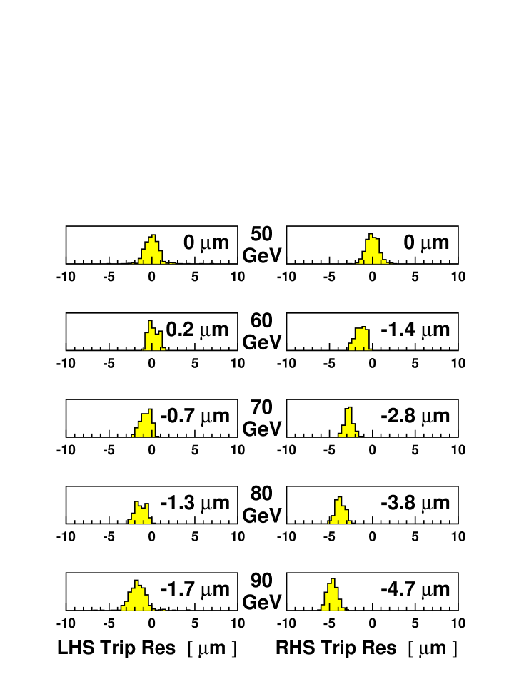
Figure 27: BPM triplet residuals for fill 8443. The gains have been calibrated and the triplet residuals centred at 50 GeV. Good resolution is observed at the other energy points, but accompanied by residual shifts. The inset numbers indicate the means of the distributions.

The characteristics of the TRS have been studied fill to fill. Figure 28 (a) shows the values of the shifts in both arms for ramps between 50 GeV and high energy. They are predominantly negative, and vary in magnitude. The means are $-1.54\pm 0.53\,\mathrm{\mu m}$ and $-2.90\pm 0.31\,\mathrm{\mu m}$ for the left and right arms respectively. A similar behaviour is observed at lower energy. Figure 28 (b) shows the mean value at each energy point of the TRS averaged over both arms ($\mathrm{\langle TRS\rangle}$), referenced to 50 GeV, for the full multi-point dataset.

Figure 28: Characteristics of the triplet-residual shifts: (a) shows the TRS in the left and right arms for the high-energy sample; (b) shows the mean TRS averaged over both arms ($\mathrm{\langle TRS\rangle}$), referenced to 50 GeV (asterix), as a function of energy, for the full multi-point dataset. The full points represent the polarisation optics and the open points the physics optics.

The exact origin of the TRS is not well understood. They are not correlated to temperature or to bunch current and have no dependence on particle type. The distribution in figure 28 (b) suggests a cause which varies approximately linearly with energy, thus disfavouring synchrotron radiation, and one which is more extreme for the polarisation optics. Variables which fulfil these criteria are the bunch size and length, which for the physics optics are similar between 50 GeV and high energy because of the routine use of wigglers, but in the case of the polarisation optics steadily increase. In dedicated experiments at a fixed energy TRS were indeed seen when wigglers were used to manipulate the beam parameters. BPM misalignments and the beam-size dependence discussed in section 7.3.4 might be one mechanism for the effect, but this is not proven. In the following analysis, the redundancy provided by the triplet of BPMs on either side of the spectrometer is exploited to make an internal calibration of the dataset, thereby minimising any biases brought about by the TRS in the energy determination.

8.3 Analysis of the High-Energy Data

8.3.1 Survey of the Raw Spectrometer Estimates

The energy model is used to calculate the mean beam energies at 50 GeV and the high-energy point. For each fill, the spectrometer is referenced to the model estimate at 50 GeV after applying a small correction to account for the known difference to the true energy seen in figure 2. The change of bending angle and integrated magnetic field is then used to determine $E_{\mathrm{b}}$ at high energy, and compared back to the model prediction, according to expression 15. When relating the mean beam energy to that determined at the spectrometer, sawtooth corrections are applied.

The procedure of normalising the spectrometer measurement to a reference energy means that in expression 15 the relative difference between the spectrometer and the model estimate, $E_{\mathrm{b}}^{\mathrm{MOD}}$, is insensitive to any uncertainties which scale with energy. This dependence is the case for all significant model contributions detailed in section 4 which are relevant in these measurements. To a very good approximation, therefore, it is non-linear systematics in $E_{\mathrm{b}}^{\mathrm{NMR}}$ alone which the spectrometer is constraining. For this reason, in the following the spectrometer results are compared with $E_{\mathrm{b}}^{\mathrm{NMR}}$.

Figure 29: Spectrometer results compared with the NMR model at high energy. For each measurement a spread is indicated showing the variation coming from the choice of 9 possible BPM combinations (‘Full range’), of which 3 specific cases are indicated (‘Outers’, ‘Inners’ and ‘Span’, defined as in figure 30).

The bending angle and changes thereof can be constructed from any combination of two BPMs in one spectrometer arm, and two BPMs in the other, giving nine such possibilities in total, each able to provide a separate determination of the energy. These determinations are not identical because of the TRS . Figure 29 shows the difference between the spectrometer and NMR model for all fills in the high-energy sample, where for each a spread is indicated, which corresponds to the variation from the different BPM combinations. This spread takes values between $\pm 16$ MeV and $\pm 59$ MeV. Of these nine combinations, three can be defined of particular interest:

• Outers – formed from the two outermost BPMs (6 & 5 together with 2 & 3);

• Inners – formed from the two innermost BPMs (5 & 4 together with 1 & 2);

• Span – formed by excluding the middlemost BPM (6 & 4 together with 1 & 3).

These combinations are illustrated in figure 30.

Figure 30: A schematic illustrating the three choices of BPM combinations used for determining the bending angle in the spectrometer energy analysis.

The energy determinations with each of these combinations are indicated in figure 29. It can be seen that in almost all cases the Outers give the lowest energy estimate of the possible combinations, and the Inners the highest, with the Span defining the median value. There are two exceptions: fill 8224 where the ‘Inner-Span-Outer’ hierarchy is inverted, and fill 7835 where other combinations give a much wider variation in result. These two fills have a large positive TRS in one arm and are anomalous within the sample. One other fill, 7251, exhibits a small positive TRS in one arm, but one which is countered by a more significant negative shift in the other arm. Fills 7835 and 8224 are dropped from further consideration at this stage, leaving a sample of 15 measurements sharing a common systematic behaviour. The nominal value of $E_{\mathrm{b}}$ at high energy for this sample is 92.3 GeV, averaged over the measurements.

The results in figure 29 are divided into electron and positron fills. There is an indication that the positron fills give a higher energy estimate than the electron fills, with a difference in the raw means of 36 MeV. Although $E_{\mathrm{b}}$, when averaged around the ring, must be the same within a few MeV for electrons and positrons, it is unsurprising that larger differences are seen in the spectrometer analysis. The RF sawtooth is anti-correlated between the two particle types, and so any residual error in calculating the correction will result in a separation between electrons and positrons of approximately twice this amount. Conversely, the mean value of the two samples will give a result which is rather robust against imprecisions in the sawtooth modelling.

8.3.2 Extracting $E_{\mathrm{b}}$ from a Global Fit

A priori it is not known which combination of BPMs gives the most reliable estimate of $E_{\mathrm{b}}$  as the TRS only indicate relative effective motion between the blocks. This question is best answered by studying the full ensemble of measurements. By considering the variation in results for the difference in spectrometer and energy model as a function of $\mathrm{\langle TRS\rangle}$, the BPM combination which gives the best stability can be identified. In addition an extrapolation can be attempted to the limit of zero systematic effect.

Figure 31 shows the spectrometer result, as compared to the NMR model, plotted against $\mathrm{\langle TRS\rangle}$. The plot is made separately for the Outers, Inners and Span results. Prior to plotting a correction has been made to minimize the difference between the electron and positron populations. This correction is one of three parameters (‘sawtooth’) in a least-squared fit made between the spectrometer results and $\mathrm{\langle TRS\rangle}$:

1. Offset – the extrapolated value of $(E_{\mathrm{b}}^{\mathrm{\,SPEC}}\,-\,E_{\mathrm{b}}^{\mathrm{NMR}})/E_{\mathrm{b}}^{\mathrm{NMR}}$ at $\mathrm{\langle TRS\rangle}$=0;

2. Slope – the gradient of $(E_{\mathrm{b}}^{\mathrm{\,SPEC}}\,-\,E_{\mathrm{b}}^{\mathrm{NMR}})/E_{\mathrm{b}}^{\mathrm{NMR}}$ with respect to $\mathrm{\langle TRS\rangle}$;

3. Sawtooth – the correction added to the electron results, and subtracted from the positron results, in order to compensate for residual errors in the sawtooth model.

The fit is made separately for each BPM combination. In the fit each spectrometer measurement is assigned a relative error of $17\times 10^{-5}$, which gives a $\chi^{2}/\mathrm{p.d.f.}$ of 1.06, 0.98 and 1.01 for the Outers, Inners and Span fits respectively. The fit results are superimposed in figure 31 and listed in the ‘Standard’ column of table 12.

Figure 31: Spectrometer results at high energy as a function of $\mathrm{\langle TRS\rangle}$, for different BPM combinations. The results of the fits described in the text are superimposed (solid line).

BPM	Fit parameters	Choice of input data
comb		Standard	Pol optics	Phy optics	Early data	Late data
	Offset	$-5.4\pm 14.9$	$13.7\pm 25.1$	$0.8\pm 22.1$	$-15.6\pm 19.9$	$4.7\pm 42.2$
Outers	Slope	$27.1\pm 5.6$	$32.2\pm 8.4$	$30.5\pm 9.5$	$24.3\pm 7.9$	$29.3\pm 16.6$
	Sawtooth	$14.1\pm 4.1$	$22.9\pm 6.0$	$6.1\pm 6.1$	$16.1\pm 6.7$	$12.7\pm 10.2$
	Offset	$-5.1\pm 14.9$	$13.9\pm 25.1$	$-0.2\pm 22.1$	$-13.1\pm 19.9$	$4.4\pm 42.2$
Inners	Slope	$0.7\pm 5.6$	$5.9\pm 8.4$	$3.5\pm 9.5$	$-1.4\pm 7.9$	$3.0\pm 16.6$
	Sawtooth	$13.3\pm 4.1$	$21.7\pm 6.0$	$5.7\pm 6.1$	$14.7\pm 6.7$	$12.5\pm 10.2$
	Offset	$-5.5\pm 14.9$	$13.4\pm 25.1$	$0.3\pm 21.6$	$-14.8\pm 19.9$	$4.1\pm 42.2$
Span	Slope	$13.9\pm 5.6$	$19.0\pm 8.4$	$16.9\pm 9.4$	$11.4\pm 7.9$	$15.9\pm 16.6$
	Sawtooth	$13.7\pm 4.1$	$22.5\pm 6.0$	$5.6\pm 6.0$	$15.4\pm 6.7$	$12.5\pm 10.2$

Table 12: Results of the global fit to the high-energy data. Results are given for the standard sample, and four example sub-sets. The units are as follows: Slope [$\mathrm{\mu}\mathrm{m^{-1}}\times 10^{-5}$], Offset [$\times 10^{-5}$] and Sawtooth [MeV].

It can be seen that, within the assigned errors, the energy estimate coming from the Inners shows no evidence of a significant dependence on $\mathrm{\langle TRS\rangle}$. The result from the Outers, on the other hand, shows a pronounced slope. The result from the Span fit lies between these two extremes. These fits suggest that there is little relative effective motion between the innermost pairs of BPMs, and it is the outermost BPMs in each arm, BPMs 6 and 3, which exhibit instability with respect to the other four. A calculation made under the hypothesis that all effective motion occurs in BPMs 6 and 3 predicts slope values of $26.9,\,0$ and $13.3\times 10^{-5}\,\mathrm{\mu m}^{-1}$ for the Outers, Inners and Span respectively, in very good agreement with the fit results to the data.

The fitted value of the offset in the global fit determines the spectrometer energy in the absence of TRS bias. It can be seen that all three of the combinations considered converge on the same value. The value corresponds to an offset of $-5\,\pm 14$ MeV with respect to the NMR model at a nominal energy of 92.3 GeV.

The returned value for the correction to the sawtooth model is 14 MeV, which is compatible with the 10 MeV uncertainty on the model estimated in section 5.1.

8.3.3 Robustness Studies

In order to probe the homogeneity of the dataset, and to cross-check the reliability of the errors coming from the global fit, the fit is repeated on various sub-samples of the data, namely:

• Division between polarisation and physics optics;

• Division between the first and second halves of the run;

• Samples with each of the 15 fills dropped in turn;

• Inclusion of the two anomalous fills 7835 and 8224;

• Division according to whether the TRS were more significant in the left or the right arms;

• Division into samples according to how well the beam was re-centred between energies, and according to the position of the beam orbits at the spectrometer;

• Excluding those fills common to the low-energy sample analysed in section 8.4;

• Excluding those fills with the largest fit residuals.

The results from several of these studies are given in table 12. The full variation of the key parameters are histogrammed in figure 32. The observed fluctuations are well-behaved, with the RMS of the offset distribution found to be $12.6\times 10^{-5}$. The largest deviations come from the smallest sub-samples, and are always within 1–2 sigma in uncorrelated error. The consistency between results from different BPM combinations remains good in all cases.

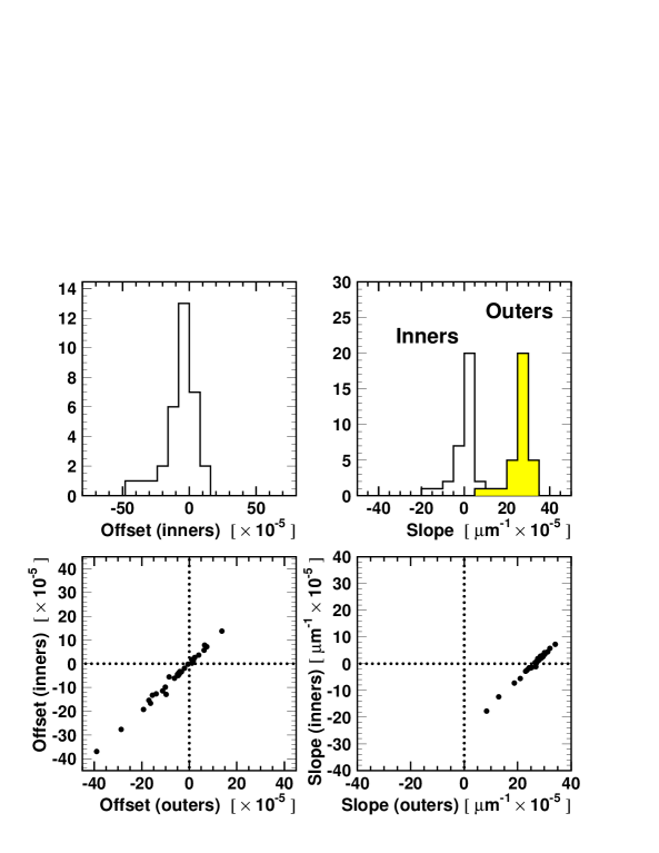
Figure 32: Variations in the fit result for the offset and the slopes for the inner and outer BPM combinations calculated from various combinations of fills in the high-energy sample. Each entry corresponds to a distinct subset, varying in size between 7 and 17 fills.

8.4 Analysis of the Low-Energy Data

The low-energy sample is important as it both allows the spectrometer’s performance to be evaluated in a regime where the energy is well known, and also provides an independent dataset in which to study the BPM behaviour and TRS characteristics.

Spectrometer energies are calculated as in the high-energy analysis for all data in the 41–61 GeV range listed in table 10. In fills with two low-energy points $E_{\mathrm{b}}^{\mathrm{ref}}$ is set at 50 GeV; in fills with three or more points the reference is chosen to be as close as possible to the mid-point of the full TRS excursion seen over the low-energy interval in that fill. Where available, the true energy is defined by actual RDP measurements; otherwise the energy model is used. As apparent in figure 2, there are residuals of 2–3 MeV between the fitted model and the energies as measured by RDP in the 41–61 GeV regime. Corrections are applied for these differences so that a comparison can be made between the spectrometer and the best possible estimate of the true energy, $E_{\mathrm{b}}^{\mathrm{\,TRUE}}$.

The fractional differences between the energy estimate from the spectrometer and the true energy are fitted against $\mathrm{\langle TRS\rangle}$. For this sample only two parameters are considered:

1. Offset – the value of $(E_{\mathrm{b}}^{\mathrm{\,SPEC}}\,-\,E_{\mathrm{b}}^{\mathrm{\,TRUE}})/E_{\mathrm{b}}^{\mathrm{\,TRUE}}$ at $\mathrm{\langle TRS\rangle}$=0;

2. Slope – the gradient of $(E_{\mathrm{b}}^{\mathrm{\,SPEC}}\,-\,E_{\mathrm{b}}^{\mathrm{\,TRUE}})/E_{\mathrm{b}}^{\mathrm{\,TRUE}}$ with respect to $\mathrm{\langle TRS\rangle}$.

As the low-energy sample is dominated by electron fills it is not possible to fit a correction to the sawtooth model. At low energy the sawtooth correction is significantly smaller, and consequently the expected precision of the RF model is much better. All data are included in the fit with their sawtooth correction fixed to that of the model. The mean residual of the two positron points is very close to zero, indicating that indeed there is no significant problem with the understanding of the sawtooth at these energies.

The data points and superimposed fit are shown in figure 33, and the results listed in table 13. The $\chi^{2}/\mathrm{p.d.f}$ of the fits are 1.10, 0.96 and 0.99 for Outers, Inners and Span respectively. These have been obtained by arbitrarily assigning an error to each point of $12\times 10^{-5}$, a smaller value than was required in the fit of section 8.3.2. This difference may be due to the increased significance of uncorrelated fill-to-fill imperfections in the sawtooth model at high energy.

Figure 33: Spectrometer results at low energy as a function of $\mathrm{\langle TRS\rangle}$, for different BPM combinations. Common symbols are used to designate measurements in the same fill. The results of the fits described in the text are superimposed (solid line).

BPM comb	Fit parameters	Result
Outers	Offset [$\times 10^{-5}$]	$5.6\pm 3.4$
	Slope [$\mathrm{\mu}\mathrm{m^{-1}}\times 10^{-5}$]	$21.5\pm 2.9$
Inners	Offset [$\times 10^{-5}$]	$6.1\pm 3.4$
	Slope [$\mathrm{\mu}\mathrm{m^{-1}}\times 10^{-5}$]	$-4.2\pm 2.9$
Span	Offset [$\times 10^{-5}$]	$5.9\pm 3.4$
	Slope [$\mathrm{\mu}\mathrm{m^{-1}}\times 10^{-5}$]	$8.8\pm 2.9$

Table 13: Results of the global fit to the low-energy data.

The slope values returned by the fit agree with those obtained at high energy. This shows that the same systematic behaviour is present in the two regimes, and that the low-energy sample can be used to assess the performance of the spectrometer at high energy.

The offset quantifies the agreement between the spectrometer estimate and the true energy when the TRS have been accounted for. This is found to be non-zero at a significance of almost two statistical sigma, suggesting a possible bias in the energy reconstruction of 3-4 MeV. No evidence is observed for an energy dependence in this offset. The bias, if real, is not understood; therefore a conservative error assignment is favoured over using the result to correct the high-energy fits.

The robustness of the result has been explored by isolating distinct sub-samples of points within the dataset, applying similar criteria to those used in section 8.3.3, and repeating the global fit. Distributions of the spread of results are shown in figure 34. Further investigations have been made varying the choice of reference point, the gains assumed in the BPM analysis, the RF sawtooth model and the value of the integrated dipole fields. From all of these studies it is concluded that the spectrometer correctly measures the relative energy change in the low-energy sample within a tolerance of $10\times 10^{-5}$. This uncertainty also encompasses the value of the fitted offset, plus one sigma.

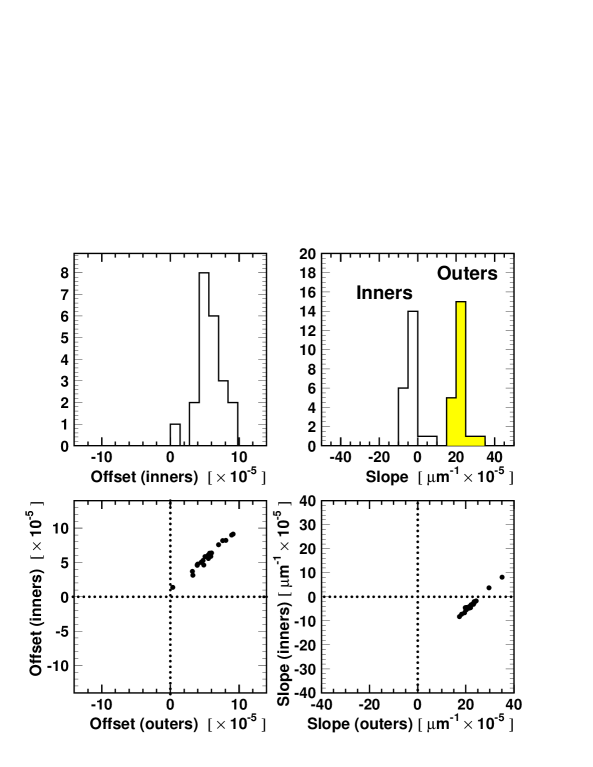
Figure 34: Variations in the fit result for the offset and the slopes for the inner and outer BPM combinations from various combinations of fills in the low-energy sample. Each entry corresponds to a distinct subset, varying in size between 4 and 13 energy points.

8.5 Systematic Error Assignment

8.5.1 Global Fit Results

The global fit offset result of $-5\times 10^{-5}$ at high energy provides the central value of the relative spectrometer energy determination with respect to the NMR model, a result which is the same for all BPM combinations considered, as is seen in table 12. The accompanying error from the fit of $15\times 10^{-5}$ is taken as the uncertainty associated with the scatter of the measurements.

The studies at low energy, presented in section 8.4, show a systematic behaviour fully compatible with that observed at high energy. The low-energy fit, however, suggests a possible small offset of the spectrometer measurements with respect to the true energy. On consideration of this, and the variations in this offset under different fit strategies, an error of $10\times 10^{-5}$ is assigned to represent the validity of the spectrometer performance as cross-checked in the 41–61 GeV regime.

8.5.2 Beam Size and BPM Non-Linearities

As discussed in section 7.3.4, the measured beam position, as conventionally calculated from the electrode signals of a BPM, ignores higher-order effects which introduce a potential systematic uncertainty into the spectrometer measurement. Contributions come from both the finite transverse beam size and from non-linear dependencies.

The variation in beam size has been calculated as a function of optics, longitudinal position in the spectrometer, and energy. The mean transverse offsets of the beam from the BPM centres, as estimated from consideration of the beam orbits of the measurements, and knowledge of the BPM alignments within the spectrometer, are found to be less than 1 mm. A simulation of the BPM response is then used to determine the change in apparent positions, and thus beam angle, with the variation in beam size for the measurements. From this study a relative error of $4\times 10^{-5}$ is assigned to the global energy determination.

As is seen in table 11, the beam was reliably re-positioned between low and high-energy measurements, with a spread of less than 200 $\mathrm{\mu m}$. This is sufficient to render non-linear effects negligible.

8.5.3 Knowledge of the BPM Gains

The dataset has been reanalysed changing the assumed scale of the BPM gains by $\pm 5\%$, and the global fit repeated. Variations of $0.5\times 10^{-5}$ are seen in the result. This weak dependence on the knowledge of the gains is a consequence of the care taken at high energy to re-steer the beam close to its low-energy position.

8.5.4 Knowledge of the Dipole Bending Field

The standard analysis is based on values of the integrated bending field derived from a model fitted to the data of the post-LEP mapping campaign. The analysis has been repeated using the model based on the pre-installation campaign data. This results in a change of the offset of $+1.5\times 10^{-5}$. Other models considered, relying on different fit strategies, and alternative magnet temperature corrections, give smaller variations. The difference between the pre-installation and post-LEP based results is taken as the error arising from bending field uncertainties.

8.5.5 Knowledge of the RF Sawtooth

At high energy the sawtooth correction is an important input in relating spectrometer measurements to the NMR model. The division of the dataset into nearly equal numbers of $e^{-}$ and $e^{+}$ fills, and the high degree of anti-correlation of the correction between the two particle types, enables the validity of the sawtooth model to be assessed, and in turn ensures that the energy determination from the global fit is largely insensitive to model imperfections.

Results have been obtained using both sawtooth models described in section 5.1, and using alternative tunings of each model. From these studies an uncertainty of $5\times 10^{-5}$ is assigned.

8.5.6 Uncertainty in Corrections to the Bending Angle Calculation

Prior to the calculation of the bending angle, corrections were applied from the WPS system to account for movements in the BPM-blocks. A further correction was applied for the effect of the ambient magnetic field on the beam trajectory. As part of the systematic error analysis these corrections are removed in turn, and the global fit is repeated. The results are shown in table 14.

BPM	Fit parameters	BPM correction dropped
comb		WPS movements	Ambient field
	Offset	$-14.5\pm 10.5$	$-10.1\pm 17.6$
Outers	Slope	$23.6\pm 4.0$	$32.2\pm 5.4$
	Sawtooth	$14.6\pm 4.1$	$14.1\pm 4.1$
	Offset	$-14.0\pm 10.5$	$-13.2\pm 17.6$
Inners	Slope	$-2.7\pm 4.0$	$1.8\pm 5.4$
	Sawtooth	$14.2\pm 4.1$	$13.6\pm 4.1$
	Offset	$-14.1\pm 10.5$	$-13.4\pm 17.6$
Span	Slope	$10.5\pm 4.0$	$13.7\pm 5.4$
	Sawtooth	$14.3\pm 4.1$	$13.7\pm 4.1$

Table 14: Results of the global fit to the high-energy data with each of the two corrections to the BPM readings removed in turn. The units are as follows: Offset [$\times 10^{-5}$], Slope [${\mathrm{\mu}\mathrm{m^{-1}}}\times 10^{-5}$] and Sawtooth [MeV]. The results should be compared to the ‘Standard’ column in table 12.

The fit error in both cases is different from that coming from the standard treatment. This is because the corrections move both the energies and the values of $\mathrm{\langle TRS\rangle}$ for each fill. For individual measurements the effect of the ambient field correction is larger than is apparent from this table. For results determined with the Outers and the polarisation optics, for instance, the correction is $\sim 25\times 10^{-5}$. However, a correlated correction is made at the same time to $\mathrm{\langle TRS\rangle}$, in such a manner that the resulting variation in the global fit results is much smaller. With no ambient-field correction, the consistency in the offset result for the different BPM combinations is degraded.

Following the discussion in sections 7.2 and 7.4, systematic errors corresponding to 10% and 25% of the full shift are assigned for the ambient-field and WPS corrections respectively.

8.6 Spectrometer Result at High Energy

The component uncertainties in the energy determination using the spectrometer are summarised in table 15, together with the total, under the assumption that the contributions are uncorrelated.

Contribution	Value
	[ $\times 10^{-5}$ ]
High-energy scatter	15.0
Validity at low energy	10.0
Beam size	4.0
BPM gains	0.5
Integrated dipole field	1.5
Sawtooth model	5.0
WPS correction	2.2
Ambient bending field	0.7
Total	19.3

Table 15: Summary of the error contributions to the spectrometer determination of the relative difference of $E_{\mathrm{b}}$ with respect to the energy model.

The spectrometer measures the following offset with respect to the NMR model at a nominal $E_{\mathrm{b}}$ of 92.3 GeV:

$$(\,E_{\mathrm{b}}^{\mathrm{\,SPEC}}-E_{\mathrm{b}}^{\mathrm{NMR}}\,)_{\,92\,\mathrm{GeV}} = -4.9\,\pm\,17.8\>\mathrm{MeV}.$$

8.7 Spectrometer Data at Intermediate Energies and in 1999

Table 10 lists four fills with spectrometer data taken at a nominal energy of 70 GeV. These may be analysed to provide a spectrometer result in this intermediate energy regime.

The sample of 70 GeV fills is too small to allow an independent study of the TRS behaviour. Instead, any systematic bias is corrected for using the slope results of the standard fit to the high-energy data. In fact, as can be observed from figure 28 (b), the $\mathrm{\langle TRS\rangle}$ evolution between 50 GeV and 70 GeV is rather small. Furthermore, in two of the fills, data at 60 GeV are used to define the reference point, as this choice further suppresses the TRS systematic.

The four fills give consistent results and are therefore combined to give a mean energy determination from the spectrometer at 70 GeV. The accompanying error from the sawtooth model is assigned to be half of the value of the applied correction. The other components in the uncertainty are estimated as for the high-energy data. The resulting offset between the spectrometer and the NMR model is found to be:

$$(\,E_{\mathrm{b}}^{\mathrm{\,SPEC}}-E_{\mathrm{b}}^{\mathrm{NMR}}\,)_{\,70\,\mathrm{GeV}} = -0.6\,\pm\,9.7\>\mathrm{MeV}.$$

The correlation with the measurement at 92.3 GeV is dominated by the common uncertainty arising from the verification of the spectrometer performance in the low-energy sample, and is estimated to be 75%.

This 70 GeV result is used in section 10, together with the measurement at 92.3 GeV, to constrain any evolution of non-linearity of the NMR model with energy. The 80 GeV points in fills 8443 and 8444 have not been analysed because of large TRS systematics and a very high correlation with the measurements at the other energy points.

During the latter period of the 1999 run, data were taken at low and high energy in order to commission the spectrometer. The stability of the operating conditions were significantly inferior to 2000. Furthermore, all the experiments were made with an electron beam, not allowing constraints to be placed on the sawtooth model for this year. For these reasons, no quantitative results are presented. The comparison of the spectrometer measurements with the true energy as a function of $\mathrm{\langle TRS\rangle}$ in figure 35 shows, however, that the behaviour at low energy for each BPM combination appears to be very compatible with that observed in 2000, although the points exhibit a larger scatter. Figure 36 indicates that the results at high energy are also consistent. (Some of these data have positive TRS in one arm, which when averaged with the negative values in the other arm, lead to smaller values of $\mathrm{\langle TRS\rangle}$ than in 2000.) This adds confidence for the 2000 analysis.

Figure 35: Spectrometer results in 1999 at low energy as a function of $\mathrm{\langle TRS\rangle}$, for different BPM combinations. Common symbols are used to designate measurements in the same fill. The bold lines show the results of linear fits made to the data. Superimposed as dashed lines are fits to the 2000 data set.

Figure 36: Spectrometer results in 1999 at high energy as a function of $\mathrm{\langle TRS\rangle}$, for different BPM combinations. Superimposed as dashed lines are fits to the 2000 data set.

8.8 Measurement of the BFS Boost with the Spectrometer

In addition to constraining the magnetic extrapolation, the spectrometer is also used to calibrate the bending-field spreading (BFS) boost. In both fills 7931 and 8566, after the usual spectrometer measurements had been made at high energy, a BFS boost was then applied. This action induced a noticeable change of bending angle in the spectrometer. In order to minimize BPM-related systematics, the RF frequency was increased so as to introduce a known energy change of opposite sign to the BFS, and thereby return the bending angle to close to its original value. Care was also taken to re-steer the beam back to its position prior to the boost. The residual change in bending angle is measured, and from this and the change in $\mathrm{f^{RF}}$  the effect of the BFS boost is determined.

The results of the experiments are shown in table 16, giving both the nominal and measured values of the boost applied. In calculating the systematic error, contributions are considered from the variation in result with BPM combinations; from a $5\%$ uncertainty in the absolute-gain scale; through any variation in relative gains seen in the online calibrations within the fill; and from a $1\%$ error in the momentum compaction factor. Because of time constraints, the beam was significantly less well re-centred in fill 8566 than in 7931, and this explains the difference in precision between the experiments. Both measurements, however, show the value of the BFS boost to be consistent with expectations.

Fill	Nominal BFS	Measured BFS
7931	219 MeV	213.5 $\pm$ 7.8 MeV
8566	297 MeV	304.1 $\pm$ 33.5 MeV

Table 16: Results for the BFS calibration experiments.

9 $E_{\mathrm{b}}$ Measurement with the $Q_{\mathrm{s}}$ Fit

The combined effects of synchrotron radiation loss, and the boost from the RF system, leads to particles undergoing longitudinal oscillations. The frequency of these oscillations is dependent on the particle energy. An analysis based on measurements of the oscillation frequency, therefore, offers an alternative way to determine $E_{\mathrm{b}}$ and constrain the energy model.

9.1 Energy Loss and Synchrotron Oscillations

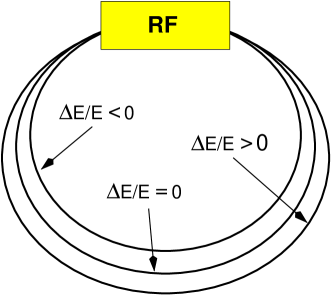
Figure 37: Change of orbit length ($\Delta L$) for particles with energy deviation ($\Delta E$) in an accelerator with a single RF cavity (left). Accelerating voltage as a function of phase; particles with different energies arrive at different phases, thus seeing a voltage different from that needed to compensate the nominal energy loss per turn (right).

Consider the case of a beam of energy $E_{\mathrm{b}}$, experiencing an energy loss per turn in the dipole magnets of $U_{0}$, as given by expression 3. This energy loss is restored by the RF system, which, for the purposes of discussion, is taken to be a single cavity as shown in figure 37.  The voltage provided by the cavity to the arriving beam can be expressed as

$$V(\psi)=V_{\mathrm{RF}}\sin\psi,$$ (20)

where $V_{\mathrm{RF}}$ is the peak voltage provided by the system and $\psi$ the phase. The stable phase angle, $\psi_{s}$, of particles with the nominal energy, is defined by the condition $U_{0}=e\,V_{\mathrm{RF}}\sin\psi_{s}$. Particles with lower-than-nominal energy follow a shorter path length and, in the ultra-relativistic regime, arrive at an earlier time in the RF cycle, therefore experiencing a larger energy boost than particles at $\psi_{s}$. The converse is true for particles with higher than nominal energy. These effects lead to synchrotron oscillations of angular frequency $\Omega$. Assuming that the amplitude of oscillations is small, and the damping due to synchrotron radiation is negligible, it can be shown [25] that:

$$\Omega^{2}~{}=~{}\omega_{\mathrm{rev}}^{2}\left(\frac{\alpha_{c}h}{2\pi E_{\mathrm{b}}}\right)~{}e~{}\frac{dV}{d\psi}(\psi_{s}),$$ (21)

where $\omega_{\mathrm{rev}}$ is the angular revolution frequency, $\alpha_{c}$ is the momentum compaction factor and $h$ the harmonic number of the accelerator, that is the ratio between the RF frequency and the revolution frequency (31320 in the case of LEP).

The synchrotron tune, $Q_{s}$, is defined as the ratio of the oscillation frequency to the revolution frequency. Expression 21, together with the definition of the stable phase condition, gives the following relation:

$$Q_{s}^{2}=\left(\frac{\alpha_{c}h}{2\pi E_{\mathrm{b}}}\right)\sqrt{e^{2}~{}V^{2}_{\mathrm{RF}}-U_{0}^{2}}.$$ (22)

In principle, therefore, fitting expression 22 to measurements of the synchrotron tune at different RF voltages enables the beam energy to be determined. In practice, however, this expression is inadequate for energy calibrations of the required precision. It neglects energy losses in the quadrupoles, correctors and from other sources. Further corrections are necessary to account for the particular distribution of RF cavities at LEP and the possibility of large-amplitude oscillations. These refinements are discussed in section 9.3.

9.2 Measurement Procedure and Datasets

The determination of the $Q_{s}$ was based on a measurement of the phase between a bunch and the RF frequency. Figure 38 shows a block diagram of the LEP bunch phase monitoring system. The summed signal from a four-button BPM was processed with band pass filters centred at the RF frequency, amplifiers and an automatic gain control (AGC) loop. The phase of the resulting signal was compared to the RF frequency (mixer), and the output fed into a spectrum analyser. The $Q_{s}$ peak in the resulting Fourier-analysed spectrum was located manually  with a typical accuracy of 0.0003. In general, the signal was averaged over several turns and over all bunches.

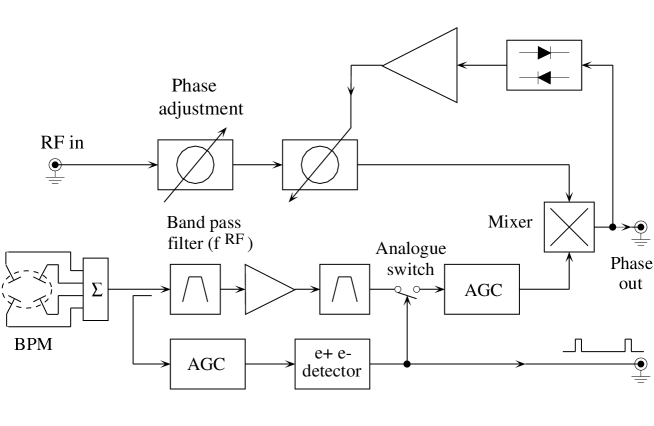
Figure 38: A schematic block diagram of the LEP synchrotron oscillation detector.

In a $Q_{s}$ energy calibration experiment, measurements were first made at one or more low-energy points, before ramping to high energy. The purpose of the low-energy measurements was to enable the absolute scale of the RF voltage to be fixed through cross-calibration against the energy model in a regime where the model is known to be reliable. At each energy point the total RF voltage, $V_{\mathrm{RF}}$, was varied over the same range, stepping between the lowest value compatible with stable operation at high energy, to the maximum available. The need to span a significant range in $V_{\mathrm{RF}}$ dictated that the choice of high-energy point, most usually 80 GeV, was typically somewhat lower than that attainable by the full RF system during physics operation. At each value of $V_{\mathrm{RF}}$ the synchrotron tune was measured. Data from a typical $Q_{s}$ experiment are shown in figure 39.

Figure 39: Measured $Q_{s}$ is shown against $V_{\mathrm{RF}}$ for different beam energies. The calibration set for the voltage calibration factor is indicated, together with the high-energy data.

Energy calibration experiments using $Q_{s}$ were made in 1998, 1999 and 2000 and are listed in table 17. In total six fills were used to measure $E_{\mathrm{b}}$ at high energy. Other fills were used to constrain uncertainties in the higher order corrections to the model. All but one of these were made with single beams of positrons. (Fill 5128 was made with positrons and electrons simultaneously.) The choice of optics was 102/90 for all experiments apart from 8445, which was performed with 101/45. The bunch currents were set low, with typical values of $50\,{\mathrm{\mu}\mathrm{A}}$, so as to minimise the parasitic mode energy loss discussed in section 9.3.2.

Fill	Date	$E_{\mathrm{b}}$ of measurements [GeV]	Interest of experiment
5128	4 Sept ’98	66, 91	Energy calibration
5981	24 July ’99	61	Parasitic mode loss
6114	13 Aug ’99	50, 55, 61, 81	Energy calibration
6338	15 Sept ’99	50, 55, 61, 80	Energy calibration
7456	14 June ’00	42, 45, 48, 50, 55, 61	Bending radius constraint
7832	20 July ’00	61	Parasitic mode loss
8315	29 Aug ’00	50, 55, 61, 80	Energy calibration
8445	10 Sept ’00	50, 55, 61, 65, 80	Energy calibration
8809	18 Oct ’00	50, 55, 61, 65, 80	Energy calibration

Table 17: List of $Q_{s}$ fills, giving the energy points analysed and the main purpose of the experiment.

9.3 The Improved Synchrotron Oscillation Model

9.3.1 RF Calibration and Distribution

The effective voltage seen by the beam can be significantly different from the sum of all individual nominal cavity voltages due to uncertainties in the voltage calibration, phasing errors, and longitudinal alignment errors. A crucial correction to expression 22 is therefore to replace $V_{\mathrm{RF}}$, the nominal total RF voltage, by $g\,V_{\mathrm{RF}}$, where $g$ is a correction factor to account for these effects.

Figure 40: Synchrotron tune as a function of total RF voltage as calculated with the MAD program for different RF configurations. The curve is a fit to the correct RF distribution using the model of equation 25.

The correction factor is determined separately for each experiment by fitting the final $Q_{s}$ model (see expression 25) to the low-energy data for different values of $g$, to find the factor which results in a beam energy in agreement with the energy model. Care is taken to use the same configuration of RF cavities and span of voltages at each energy point, so that this correction factor is applicable to the high-energy point of that experiment. The uncertainty in $g$ is taken from the scatter in results over the low energy points, and the central value from the average. The results for each experiment are shown in table 18. $g$ is typically found to be within a few percent of unity, with an uncertainty of $\sim$ 0.001.

Fill	$g$
5128	0.9499 $\pm$ 0.0006
6114	0.9805 $\pm$ 0.0009
6338	1.0006 $\pm$ 0.0008
8315	1.0054 $\pm$ 0.0009
8445	1.0064 $\pm$ 0.0005
8809	1.0030 $\pm$ 0.0002

Table 18: Fit results of the voltage calibration factor, $g$, for the 6 fills used in the $Q_{s}$ energy measurement.

Expression 22 is derived assuming that the RF voltage is distributed homogeneously around the accelerator. In LEP, however, the cavities were concentrated in the four straight sections. Investigations with the MAD program [24] show that $Q_{s}$ has a dependence on this distribution. This can be seen in figure 40 which shows $Q_{s}$ generated for a beam energy of 50 GeV with three different RF configurations: a typical case with the standard LEP RF distribution, a case where the same total voltage is concentrated at one point, and the limit of a homogeneous distribution where the voltage is distributed over the whole ring. The correct distribution can be adequately modelled by adding in expression 22 a term in $V_{\mathrm{RF}}^{4}$, controlled by a weighting coefficient $M$ of order $10^{-7}$. This is illustrated by the superimposed curve in figure 40.

When analysing the data, the value for $M$ is taken from fits to the appropriate MAD simulations. Any residual imperfections in this treatment are absorbed into the voltage calibration factor.

9.3.2 Total Energy Loss

Expressions 3 and 22 assume that the beam energy is fully supplied by the dipole field, and that all the energy loss arises through synchrotron radiation in the dipoles. As neither assumption is wholly valid, the total energy loss $U_{o}$ as used in equation 22 has to be replaced by

$$\tilde{U}_{0}=\frac{r\,C_{\gamma}}{\rho}(E_{\mathrm{b}}^{\mathrm{d}})^{4}\,+\,\sum\Delta U,$$ (23)

where $E_{\mathrm{b}}^{\mathrm{d}}$ refers to that part of the beam energy defined by the dipoles alone, and

$$\sum\Delta U\,=\,(\Delta U_{\mathrm{E_{\mathrm{b}}}}+\Delta U_{\mathrm{quad}})+\Delta U_{\mathrm{closed}}+\Delta U_{\sigma}+\Delta U_{\mathrm{cor}}+\Delta U_{\mathrm{\,PML}},$$

is the sum of all additional energy loss, which are explained in the following. The factor $r$ represents a correction to the inverse bending radius, and is discussed separately in section 9.3.3.

Quadrupole Effects

As discussed in section 4, the beam energy as set by the dipole field receives additional contributions, the most important of which is associated with off-centre trajectories in the quadrupoles. According to relation 2 the energy loss in the dipoles scales as $E_{\mathrm{b}}^{2}\,B^{2}$, where $B$ represents the dipole field. Therefore, in expression 23 the familiar energy-to-the-fourth power term is specified as being associated with the dipole field alone, and a correction $\Delta U_{E_{\mathrm{b}}}$, is added, where $\Delta U_{E_{\mathrm{b}}}/{U_{0}}\,=2\,(\Delta E_{\mathrm{b}}/E_{\mathrm{b}})$.

In addition to modifying the beam energy, beam offsets in the quadrupoles will result in synchrotron radiation in the quadrupoles themselves. For a transverse offset of $(x_{0},y_{0})$ this contribution to the turn-by-turn energy loss, $\Delta U_{\mathrm{quad}}$, goes as $E_{b}^{4}\,(x^{2}_{0}\,+\,y^{2}_{0})$. A beam of energy 80 GeV at an offset of 0.5 mm will lose approximately 0.2 keV in each of the 850 quadrupoles.

The net effect of additional contributions to the beam energy, and of synchrotron radiation in the quadrupoles, has been studied with the MAD program. Figure 41 shows how the relative energy loss from both sources varies with relative $E_{\mathrm{b}}$ changes induced by beam offsets. As expected, the dependence exhibits the superposition of a linear term, associated with $\Delta U_{E_{\mathrm{b}}}$, and a quadratic term, coming from $\Delta U_{\mathrm{quad}}$. The variation at high and low energy is sufficiently similar to allow a common parameterisation. This is then included in the $Q_{s}$ model to account for the offsets caused by $\mathrm{f^{RF}}$ manipulations, earth tides, and longer timescale geological distortions, as tracked by the $\mathrm{f_{c}^{RF}}$ evolution.

Figure 41: Variation of relative energy loss with relative energy change induced by beam offsets in the quadrupoles. The results are calculated with MAD for two energy points. A common parameterisation is superimposed. Note that during operation the relative energy change from beam offsets is typically $\leq 10^{-4}$.

Even when the global effects coming from these sources are subtracted, there remain significant local offsets from quadrupole to quadrupole, with typical RMS of 0.5 mm. These ‘closed orbit distortions’ are logged in BPMs close to the defocusing quadrupoles, and can be extrapolated to the focusing quadrupoles with knowledge of the local betatron function. These offsets are used to calculate the additional energy loss, $\Delta U_{\mathrm{closed}}$, from all the quadrupoles around the machine. Note that though fundamentally random in distribution, they contain a residual systematic component from the variation in horizontal position arising from the RF sawtooth.

A final addition to the energy loss arising from the quadrupoles is $\Delta U_{\mathrm{\sigma}}$, a contribution caused by the finite beam size. This is present even for beams which have no offset, and is proportional to $E_{b}^{4}\,(\sigma_{x}^{2}\,+\,\sigma_{y}^{2})$, where $\sigma_{x}$ and $\sigma_{y}$ are the horizontal and vertical beam sizes respectively. MAD is used to calculate the beam size at each quadrupole, so that the energy loss from this source may also be included.

Other sources of Synchrotron Radiation

Additional energy loss occurs through synchrotron radiation in the corrector dipoles. This contribution, $\Delta U_{\mathrm{cor}}$, is calculated taking as input the RMS scatter in the logged values of the settings around the ring.

Synchrotron radiation in the sextupole magnets leads to negligible energy loss.

Parasitic Mode Losses

After the synchrotron radiation in the bending dipoles, the so-called parasitic mode losses [26] are the largest contribution to the total energy loss. These arise from the impedance experienced by the beam from resistance in the vacuum chamber walls and from resonator-like structures.

For each particle, the energy loss per turn from this source is $\Delta U_{\mathrm{\,PML}}\,=\,2\pi\,e\,I_{b}\kappa_{||}\,/\,\omega_{\mathrm{rev}}$, where $I_{b}$ is the beam current, and $\kappa_{||}$ the longitudinal loss factor, which in turn depends on the longitudinal resistive impedance [27]. $\Delta U_{\mathrm{\,PML}}$ can be determined from the data by including the parasitic mode loss in the $Q_{s}$ description and fitting the model to the data at low energy over a range of different beam currents.

Figure 42 shows measurements of $Q_{s}$ as function of RF voltage at an energy of 61 GeV for two bunch currents of $10~{}{\mathrm{\mu}\mathrm{A}}$ and $640~{}{\mathrm{\mu}\mathrm{A}}$ for a fill in 1999. The difference in behaviour due to parasitic mode losses is clearly visible. A simultaneous fit to the data from five different bunch-current values yields a current dependent energy loss of $\Delta U_{\mathrm{\,PML}}/I_{\mathrm{b}}\,=\,(18.5\pm 2.0)$ MeV/mA. This result is confirmed by the analysis of a second experiment, conducted in 2000, which gives $\Delta U_{\mathrm{PML}}/I_{\mathrm{b}}\,=\,(20.7\pm 3.1)$ MeV/mA.

Figure 42: $Q_{s}$ as function of total RF voltage for two different bunch currents in fill 7831, showing the effect of the parasitic mode losses. The curves are individual fits to each dataset.

The longitudinal loss factor is expected to have some weak dependence on the bunch length, which itself varies with $Q_{s}$. Fits to the experiments with different bunch currents are not sensitive to this variation, due to correlations with other parameters. Therefore in parameterising the parasitic mode loss in the energy fits for a given dataset, a constant value of $\Delta U_{\mathrm{\,PML}}/I_{\mathrm{b}}$ is assumed, and the approximation taken account of in the error assignment. A dataset-dependent scaling factor is applied to account for the differences in bunch length with optics setting.

Summary

Energy Loss Mechanism	Energy Loss [MeV]
	50 GeV	61 GeV	80 GeV
Offsets in quads ($\Delta U_{\mathrm{E_{\mathrm{b}}}}+\Delta U_{\mathrm{quad}}$)	-0.1	-0.3	-0.9
Closed orbit distortions ($\Delta U_{\mathrm{closed}}$)	0.1	0.2	0.6
Beam size ($\Delta U_{\sigma}$)	0.1	0.3	1.7
Parasitic mode losses ($\Delta U_{\mathrm{\,PML}}$)	1.1	1.1	1.0
Correctors ($\Delta U_{\mathrm{cor}}$)	0.1	0.1	0.3
Total correction ($\sum\Delta U$)	1.3	1.4	2.7

Table 19: Estimates of the additional energy losses at three energy points for a typical $Q_{s}$ experiment with bunch currents of around 50 $\mathrm{\mu}A$.

The additional contributions to the total energy loss and their sum, $\sum\Delta U$, are listed in table 19 for three energy points in a typical experiment. The most important components are the parasitic mode loss and the beam size. The relative precision on these corrections are estimated to be $\pm 20\%$ and $\pm 10\%$ respectively. When fitting the complete $Q_{s}$ model to the data, a conservative uncertainty of 0.5 MeV is assigned to $\sum\Delta U$ at all energy points. $\sum\Delta U$ represents a $0.7\times 10^{-3}$ relative correction to the original energy loss estimates of expression 3 at $E_{\mathrm{b}}=50$ GeV, and $0.2\times 10^{-3}$ at $E_{\mathrm{b}}=80$ GeV.

9.3.3 Correction to the Magnetic Inverse Bending Radius

The value of $\rho$, the average magnetic bending radius of LEP which determines the energy loss in expression 2, is taken from a calculation made with the MAD program. This calculation, however, is based on an imperfect modelling of the dipole fringe fields, and this has consequences for the energy loss.

The problem is illustrated schematically in figure 43. The magnetic field extends beyond the ends of each dipole, falling to zero over a distance of the order of a meter. The details of these fringe fields cannot be modelled properly by MAD. Rather, a constant field with zero fringe component is assumed for each magnet, with a magnitude tuned to agree with the full field integral of the real dipoles. The energy loss, however, depends on the integral of the magnetic field amplitude squared, and so is overestimated by the program. A correction factor, $r$, is therefore present in equation 23 to compensate for the MAD approximation.

Figure 43: Calculation of the magnetic field integral and the integral over the square of the magnetic field for a realistic magnet (LEP) and the treatment in the MAD program (MAD). $\Lambda(s)$ represents the field distribution along the particle trajectory; $L_{0}$ is the nominal magnet length; $B_{0}$ is the peak field value of the realistic magnet; $B_{1}$ in MAD is set to that value which yields the field integral required by the nominal beam energy.

The correction factor is determined by fitting the $Q_{s}$ model to all 1998 and 1999 datasets, simultaneously minimising the global $\chi^{2}$ and the spread in the voltage calibration factors obtained for one series of measurements as a function of $(1/\rho)$. The correction is found to be $0.9970\pm 0.0005$.

9.3.4 Non-Linear Synchrotron Oscillations in the 2000 Run

During the 2000 run it was only possible to achieve a measurable $Q_{s}$ signal by significantly increasing the amplitude of the synchrotron oscillations through the application of timing jitter on the RF signal of selected cavities. The expression for the oscillation frequency, equation 21, is written on the assumption that the amplitude is small. The higher-order correction to this expression, necessary for the 2000 data, is a term which shifts $Q_{s}$ by an amount $\Delta Q_{s}\,=\,-1/4\,{\Delta\psi}^{2}\,Q_{s}$, where $\Delta\psi$ is the oscillation amplitude.

When not accounted for, these non-linear effects lead to an apparent energy dependence of the voltage calibration factor. This behaviour was indeed observed in 2000. To correct for this bias, the parameter $\delta$ is included in the model,

$$Q_{s}^{\mathrm{\,meas}}\,=\,(1\,+\,\delta)\,Q_{s},$$ (24)

in order to convert the measured frequency, $Q_{s}^{\mathrm{\,meas}}$, into a quantity appropriate for expression 25. $\delta$ is extracted from a simultaneous fit to all the low-energy data points in the 2000 run and found to be $\delta=-0.0049\pm 0.0016$. This corresponds to an oscillation amplitude of $1.6$ bunch lengths, which is compatible with what is expected from the excitation.

No evidence is seen of non-linear behaviour in the data of earlier years, and so for the 1998 and 1999 experiments $\delta$ is set to zero. An upper bound on the amplitude of natural longitudinal oscillation comes from streak camera measurements made at LEP 1 [28], which show an amplitude of $0.25$ bunch lengths. Such an oscillation would introduce a shift of $\delta=-0.00012$. In the analysis half of this shift is applied, and half attributed as an uncertainty.

9.3.5 The Final Parameterisation

Taking into account all the effects discussed, the relationship between the measured synchrotron frequency, the RF voltage and the beam energy can be expressed as

$$Q_{s}^{4}=\left(\frac{\alpha_{c}h}{2\pi}\right)^{2}\left\{\frac{g^{2}e^{2}V^{2}_{RF}}{E^{2}_{b}}+Mg^{4}V_{RF}^{4}-\frac{1}{E^{2}_{b}}~{}\tilde{U}_{0}^{2}\right\},$$ (25)

where $\tilde{U}_{0}$ is given by equation 23. This model describes the data well, as shown in figure 44. The increased scatter at 80 GeV arises because the $Q_{s}$ signal is smaller at high energy, and therefore is measured with less precision than at 50 GeV. When applied to simulation data, good agreement is obtained between the extracted fit energy and the input energy.

Figure 44: Data and fits from fill 8809. Shown are the measurements and fits as a function of $V_{\mathrm{RF}}$ at the five energy points, together with the fit residuals at 50 GeV and 80 GeV.

9.4 Fit Results

$\chi^{2}$ fits are made to each of the six high-energy datasets of 1998-2000. The parameters fitted are the difference between the preferred energy and the value from the model, the additional contributions to the energy loss ($\sum\Delta U$), and the voltage calibration factor ($g$). $\sum\Delta U$ and $g$ are constrained around their expected values with the uncertainties discussed in sections 9.3.2 and 9.3.1 respectively. The input uncertainties on the individual $Q_{s}$ measurements are fixed from the scatter in the fitted residuals.

As in the case of the spectrometer measurements, the procedure of normalising the analysis to low-energy reference points means that the fit is only sensitive to non-linear systematics in $E_{\mathrm{b}}^{\mathrm{NMR}}$, rather than uncertainties elsewhere in the model which scale with energy. Therefore the fitted differences are designated $E_{\mathrm{b}}^{Q_{s}}-E_{\mathrm{b}}^{\mathrm{NMR}}$. These are shown in table 20. In setting the error, the intrinsic precision on the $Q_{s}$ measurements, and the combined effect of the uncertainty in $\sum\Delta U$ and $g$ have roughly equal weight. Table 20 also lists explicit systematic error contributions from other sources:

• The uncertainties associated with the correction to the inverse bending radius ($r$) and with the effect of non-linear synchrotron oscillations ($\delta$) are determined by adjusting each parameter by its assigned error, and re-evaluating the fits. The error induced by the uncertainty in $r$ is on average 7 MeV, but varies from experiment to experiment. The non-linear synchrotron oscillation correction introduces an error of $\sim$ 40 MeV for the 2000 data, but is negligible for the earlier experiments.

• In the row labelled ‘model imperfections’ an error of 4 MeV is assigned, to account for the fact that the values for $E_{\mathrm{b}}^{\mathrm{NMR}}$ used in the fits come from an energy model with small differences to that used to calculate the final physics energies. A further contribution is added to this component for fill 5128, where the low-energy normalisation point, at 66 GeV, is outside the range of comparison between the NMR model and RDP. This additional error is calculated through a polynomial fit to the $E_{\mathrm{b}}^{\mathrm{RDP}}-E_{\mathrm{b}}^{\mathrm{NMR}}$ residuals of figure 2, which gives an negative offset of 7 MeV at this energy. Fills 8445 and 8809 also include a 65 GeV energy point in the normalisation, but the estimated uncertainty here is less than 2 MeV, as in both cases three other low-energy points are used in the fit.

• Finally, an estimated uncertainty of 1 % in the momentum compaction factor results in an error of 2 MeV for each measurement, when propagated through the fit.

Year	1998	1999		2000
Fill	5128	6114	6338	8315	8445	8809
$E_{\mathrm{b}}$  [GeV]	91	80	80	80	80	80
$E_{\mathrm{b}}^{Q_{s}}$ $-$ $E_{\mathrm{b}}^{\mathrm{NMR}}$	3	-4	10	-10	-52	-43
Fit error	19	27	28	41	27	17
Bending-radius error	3	12	9	7	4	8
Non-linear oscillation error	1	3	3	45	26	48
Model imperfections	8	4	4	4	4	4
Momentum compaction factor error	2	2	2	2	2	2
Total error	21	30	30	62	38	52

Table 20: Results of the $Q_{s}$ fit for the six experiments of 1998-2000. Given is the difference between the fitted energy and the NMR model, and the error assignment on this parameter, all in MeV.

The results in table 20 can be combined to give a single result for the $Q_{s}$ fits. In making this combination it is assumed that the bending-radius errors, the non-linear oscillation errors, the momentum compaction factor errors and the two contributing sub-terms to the model-imperfection errors are fully correlated between measurements. The fit errors are taken to be independent, apart from a 2 MeV component in common, which is the estimated contribution coming from the fully correlated parasitic mode loss uncertainty. Under these assumptions the $Q_{s}$ fits measure the following offset with respect to the NMR model:

$$E_{\mathrm{b}}^{Q_{s}}-E_{\mathrm{b}}^{\mathrm{NMR}}=-2.8\,\pm\,15.8\>\mathrm{MeV},$$

at a nominal $E_{\mathrm{b}}$ of 85.2 GeV. The $\chi^{2}$ of this combination is 2.7 for 5 degrees of freedom.

10 Combined Analysis of the $E_{\mathrm{b}}$ Measurements

The flux-loop, the spectrometer and the $Q_{s}$ fits provide three independent tests of the NMR magnetic model. Each method measures an offset between the true energy and the NMR prediction at one or more energies, as summarised in table 21. All measurements are consistent with the NMR model. Under the assumption that all methods are measuring the same quantity at different values of $E_{\mathrm{b}}$, the three sets of results may be combined to give an improved estimate of the offset as a function of energy.

Method	$E_{\mathrm{b}}$ [GeV]	$E_{\mathrm{b}}^{\mathrm{MEAS}}-E_{\mathrm{b}}^{\mathrm{NMR}}$ [MeV]	Correlation	Period
	72	$-1.7\pm 7.5$
Flux-loop	$\rightarrow$		100 %	1997–2000
	106	$-6.0\pm 17.6$
	70	$-0.6\pm 9.7$
Spectrometer			75%	2000
	92.3	$-4.9\pm 17.9$
$Q_{s}$ vs $V_{\mathrm{RF}}$	85.2	$-2.8\pm 15.6$	/	1998–2000

Table 21: Summary of results from the tests of the NMR model.

An initial combination of the results in table 21 can be made under the simple assumption that any non-linearity does not evolve significantly over the $E_{\mathrm{b}}$ span of the LEP 2 datasets. In performing this average, the 70 GeV spectrometer point is discarded as being outside the physics regime, the flux-loop results are represented by a single point at $E_{\mathrm{b}}$ =100 GeV and any year-to-year variation in the NMR model is neglected. The input values are very consistent within their assigned errors. The result of this average is $-3.5\pm 9.4~{}\mathrm{MeV}$.

As the NMR model is normalised to agree with the true energy around 50 GeV, any offset observed at higher values of $E_{\mathrm{b}}$ must have some energy dependence. Therefore all measurements have been included in a two-parameter fit in order to determine the combined offset with respect to the NMR model as a function of energy. In order to use the data optimally, the six $Q_{s}$ measurements, together with their assigned covariances, are entered separately. The range of flux-loop results are represented by two fully-correlated measurements at 72 GeV and at 106 GeV.

Because of small changes in probe positions, and magnet ageing, the NMR calibration can vary from year to year. A test of the NMR model is therefore only valid for the year in which it was performed. In practice however, with the exception of 1996, the year-to-year variation appears to be very small, with an upper bound given by the entries of table 3. This possible variation is accommodated in the combination as follows. The model, against which the offset and slope are fitted, is considered to be that averaged over the years 1997–2000. In order to account for a possible difference between this mean NMR-model and the year-specific models, terms of $(2\>\mathrm{MeV})^{2}$ are added to the error matrix for each of the $Q_{s}$ and spectrometer entries, with full correlations between measurements from the same year. As the flux-loop analysis is based on data rather evenly distributed throughout 1997–2000, its errors are left unchanged.

The fit returns an offset at $E_{\mathrm{b}}$ = 100 GeV of $-1.5\pm 9.6$ MeV and slope with $E_{\mathrm{b}}$ of $-0.06\pm 0.18$ MeV/GeV. The offset and accompanying error at the running points of LEP 2 are given in table 22. The measurements and fit result are shown graphically in figure 45. Because of correlations in the input data, the central value of the fit in the regime of interest is slightly higher than would be the case if all the measurements were independent.

	$E_{\mathrm{CM}}^{\mathrm{nom}}$ [GeV]
	161	172	183	189	192	196	200	202	205	207
$E_{\mathrm{b}}$ offset [MeV]	-0.4	-0.7	-1.0	-1.2	-1.3	-1.4	-1.5	-1.6	-1.6	-1.7
Error [Mev]	6.1	7.1	8.0	8.6	8.8	9.2	9.5	9.7	10.0	10.2

Table 22: Results of the fit to the mean NMR-model, applied at the LEP 2 energy points. (These results have been evaluated at the luminosity-weighted energies calculated by the model, rather than the nominal $E_{\mathrm{CM}}$ values displayed.)

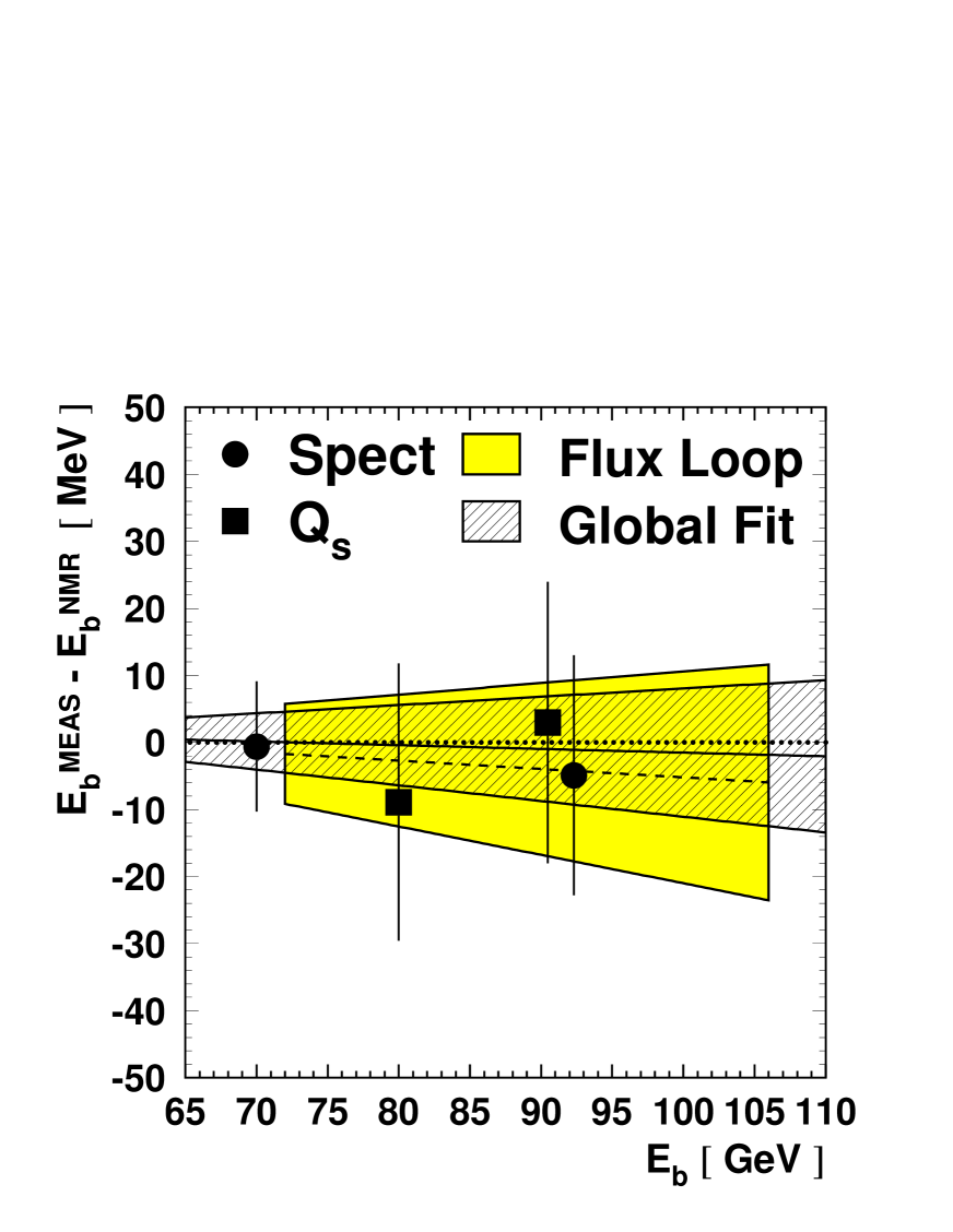
Figure 45: The difference between the measurements of $E_{\mathrm{b}}$ and the NMR model prediction, together with the results of the two-parameter fit. In the fit, the $Q_{s}$ data consist of five measurements at $E_{\mathrm{b}}$ = 80 GeV and one more precise measurement at $E_{\mathrm{b}}$ = 90 GeV. The 80 GeV measurements have been combined into a single point in this figure. Measurements made with the same method have correlations which are discussed in the text.

The fit has been repeated with various subsets of the input data. These include the flux-loop and spectrometer alone; the flux-loop and $Q_{s}$ alone; the spectrometer and $Q_{s}$ alone; the standard set without the contribution of the single 90 GeV $Q_{s}$ measurement; and the standard set without the 70 GeV spectrometer input. The results and errors, at three illustrative running points, are shown in table 23, together with the results of the standard fit and the results of the flux-loop analysis. It can be seen that the three methods have comparable weight and produce similar results. The combined measurements of the spectrometer and $Q_{s}$ provide a more precise result than the more indirect method of the flux-loop. The $Q_{s}$ data have significant weight in the fit even when the single most precise measurement at 90 GeV is excluded. Dropping the 70 GeV spectrometer fit point from the combination leads to a very small degradation in precision. In all cases the results support the mean NMR-model over the full range of energies.

	Offset	Slope	Error [MeV] at $E_{\mathrm{CM}}^{\mathrm{nom}}$ of:
Variant	[MeV]	[MeV/GeV]	161 GeV	200 GeV	207 GeV
FL, Spect and $Q_{s}$	-1.5	-0.06	6.1	9.5	10.2
FL and Spect	-5.1	-0.12	8.0	12.4	13.3
FL and $Q_{s}$	-0.1	-0.03	6.9	10.8	11.5
Spect and $Q_{s}$	-0.9	-0.02	11.2	14.5	15.1
FL alone	-5.2	-0.13	10.1	15.7	16.8
No 90 GeV $Q_{s}$	-1.8	-0.06	6.4	10.0	10.7
No 70 GeV Spect	-1.7	-0.06	6.2	9.6	10.2

Table 23: Fitted offset at 100 GeV and slope with energy, and errors on the offset at three illustrative LEP 2 energy points, for various sub-sets of input data. Also shown are the input measurements for the flux-loop alone. (Note that the errors have been evaluated at the luminosity weighted energies calculated by the model, rather than the $E_{\mathrm{CM}}^{\mathrm{nom}}$ values displayed.)

To go from the errors on the results of the mean NMR-model to those appropriate for each energy point an uncertainty of 2 MeV is added, in common between the energy points of 1999, otherwise uncorrelated, to allow for year-to-year variation in the model from changing calibration coefficients. The value of this component is once more motivated by the typical size of entries in the bottom row of table 3.

It is known that the change in calibration is much larger between 1996 and the later years, and so the exact results of the mean model fit are not applicable to the earlier dataset. Nevertheless, the fit demonstrates clearly that the magnetic model procedure is not subject to any significant non-linearity. Therefore, for the two 1996 energy points additional contributions of 9.6 MeV and 10.3 MeV are added to the mean model errors, these being the statistical uncertainties on the individual model for this year. The values are derived from the observed RMS scatters of the 16 individual values of $E_{\mathrm{b}}^{\mathrm{MOD}\,i}$ in expression 6, at collision energies of 161 and 172 GeV respectively.

The errors on $E_{\mathrm{CM}}^{\mathrm{MOD}}$ associated with the NMR model for each energy point of LEP 2 are presented in the first row of entries in table 24. These are twice those values calculated for $E_{\mathrm{b}}$.

11 Summary of Results and Systematic Uncertainties

11.1 High-Energy Analysis

The results from the combination of the NMR tests as presented in table 22 are corrections which must be applied to the output, $E_{\mathrm{CM}}^{\mathrm{MOD}}$, of the energy model. The errors on these corrected values come from considering the errors from the NMR model, including year-to-year variation, the additional model uncertainties discussed in sections 4 and 5, and the small uncertainty arising from the RDP measurement itself. These errors are given in table 24 for each nominal energy point. The dominant component for all years is the NMR model error, apart from in 2000 where the BFS uncertainty is more important. The next largest contribution comes from the error on the RF sawtooth, which is 8–10 MeV. Table 25 shows the accompanying correlation matrix. For almost all energy points taken after 1996 the correlation is close to 100%. The correlation between the 2000 errors and those of the earlier years is less because of the BFS.

$E_{\mathrm{CM}}^{\mathrm{nom}}$  [GeV]	161	172	183	189	192	196	200	202	205	207
NMR model	22.8	25.0	16.5	17.6	18.1	18.8	19.5	19.8	20.4	20.7
RDP	1.0	1.0	1.0	1.0	1.0	1.0	1.0	1.0	1.0	1.0
$f^{\mathrm{RF}}_{c}$	0.0	0.0	5.4	5.6	5.8	5.8	6.0	6.0	0.0	0.0
$\alpha_{c}$	0.3	0.4	3.5	4.4	4.4	5.2	4.7	3.0	2.3	1.4
$\Delta E_{\mathrm{b}}$ in fill	1.0	1.0	1.0	1.0	1.0	1.0	1.0	1.0	1.0	1.0
Hcor/BFS	1.6	1.8	3.4	4.6	0.6	1.0	0.2	0.6	28.6	34.4
QFQD	1.4	1.4	0.6	0.6	0.6	0.8	0.8	0.8	0.8	0.8
RF sawtooth	10.0	10.0	8.0	8.0	8.0	10.0	10.0	10.0	10.0	10.0
$e^{+}e^{-}$ difference	4.0	4.0	4.0	4.0	4.0	4.0	4.0	4.0	4.0	4.0
Dispersion	2.0	2.0	2.0	2.0	2.0	2.0	2.0	2.0	2.0	2.0
Total	25.4	27.4	20.3	21.6	21.6	23.2	23.7	23.7	36.9	41.7

Table 24: Summary of systematic errors on $E_{\mathrm{CM}}^{\mathrm{MOD}}$, in MeV, at all nominal energy points.

$E_{\mathrm{CM}}^{\mathrm{nom}}$  [GeV]	161	172	183	189	192	196	200	202	205	207
161	1.00	1.00	0.57	0.56	0.57	0.57	0.58	0.58	0.38	0.34
172	1.00	1.00	0.58	0.57	0.58	0.59	0.59	0.59	0.39	0.35
183	0.57	0.58	1.00	0.94	0.95	0.95	0.95	0.94	0.57	0.51
189	0.56	0.57	0.94	1.00	0.94	0.94	0.94	0.93	0.57	0.50
192	0.57	0.58	0.95	0.94	1.00	1.00	1.00	0.99	0.58	0.52
196	0.57	0.59	0.95	0.94	1.00	1.00	1.00	0.99	0.58	0.52
200	0.58	0.59	0.95	0.94	1.00	1.00	1.00	1.00	0.59	0.52
202	0.58	0.59	0.94	0.93	0.99	0.99	1.00	1.00	0.59	0.53
205	0.38	0.39	0.57	0.57	0.58	0.58	0.59	0.59	1.00	0.99
207	0.34	0.35	0.51	0.50	0.52	0.52	0.52	0.53	0.99	1.00

Table 25: Correlation matrix for errors on $E_{\mathrm{CM}}^{\mathrm{MOD}}$ at all nominal energy points.

11.2 Uncertainty for ${\mathrm{Z}}$ Runs and Lower-Energy Data

The energy model has been used to calculate collision energies for the fills at the ${\mathrm{Z}}$ resonance, scheduled for the purposes of providing calibration data for the experiments. As the energy scale of ${\mathrm{Z}}$ running is directly set by RDP, the NMR model is no longer a source of uncertainty. Most other error sources are also smaller at these energies. An upper bound of 10 MeV can be assigned as the total error on $E_{\mathrm{CM}}^{\mathrm{MOD}}$ for ${\mathrm{Z}}$ operation during the LEP 2 programme.

The uncertainty on $E_{\mathrm{CM}}^{\mathrm{MOD}}$ for the 130-136 GeV running in 1997 is conservatively assumed to be the same as for the higher-energy operation in that year, and so it is set to 20 MeV.

12 Centre-of-mass Energy Spread

The spread in centre-of-mass energy is relevant for evaluating the width of the W boson, which is about 2 GeV and is measured with the full LEP 2 dataset with a statistical precision of around 70 MeV [1]. The spread of the beam energy, $\sigma_{E_{\mathrm{b}}}$, varies as $E_{\mathrm{b}}^{2}$, with an optics-dependent correction associated with any RF frequency shift. The value of the spread has been calculated to accompany each energy record distributed to the experiments. In order to obtain the centre-of-mass energy spread, $\sigma_{E_{\mathrm{CM}}}$, it is necessary to multiply $\sigma_{E_{\mathrm{b}}}$ by $\sqrt{2}$. The luminosity-weighted values of $\sigma_{E_{\mathrm{CM}}}$ are shown in table 26 for each nominal energy point. The decrease in $\sigma_{E_{\mathrm{CM}}}$ seen for 202 GeV and above is because of the smaller frequency shifts applied at these running points.

$E_{\mathrm{CM}}^{\mathrm{nom}}$ [GeV]	$\sigma_{E_{\mathrm{CM}}}$ [MeV]
161	$144\pm 7$
172	$165\pm 8$
183	$218\pm 11$
189	$236\pm 12$
192	$255\pm 13$
196	$265\pm 13$
200	$264\pm 13$
202	$250\pm 12$
205	$236\pm 24$
207	$235\pm 24$

Table 26: Luminosity-weighted centre-of-mass energy spreads, $\sigma_{E_{\mathrm{CM}}}$.

Measurements of the longitudinal bunch length at an interaction point, performed with the 1996 and 1997 data, have been used in conjunction with the measured values of $Q_{s}$ to make indirect determinations of $\sigma_{E_{\mathrm{b}}}$, as reported in [2]. These results agree well with the calculated values given to the experiments.

The error on the calculated energy spread in 1996–1999 is estimated to be about $5\%$, fully correlated between years. This value is assigned from the differences observed with respect to the result of the analytic calculation, when a simulation of the photon emission process is implemented. The error is 10% in 2000, because of additional uncertainties associated with the BFS. The corresponding uncertainty on the W width is negligible.

13 Conclusions

The method of energy determination, based on the NMR magnetic model calibrated through resonant depolarisation, has enabled the collision energies to be calculated for all LEP 2 running. Three independent methods have been used to verify the linearity of this calibration at high energy. Uncertainties on other ingredients in the energy model have been assigned, benefitting from the detailed understanding acquired during the LEP 1 Z resonanace scans, and from subsequent measurements. The total uncertainty for each energy point is presented in table 24, and the corresponding correlation matrix is given in table 25. For the majority of the data, collected in the 1997-1999 runs, the relative uncertainty is $1.1-1.2\times 10^{-4}$. For the operation in 2000 this error rises to $2.0\times 10^{-4}$ at the highest energies. This increase is driven by the uncertainty associated with the spreading of the bending field applied in order to raise the maximum beam energy.

The error induced on $M_{\mathrm{W}}$ from the collision energy uncertainty depends on the point-to-point correlations, the relative statistical uncertainties at these points, and the correlations in the other systematic errors contributing to $M_{\mathrm{W}}$. With the presently available preliminary results [1] the error on $M_{\mathrm{W}}$ from the collision energy is determined to be around 10 MeV/$c^{\mathrm{2}}$ [29]. This contribution is small compared with the statistical uncertainty on the $M_{\mathrm{W}}$ measurement.

References

- [1] The LEP Collaborations and the LEP W Working Group, Combined Preliminary Results on the Mass and Width of the W Boson Measured by the LEP Experiments, LEPEWWG/MASS/2003-01, ALEPH 2003-007 PHYSIC 2003-004, DELPHI 2003-007-CONF-629, L3 Note 2794, OPAL TN-734, March 2003.
- [2] A. Blondel et al. (LEP Energy Working Group), Eur. Phys. J. C. C11 (1999) 573.
- [3] R. Assmann et al. (LEP Energy Working Group), Eur. Phys. J. C6 (1999) 187.
- [4] See for example: P. Janot, What are the Priorities for LEP in its Final Year and M. Lamont, Strategies for Maximising Energy and Luminosity in ‘Proceedings of the Workshop on LEP-SPS Performance - Chamonix X’, CERN-SL-2000-07 DI.
- [5] A.A. Sokolov and I.M. Ternov, Sov. Phys. Dokl. 8 (1964) 1203.
- [6] L. Arnaudon et al., Phys. Lett. B284 (1992) 431; L. Arnaudon et al., Z. Phys. C66 (1995) 45.
- [7] B. Dehning et al., Dynamic Beam Based Calibration of Beam Position Monitors, EPAC 1998, Stockholm, Sweden, IoP publishing, 430.
- [8] J. Uythoven, A LEP (60,60) Optics for Energy Calibration Measurements, CERN-SL-97-58 OP.
- [9] J. Wenninger, Orbit Steering and Central Frequency for LEP 2 Energy Calibration, CERN-SL-2000-09 OP.
- [10] J. Wenninger, Radial Deformations of the LEP Ring, CERN-SL-95-21 OP.
- [11] P. Melchior, Tidal Interactions in the Earth Moon System, Communications, Serie B, No. 160 IUG General Assembly, Vienna, August 1991. Computer code courtesy of P. Melchior, Observatoire Royal de Belgique.
- [12] J. Wenninger, Measurement of Tidal Deformation of the LEP Ring with Closed Orbits, CERN-SL-96-22 OP.
- [13] J. Wenninger, Orbit Corrector Magnets and Beam Energy, CERN-SL-97-06 OP.
- [14] A. Beuret et al., Proposal to Increase the LEP Energy with Horizontal Orbit Correctors, CERN-SL-2000-014 MS.
- [15] J. Wenninger, RF System Calibration Using Beam Orbits at LEP, CERN-SL-2002-28 OP, LEP Energy Working Group 02/01.
- [16] M.D. Hildreth, A Systematic Check of SC Cavity Alignment Using LEP Beams, LEP Energy Working Group 97-03.
- [17] J. Billan et al., Magnetic Performance of the LEP Bending Magnets, PAC 1989, Chicago, USA, IEEE (1989) 1148.
- [18] L. Arnaudon et al. (LEP Energy Working Group), The Energy Calibration of LEP in 1991, CERN-PPE/92-125.
- [19] F. Roncarolo, The LEP Spectrometer Project: High Accuracy Magnetic Field Mapping of the Spectrometer Magnet, Tesi di Laurea in Ing. Nucleare (2000), Politecino di Milano; F. Roncarolo et al., The LEP Spectrometer Dipole Re-Mapping, IMMW 2001, Grenoble, France, http://www.esrf.fr/conferences/proceedings/IMMW12/ .
- [20] See for example: J.A. Hinkson and K.B. Unswer, Precision Analog Signal Processor for Beam Position Measurements in Electron Storage Rings, DIPAC 1995, Lubeck-Travemunde, Germany, published in DESY M-95 07, 124; K.B. Unswer, New Generation Electronics Applied to Beam Position Monitors, BIW 1996, Argonne, USA, A.I.P. Conference Proceedings 390 (1997) 527.
- [21] E. Barbero et al., Performance of BPM Electronics for the LEP Spectrometer, BIW 2000, Cambridge, Massachusets, USA, A.I.P. Conference Proceedings 546 (2000) 493.
- [22] J. Matheson, Nucl. Inst. and Meth. A466 (2001) 436.
- [23] J. Prochnow, The LEP Energy Spectrometer, Diploma thesis (2000) Fakultät für Mathematik, Informatik und Naturwissenschaften der Rheinisch-Westfälischen Technischen Hochschule Aachen.
- [24] H. Grote and F. C. Iselin, The MAD program, CERN-SL-90-13 AP (Rev. 4, 1995).
- [25] See for example: H. Wiedemann, Particle Accelerator Physics, volume I, Springer-Verlag (1993), chapters 8 and 9.
- [26] See for example: H. Wiedemann, Particle Accelerator Physics, volume II, Springer-Verlag (1995), chapter 10.
- [27] See for example: A. Chao and M. Tigner (editors), Handbook of Accelerator Physics and Engineering, World Scientific (1998) 209.
- [28] K. Hanke, private communication.
- [29] C.J. Parkes on behalf of the LEP W Working Group, private communication.