Abstract

If no light Higgs boson exists, the interaction among the gauge bosons becomes strong at high energies ($\sim 1\,{\rm TeV}$). The effects of strong electroweak symmetry breaking (SEWSB) could manifest themselves indirectly as anomalous couplings before they give rise to new physical states like resonances. Here a study of the measurement of trilinear gauge couplings is presented looking at the hadronic decay channel of the W boson at an $e\gamma$ - collider. A sensitivity in the range of $10^{-3}$ to $10^{-4}$ can be reached depending on the coupling under consideration.

1 Introduction

The measurement of trilinear gauge couplings (TGCs) at a photon collider (PC) [1] gives the possibility to study the bosonic sector of the Standard Model (SM). Due to the non-Abelian nature of the gauge group which describes the electroweak interactions, it is predicted that the gauge bosons interact among themselves, giving rise to vertices with three or four gauge bosons. Each vertex is described by dimensionless couplings, denoted as TGCs or QGCs (triple or quartic gauge couplings) with a strength obtained in the SM applying the ${SU(2)_{L}}\times{U(1)_{Y}}$ gauge symmetry. Possible deviations from the values predicted by the SM, that could occur at high energies ($\sim 1\,{\rm TeV}$), may indicate a signal of New Physics (NP) beyond the SM. In this case the SM can be considered as a lower energy approximation of another larger theory. The effects of this larger theory are contained in a Lagrangian expanded in power of $\frac{1}{\Lambda_{NP}}$, where $\Lambda_{NP}$ is the scale of the NP:

$${\cal L}_{eff}=\sum_{n\geq 0}\sum_{i}\frac{\alpha_{i}^{n}}{{\Lambda_{NP}}^{n}}{O}_{i}^{(n+4)}$$

where the coefficients ${\alpha}_{i}$ are obtained from the parameters of the high energy theory and parametrise all possible effects at low energy. The low-energy effective Lagrangian without a Higgs violates unitarity at a scale of 4$\pi\upsilon\approx 3\,{\rm TeV}$, so that new physics should appear below this scale.

Conventionally the trilinear gauge boson vertices, involving only W and $\gamma$ bosons, are parametrised by the most general effective Lagrangian as [2]:

$${\cal L}_{TGC}^{WW} = -ie\left[g_{1}^{\gamma}V^{\mu}(W_{\mu\nu}^{-}W^{+\nu}-W_{\mu\nu}^{+}W^{-\nu})+{\kappa}_{\gamma}W_{\mu}^{+}W_{\nu}^{-}V^{\mu\nu}\right.$$

$$+\frac{{\lambda}_{\gamma}}{M_{W}^{2}}V^{\mu\nu}W_{\nu}^{+\rho}W_{\mu\rho}^{-}$$

$$+i{g_{5}^{\gamma}}{\varepsilon_{\mu\nu\rho\sigma}}[({\partial}^{\rho}W^{-\mu})W^{+\nu}-{W^{-\mu}}({\partial}^{\rho}W^{+\nu})]V^{\sigma}$$

$$+ig_{4}^{\gamma}W_{\mu}^{-}W_{\nu}^{+}({\partial}^{\mu}V^{\nu}-{\partial}^{\nu}V^{\mu})$$

$$\left.-\frac{\tilde{{\kappa}_{\gamma}}}{2}W_{\mu}^{-}W_{\nu}^{+}{\varepsilon}^{\mu\nu\rho\sigma}V^{\rho\sigma}-\frac{\tilde{{\lambda}_{\gamma}}}{2M_{W}^{2}}W_{\rho\mu}^{-}W_{\nu}^{+}{\varepsilon}^{\nu\rho\alpha\beta}V_{\alpha\beta}]\right],$$

where $M_{W}$ is the nominal $W^{\pm}$ mass, $V$ is the photon field, $W^{\pm}$ are the W fields, and the field tensors are given as $W_{\mu\nu}={\partial}^{\mu}W^{\nu}-{\partial}^{\nu}W^{\mu}$ and $V_{\mu\nu}={\partial}^{\mu}V^{\nu}-{\partial}^{\nu}V^{\mu}$. $\varepsilon^{\alpha\beta\gamma\delta}$ is the fully antisymmetric $\varepsilon$-tensor. The seven coupling parameters of $\gamma$WW vertices are grouped according to their symmetries as C and P conserving couplings ($g_{1}^{\gamma},{\kappa}_{\gamma}$ and ${\lambda}_{\gamma}$), C,P violating but CP conserving couplings ($g_{5}^{\gamma}$) and CP violating couplings ($g_{4}^{\gamma},{\tilde{{\kappa}_{\gamma}}}$ and ${\tilde{{\lambda}_{\gamma}}}$). In the SM all couplings are zero except $g_{1}^{\gamma}=1$ and ${\kappa}_{\gamma}=1$. As it was already mentioned, deviations from the SM prediction, denoted as ${\Delta}{\kappa}_{\gamma}(={\kappa}_{\gamma}-1)$ and ${\lambda}_{\gamma}$, arise as a consequence of a new physics effect. Introducing deviations of coupling parameters (“anomalous couplings”) from those given in the SM, the previous Lagrangian in general describes non-renormalisable and unitarity violating interactions. This analysis studies the measurement of the C and P conserving couplings, ${\kappa}_{\gamma}$ and ${\lambda}_{\gamma}$, while the value of $g_{1}^{\gamma}$ is fixed by electro-magnetic gauge invariance ($g_{1}^{\gamma}=1$). The other couplings are assumed to vanish.

The low energy effective Lagrangian for triple gauge boson vertices, in non-linear realisation of the symmetry can be expressed in terms of the two operators, ${\cal L}_{9L}$ and ${\cal L}_{9R}$ [3], where

$${\cal L}_{9L} = ig_{W}\frac{L_{9L}}{{16\pi}^{2}}Tr[W^{\mu\nu}D_{\mu}\Sigma D_{\nu}\Sigma^{+}],$$

$${\cal L}_{9R} = ig_{W}^{{}^{\prime}}\frac{L_{9R}}{{16\pi}^{2}}Tr[B^{\mu\nu}D_{\mu}\Sigma D_{\nu}\Sigma^{+}].$$

${L}_{9L}$ and ${L}_{9R}$ are parameters expected to be of ${\cal O}(1)$ while $D_{\mu}\Sigma$ represents the ${SU(2)}\times{U(1)}$ covariant derivative and $\Sigma=\exp(i{\vec{\omega}}\cdot{\vec{\sigma}}/{\upsilon})$ describes the Goldstone bosons with the built-in custodial $SU(2)_{C}$ symmetry. Taking the physical fields instead the Goldstone bosons the following relation can be obtained:

$${\kappa}_{\gamma}=1+\frac{e^{2}}{{\sin^{2}\theta_{W}}}\frac{{1}}{{32\pi}^{2}}(L_{9L}+L_{9R}).$$

Taking the operators of higher dimension, ${\lambda}_{\gamma}$ is expected to be:

$${\lambda_{\gamma}}=(\frac{e^{2}}{{\sin^{2}\theta_{W}}})L_{\lambda}\frac{{M_{W}}^{2}}{{\Lambda_{NP}}^{2}}.$$

If one assumes that any deviation from the SM values is induced by scattering of Goldstone bosons at high energy scales associated with spontaneous symmetry breaking, this effective description without a physical Higgs boson could explain the mass generation via the mechanism of SEWSB.

2 Observables Sensitive to the Triple Gauge Couplings

We studied single W boson production in high energy $e\gamma$ collisions ($e^{-}\gamma\rightarrow W^{-}\nu_{e}$) and the sensitivity of some observables like angular distributions, to the $\gamma$WW gauge boson couplings. In $e\gamma$ collisions the TGCs contribute only through t-channel W-exchange at the ${\gamma}$WW vertex as it is shown in Fig. 1 b. The beam electrons have to be left-handed since the W boson does not couple to right-handed electrons. On the other hand, the photons can be right-handed or left-handed. The differential cross-section for the two different initial photon helicities is shown in Fig. 1 a. For left-handed photons the s-channel contribution leads to a higher differential cross-section. The contribution of each W helicity state to the total cross-section for different centre-of-mass energies is shown in Fig. 2. The contribution of each W helicity state to the differential cross-section is shown in Fig. 3.

Figure 1: Left (a): SM differential cross-section distributions for two different initial photon helicities - left-handed (red line-upper) and right-handed (blue line-lower) at $\sqrt{s_{e\gamma}}=450\,{\rm GeV}$. The contribution from the s-channel is visible for left-handed photons leading to a larger cross-section. Right (b): Feynman diagrams contributing to $e^{-}\gamma\rightarrow W^{-}\nu_{e}$ with TGC contribution only through t-channel W-exchange.

Figure 2: Total lowest-order cross-sections as a function of ${\sqrt{s_{e\gamma}}}$ for different boson polarisations assuming that the electron is left-handed. Left: without an angular cut. Right: with an angular cut $20^{\circ}\leq\theta\leq 160^{\circ}$. Notation: ($h_{\gamma},h_{W}$) = ($\gamma$ helicity, W helicity).

For the boson polarisations $(h_{\gamma},h_{W})=(-1,+1)$ and $(-1,0)$ the SM amplitudes are equal to zero. Different W-helicity states are contained in the differential cross-section distribution over the decay angle:

$${\frac{{d^{2}\sigma}}{d\cos\theta d\cos{\theta}_{1}}}={\frac{3}{4}}\left[{\frac{1}{2}}{\frac{{d{\sigma}_{T}}}{d\cos\theta}}(1+{\cos^{2}}{\theta_{1}})+{\frac{{d{\sigma}_{L}}}{d\cos\theta}}{\sin^{2}}{\theta_{1}}\right],$$

where $\theta$ denotes the production angle of the W and $\theta_{1}$ denotes the decay angle. ${\frac{{d{\sigma}_{T}}}{d{\cos\theta}}}$ is the differential cross section for the production of transversally polarised W-bosons distributed as ${(1+{\cos^{2}}{\theta_{1}})}$ and ${\frac{{d{\sigma}_{L}}}{d{\cos\theta}}}$ is the differential cross section for longitudinal W production, distributed as ${\sin^{2}}{\theta_{1}}$.

Figure 3: Contribution of each W helicity state for two different initial photon polarisations to the SM differential cross-section at $\sqrt{s_{e\gamma}}=450\,{\rm GeV}$. The angle $\theta$ is defined as the angle between the $\gamma$ beam and the outgoing W. Notation: ($h_{\gamma},h_{W}$) = ($\gamma$ helicity, W helicity).

Anomalous TGCs affect both the total production cross-section and the shape of the differential cross-section as a function of the W production angle. As a consequence, distributions of W decay products are changed also. The relative contribution of each helicity state of the W boson to the total cross-section in the presence of anomalous couplings is shown in Fig. 4. Fig. 5 a shows that the differential cross-section distribution in the backward region is more sensitive to the presence of anomalous TGC in the case of right-handed photons than for left-handed ones. Fig. 5 b shows the $W_{L}$ fraction if there are anomalous couplings and in the SM. The production of $W_{L}$ bosons in the presence of anomalous couplings will differ from the SM. This behaviour comes from the fact that the information about SEWSB can be obtained through the study of Goldstone boson interactions which are the longitudinal component of the gauge bosons. Differential cross-sections are calculated on the basis of the formula given in [4] using helicity amplitudes in the presence of anomalous couplings from [5]. In W production via $e\gamma$ collisions the favourable initial $\gamma$-$e$ helicity states are “right-left” respectively. Because of the missing s-channel electron-exchange in this state, the W boson angular distributions show larger sensitivity to TGCs in the backward region than in the case with initial left-handed photons.

Figure 4: Contribution of different W helicity states for two different initial photon polarisations in the presence of anomalous couplings, ${\Delta}{\kappa}_{\gamma}$ (left plot) and ${\lambda}_{\gamma}$ (right plot) at $\sqrt{s_{e\gamma}}=450\,{\rm GeV}$. Notation: ($h_{\gamma},h_{W}$) = ($\gamma$ helicity, W helicity).

Figure 5: Left (a): Differential cross-section in the presence of anomalous TGCs for both initial photon helicity states - left-handed (blue-outer lines) and right-handed (red-inner lines), normalised to their SM values at $\sqrt{s_{e\gamma}}=450\,{\rm GeV}$. Right (b): Deviation of longitudinal W fraction in presence of anomalous TGCs from the SM for ${\Delta}{\kappa}_{\gamma}={\pm}0.01$ at $\sqrt{s_{e\gamma}}=450\,{\rm GeV}$.

3 Signal and Background Simulation

The energetic, highly polarised photons can be produced at a high rate in Compton backscattering of laser photons on high energy electrons [1]. Setting opposite helicities for the laser photons and the beam electrons the energy spectrum of the backscattered photons is peaked at $\sim 80\,{\%}$ of the electron beam-energy. The backscattered photons are highly polarised in this high energy region. With an integrated luminosity in the real mode of $71\,{\rm fb}^{-1}/{\rm year}$ for $\sqrt{s_{e\gamma}}>0.8\sqrt{s_{e\gamma}({\rm max})}$ [1], $3\cdot 10^{6}$ Ws per year can be produced in $e^{-}\gamma\rightarrow W^{-}\nu_{e}$ with hadronically decaying Ws, assuming $100\,{\%}$ detector acceptance. In the parasitic mode the luminosity is even slightly higher.

A photon collider can operate as a $\gamma\gamma$- or as an $e\gamma$-collider. $e\gamma$-collisions can be studied in two different modes - the real and the parasitic one. In the real mode electrons from only one electron beam are converted into high energy photons ($e\gamma$-collider). If the electrons from both electron beams are converted into high energy photons the $\gamma\gamma$-collider is realised and the interactions between backscattered photons and unconverted electrons from both sides can be used in the parasitic $e\gamma$ mode.

The beam spectra for the different collider modes at ${\sqrt{s_{ee}}=500}\,{\rm GeV}$ are simulated using CIRCE2 [6]. CIRCE2 is a fast parameterisation of the spectra described in [1] including multiple interactions and non-linearity effects. The used spectra for the two modes are shown in Fig. 6.

Figure 6: $e\gamma$ luminosity spectra for the real (left) and parasitic (right) mode simulated with CIRCE2 for ${\sqrt{s_{ee}}=500}\,{\rm GeV}$.

The response of the detector has been simulated with SIMDET V4 [7], a parametric Monte Carlo for the TESLA $e^{+}e^{-}$ detector. It includes a tracking and calorimeter simulation and a reconstruction of energy-flow-objects (EFO). Only the EFOs with a polar angle above $7^{\circ}$ are taken for the W boson reconstruction simulating the acceptance of the PC detector as the only difference to the $e^{+}e^{-}$ detector [8]. W bosons are reconstructed using the hadronic decay channel (BR=0.68). The signal and background events are studied on a sample of events generated with WHIZARD [9].

The hadronic cross-section for ${\gamma\gamma}{\rightarrow}{\rm hadrons}$ events, within the energy range above $2\,{\rm GeV}$, is several hundred nb [10] so that ${\cal O}(1)$ events of this type are produced per bunch crossing (pileup). These events are overlayed to the signal events. Depending on the photon spectra the hadronic cross-section and the number of hadronic events can be calculated using different models including real and virtual photons [11]. Since these events are induced by t-channel q-exchange most of the resulting final state particles are distributed at low angles.

The informations about the neutral particles (neutrals) from the calorimeter and charged tracks (tracks) from the tracking detector are used to reconstruct the signal and background events. The considered backgrounds depend on the two different modes of the $e\gamma$-collider and for both modes result in a ${q}{\bar{q}}$-pair in the final state. Due to the different $\gamma\gamma$ luminosities in the two $e\gamma$ modes, the pileup contribution to each mode is different - 1.2 events/BX for the real mode and 1.8 events/BX for the parasitic mode [12]. A large cross-section for W boson production (${\sigma}_{pol}\sim 45\,{\rm pb}$ for the hadronic channel) provides an efficient separation of signal from background applying several successive cuts.

For the real mode the considered backgrounds are following:

1. ${e}{\gamma}{\rightarrow}{e}{Z}{\rightarrow}e{q}{\bar{q}}$, where the events are simulated with a kinematic cut which allows only production of electrons at low angles (below $15^{\circ}$). The preselection cut used to reduce the background contributing to this channel was to reject events with a high energetic electron ($\geq 100\,{\rm GeV}$) in the detector. By this cut $33\%$ of the background events are rejected not affecting the signal efficiency.

2. ${\gamma}(e^{-}){\gamma}{\rightarrow}{q}{\bar{q}}$, simulating the interaction between a real, high energy photon and a virtual bremsstrahlung photon.

Additional backgrounds considered for the parasitic mode are the following:

1. ${\gamma}{\gamma}{\rightarrow}{W}{W}$, where one W decays leptonically and the other W decays hadronically. To reduce the background contributing from this channel in each event we searched for a lepton in the detector with an energy higher than $5\,{\rm GeV}$. For these leptons a cone of $30^{\circ}$ is defined around their flight directions and the energies of all particles (excluding the lepton) are summed inside the cone. Events with energies smaller than $20\,{\rm GeV}$ were rejected. This cut rejects $\sim 70\%$ of the semileptonic WW background events, not affecting the signal efficiency.

2. ${\gamma}{\gamma}{\rightarrow}{q}{\bar{q}}$, simulating the interaction between two real photons.

3.1 Energy flow and Event Selection

In order to minimise the pileup contribution to the high energy signal tracks the first step in the separation procedure was to reject pileup tracks as much as possible. The measurement of the impact parameter of a particle along the beam axis with respect to the primary vertex is used for this purpose. The beamspot length of 300$\mu{\rm m}$ for TESLA is simulated and shown in Fig. 7 a, representing the primary vertex distribution of events along the z-axis.

Figure 7: Left (a): Primary vertex distribution along the beam axis (blue - hatched) compared to the deviation of the reconstructed primary vertices for signal without (yellow-light) and with pileup (red-dark) tracks. Right (b): Separation efficiency for signal (blue-1) and pileup (red-2) tracks for $\textit{$I_{X,Y}$}\leq{2\sigma}$.

Using the precise measurements from the vertex detector first the primary vertex of an event is reconstructed as the momentum weighted average z-impact parameter, $I_{Z}$ of all tracks in the event. All impact parameters are then recalculated using this primary vertex. The reconstructed primary vertex distribution for signal with and without pileup tracks is also shown in Fig. 7 a. It can be seen that the distribution with pileup tracks is much broader than if there are only signal tracks. The separation efficiency for a cut on $|I_{Z}/\sigma|$ is shown in Fig. 7 b for tracks with a transversal impact parameter $I_{X,Y}$ less than ${2\sigma}$. If one selects the tracks with $I_{Z}$ less than ${2\sigma}$, about $\sim 60\,{\%}$ of the pileup tracks and only $\sim 5-10\,{\%}$ of the signal tracks are rejected. All tracks with $\textit{$I_{X,Y}$}\geq{2\sigma}$ are accepted since they could originate from a secondary vertex of a good track.

A reconstruction of the angle of each EFO with respect to the z-axis and the angle between the EFO and the flight direction of the reconstructed W (Fig. 8), makes it possible to distinguish further between signal and pileup EFOs. EFOs are rejected if they are positioned in the area shown in Fig. 8 b.

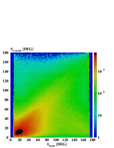
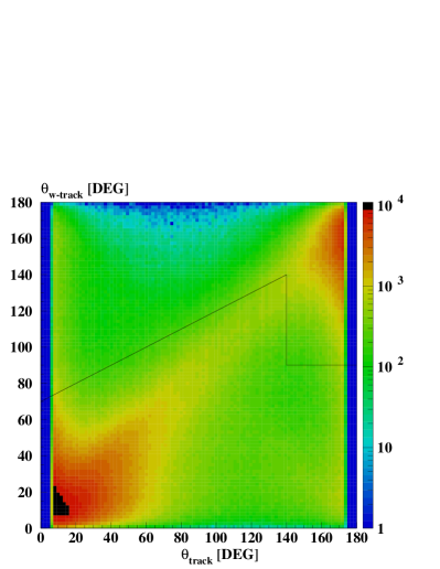
Figure 8: Angle of the energy flow objects with the beam axis versus their angle with the reconstructed W direction for signal only (left,a) and for signal plus pileup (right,b). The tracks above the line shown in b are rejected in the analysis.

The different steps during the separation procedure for the real and parasitic ${e}{\gamma}$-mode are shown in Fig. 9 and in Fig. 10. The shapes of the W distributions are restored, increasing the efficiency but getting worse resolutions.

Figure 9: Mass and energy distributions of the reconstructed W for the real mode during the different steps in the EFO rejection; initial shape (green-1), after the track rejection using $I_{Z}$ (red-2) and final shape (blue-3). Left (a): W mass distributions. Right (b): W energy distributions.

Figure 10: Same a Fig. 9 for the parasitic mode.

In order to separate the signal events from the background the events with a number of EFOs larger than 10 and a number of charged tracks larger than 5 are accepted only. We also applied in addition to the vetoes on high energy and isolated leptons cuts on two reconstructed variables, the energy ($100\,{\rm GeV}-250\,{\rm GeV}$) and the mass ($60\,{\rm GeV}-100\,{\rm GeV}$) of the reconstructed W boson. The final angular distributions of signal and background events for both ${e}{\gamma}$-modes are shown in Fig. 11.

Figure 11: Signal and background distributions for $e\gamma\rightarrow W\nu$ as a function of the W production angle. The different processes are normalised to the same luminosity. The blue (hatched) area represents the signal. Left (a): Real $e\gamma$ mode. The red (dark) contribution correspond to ${\gamma}(e^{-}){\gamma}{\rightarrow}{q}{\bar{q}}$ processes and the yellow one (light) correspond to $e\gamma\rightarrow eZ$. Right (b): Parasitic $e\gamma$ mode. The red (dark) contribution correspond to ${\gamma}{\gamma}{\rightarrow}{W}{W}$ while the yellow one (light) correspond to ${\gamma}{\gamma}{\rightarrow}{q}{\bar{q}}$ processes.

The efficiency obtained for the real mode is $73\,{\%}$ with a purity of $64\,{\%}$. In the parasitic mode, due to the fact that the pileup is larger than in the case of the real mode, the efficiency is $66\,{\%}$ with a purity is $49\,{\%}$. Background events are mostly distributed close to the beam pipe and an additional cut on the W production angle is applied in order to increase the purity of the signal in both modes. Events in the region below $5^{\circ}$ are rejected leading to a purity of $95\,{\%}$ for the real mode and $72\,{\%}$ for the parasitic mode. This cut has only a small influence on the signal resulting in efficiencies of $70\,{\%}$ and $63\,{\%}$ for real and parasitic mode, respectively.

4 Fit Method and Error Estimations

For the extraction of the triple gauge couplings from the reconstructed kinematical variables a ${\chi^{2}}$ fit is used. A sample of ${10^{6}}$ SM signal events is generated with WHIZARD and passed trough the detector simulation. The number of events obtained after the detector and after all cuts (Fig. 12) is normalised to the number of events we expect after one year of running of an $e\gamma$-collider.

Figure 12: Polar angle distributions of reconstructed Ws for the real (left) and parasitic (right) mode. The signal events are coloured with blue (hatched) while the red (full) distributions correspond to the background events.

Each event is described reconstructing three kinematical variables - the W production angle with respect to the ${e^{-}}$ beam direction, the W polar decay angle $\cos{\theta_{1}}$ (angle of the fermion with respect to the W flight direction measured in the W rest frame) and the azimuthal decay angle $\phi$ of the fermion with respect to a plane defined by W and the beam axis. The polar decay angle, $\cos{\theta_{1}}$ is sensitive to the different W helicity states and the azimuthal angle, $\phi$ to the interference between them. In hadronic W-decays the up- and down-type quarks cannot be separated so that only $|\cos\theta_{1}|$ is measured. The matrix element calculations from WHIZARD are used to obtain weights to reweight the angular distributions as functions of the anomalous TGCs. Each Monte Carlo SM event is weighted by a weight:

$${R({\Delta}{\kappa}_{\gamma},{\lambda}_{\gamma})=1+A{\Delta}{\kappa}_{\gamma}+B{{{\Delta}{\kappa}_{\gamma}}^{2}}+C{\lambda}_{\gamma}+D{{{\lambda}_{\gamma}}^{2}}+E{\Delta}{\kappa}_{\gamma}{\lambda}_{\gamma}}$$

where ${\Delta}{\kappa}_{\gamma}$ and ${\lambda}_{\gamma}$ are the free parameters. The function ${R({\Delta}{\kappa}_{\gamma},{\lambda}_{\gamma})}$ describes the quadratic dependence of the differential cross-section on the coupling parameters and it is obtained in the following way: using SM events (${\Delta}{\kappa}_{\gamma}={\lambda}_{\gamma}=0$) we recalculated the matrix elements of the events for a set of five different combinations of ${\Delta}{\kappa}_{\gamma}$ and ${\lambda}_{\gamma}$ values (Table 1).

	$R_{1}$	$R_{2}$	$R_{3}$	$R_{4}$	$R_{5}$
${\Delta}{\kappa}_{\gamma}$	0	0	+0.001	-0.001	+0.001
${\lambda}_{\gamma}$	+0.001	-0.001	0	0	+0.001

Table 1: ${\Delta}{\kappa}_{\gamma}$, ${\lambda}_{\gamma}$ values used to calculate the reweighting coefficients.

The resulting recalculated events carry a weight which is given by the ratio of the new matrix element values compared to the SM ones ($R_{i}$). The particle momenta are left unchanged. According to the chosen ${\Delta}{\kappa}_{\gamma},{\lambda}_{\gamma}$ combinations from Table 1 one gets:

$$R_{1} = 1+C\mid{\lambda}_{\gamma}\mid+D\mid{\lambda}_{\gamma}^{2}\mid,$$

$$R_{2} = 1-C\mid{\lambda}_{\gamma}\mid+D\mid{\lambda}_{\gamma}^{2}\mid,$$

$$R_{3} = 1+A\mid{\Delta}{\kappa}_{\gamma}\mid+B\mid{\Delta}{\kappa}_{\gamma}^{2}\mid,$$

$$R_{4} = 1-A\mid{\Delta}{\kappa}_{\gamma}\mid+B\mid{{{\Delta}{\kappa}_{\gamma}}^{2}\mid},$$

$$R_{5} = 1+A\mid{\Delta}{\kappa}_{\gamma}\mid+B\mid{{{\Delta}{\kappa}_{\gamma}}^{2}\mid}+C\mid{\lambda}_{\gamma}\mid+D\mid{{{\lambda}_{\gamma}}^{2}\mid}+E\mid{\Delta}{\kappa}_{\gamma}\mid\mid{\lambda}_{\gamma}\mid,$$

where $|{\Delta}{\kappa}_{\gamma}|$=$|{\lambda}_{\gamma}|$=0.001. The coefficients A,B,C,D,E are deduced for each event from the previous five equations. Four-dimensional ($\cos{\theta}$,$\cos{\theta_{1}},\phi$, energy) event distributions are fitted with MINUIT [13], minimizing the ${\chi^{2}}$ as a function of $\kappa_{\gamma}$ and $\lambda_{\gamma}$ taking the SM Monte Carlo sample as “data”:

$$\chi^{2}=\sum_{i,j,k,l}\frac{\left(z\cdot N^{SM}(i,j,k,l)-n\cdot z\cdot N^{{\kappa}_{\gamma},{\lambda}_{\gamma}}(i,j,k,l)\right)^{2}}{z\cdot\sigma^{2}(i,j,k,l)}+\frac{(n-1)^{2}}{(\Delta L^{2})}$$

where i, j and k run over the reconstructed angular distributions, l runs over the reconstructed W boson energy, $N^{SM}(i,j,k,l)$ are the “data” which correspond to the SM Monte Carlo sample, $N^{{\kappa}_{\gamma},{\lambda}_{\gamma}}(i,j,k,l)$ is the event distribution weighted by the function $R({\Delta}{\kappa}_{\gamma},{\lambda}_{\gamma})$ and $\sigma(i,j,k,l)=\sqrt{N^{SM}(i,j,k,l)}$. The factor ${z}$ sets the number of signal events to the expected one after one year of running of an $e\gamma$-collider. In case where the background is included in the fit ${z}$ defines the sum of signal and background events and ${n}\cdot N^{{\kappa}_{\gamma},{\lambda}_{\gamma}}\rightarrow[{n}\cdot N_{signal}^{{\kappa}_{\gamma},{\lambda}_{\gamma}}+N_{bck}]$. The number of background events is normalised to the effective W production cross-section in order to obtain the corresponding number of background events after one year of running of an $e\gamma$-collider. It is assumed that the total normalisation (efficiency, luminosity, electron polarisation) is only known with a relative uncertainty $\Delta L$. To do this $n$ is taken as a free parameter in the fit and constrained to unity with the assumed normalisation uncertainty. Per construction the fit is bias-free and thus returns always exactly the SM as central values.

Table 2 shows the estimated statistical errors we expect for the different couplings at ${\sqrt{s_{ee}}=500}\,{\rm GeV}$ for two-parameter four-dimensional (4D) fit at detector level, with and without pileup. In this estimation the cut of $5^{\circ}$ is not applied. Table 3 contains the statistical errors obtained together with background events applying the cut on the W production angle of $5^{\circ}$.

	without pileup			with pileup
${{\Delta}L}$	1$\%$	0.1$\%$	0	1$\%$	0.1$\%$	0
${\Delta}{\kappa}_{\gamma}{\cdot}10^{-3}$	3.4/4.0	1.0/1.0	0.5/0.5	3.5/4.5	1.0/1.0	0.5/0.5
${\Delta}{\lambda}_{\gamma}{\cdot}10^{-4}$	4.9/5.5	4.5/5.2	4.5/5.1	5.2/6.7	4.9/6.4	4.9/6.4

Table 2: Estimated statistical errors for ${\kappa}_{\gamma}$ and ${\lambda}_{\gamma}$ from the two-parameter 4D fit at detector level for the real/parasitic $e\gamma$ mode without and with pileup.

	pileup+background
${{\Delta}L}$	1$\%$	0.1$\%$	0
${\Delta}{\kappa}_{\gamma}{\cdot}10^{-3}$	3.6/4.8	1.0/1.1	0.5/0.6
${\Delta}{\lambda}_{\gamma}{\cdot}10^{-4}$	5.2/7.0	4.9/6.7	4.9/6.7

Table 3: Estimated statistical errors for ${\kappa}_{\gamma}$ and ${\lambda}_{\gamma}$ from the two-parameter 4D fit at detector level for the real/parasitic $e$$\gamma$ mode with pileup and background events.

The main error on ${\kappa}_{\gamma}$ comes from the luminosity measurement while ${\lambda}_{\gamma}$ is not sensitive to that uncertainty. The two different $e\gamma$ modes give the same estimation for ${\Delta}{\kappa}_{\gamma}$ while ${\Delta}{\lambda}_{\gamma}$ is more sensitive to the different modes. The difference in the estimated ${\Delta}{\lambda}_{\gamma}$ for two modes is a consequence of the ambiguity in the W production angle which is present in the parasitic mode and due to the fact that the distance between the conversion region and the interaction point is larger in the real mode than in the parasitic mode. A smaller distance between the conversion and the interaction region increases the luminosity at the price of a broader energy spectrum. That decreases the sensitivity of the ${\lambda}_{\gamma}$ measurement.

The pileup contribution is larger in the parasitic than in the real mode and therefore it influences the W distributions (energy and angular) more than in the real mode. This leads to a decrease in sensitivity for ${\lambda}_{\gamma}$ of $\sim 10\,{\%}$ in the real and of $\sim 25\,{\%}$ in the parasitic mode while the influence on ${\Delta}{\kappa}_{\gamma}$ is negligible. The influence of the background is not so stressed as it is for the pileup. In the real mode it is almost negligible while it contributes to the parasitic mode decreasing the sensitivity of ${\lambda}_{\gamma}$ by less than $5\,{\%}$. The contour plot in ${\Delta}{\kappa}_{\gamma}-{\lambda}_{\gamma}$ plane, shown in Fig. 13 is based on the results given in Table 3 assuming a normalisation error of 0.1${\%}$.

Figure 13: 95$\%$ CL and 1$\sigma$ contours in the ${\Delta}{\kappa}_{\gamma}-{\lambda}_{\gamma}$ plane obtained from the 4D fit for ${{\Delta}L}=0.1\%$.

The correlation between the fit parameters ${\Delta}{\kappa}_{\gamma}$ and ${\Delta}{\lambda}_{\gamma}$ is found to be negligible and it is shown in Table 4 while ${\Delta}{\kappa}_{\gamma}$ strongly depends on n.

	pileup+background
	${\Delta}{\kappa}_{\gamma}$	n	${\Delta}{\lambda}_{\gamma}$
${\Delta}{\kappa}_{\gamma}$	1.000	-0.857	0.122
n	-0.857	1.000	-0.094
${\Delta}{\lambda}_{\gamma}$	0.122	-0.094	1.000

Table 4: Correlation matrix for the two-parameter fit (${{\Delta}L}=0.1\%$).

4.1 Systematic Errors

Due to the large W production cross-sections and achievable luminosities at the PC the statistical errors are comparable with those estimated for the $e^{+}e^{-}$-collider [14] and the main source of error comes from the systematics. Some sources of systematic errors have been investigated, assuming ${{\Delta}L}=0.1\%$. It was found that the largest uncertainty in ${\kappa}_{\gamma}$ comes from uncertainties on the photon beam polarisations. Contrary to the $e^{+}e^{-}$ case the luminosity and polarisation measurements are not independent. The dominant polarisation state ($J_{z}=3/2$) can be measured accurately with $e\gamma\rightarrow e\gamma$ while the suppressed one ($J_{z}=1/2$) can only be measured with worse precision e.g. using $eZ\rightarrow eZ$ [15]. To estimate the uncertainty on the TGCs therefore the dominant $J_{z}=3/2$ part is kept constant while the $J_{z}=1/2$ part is changed by 10%, corresponding to a 1% polarisation uncertainty for ${\cal P}_{\gamma}=0.9$. This leads to a polarisation uncertainty of $0.005$ for $\kappa_{\gamma}$, corresponding to five times the statistical error while the uncertainty on $\lambda_{\gamma}$ is negligible. The photon polarisation thus needs to be known to 0.1$\%$ - 0.2$\%$ so that ${\kappa}_{\gamma}$ is not dominated by this systematic error.

In order to estimate the error coming from the W mass measurement we recalculated the data sample with ${M_{W}}$ decreased/increased by $50\,{\rm MeV}$ (the expected ${\Delta}{M_{W}}$ at LHC is $\sim 15$ MeV) reweighting the SM events. The nominal W mass used for Monte Carlo sample was $M_{W}=80.419\,{\rm GeV}$. As a result of the recalculation we get the ratios of matrix element values corresponding to the nominal W mass and the mass $M_{W}^{{}^{\prime}}=M_{W}\pm\Delta M_{W}$. The Monte Carlo sample (MC) is weighted by this ratio and fitted as fake data leaving the reference distributions unchanged. The resulting shift for TGCs is of the order of the statistical error for both coupling parameters for $\Delta M_{W}=50\,{\rm MeV}$ and thus negligible with an improved W-mass measurement.

At the PC the field of the laser wave at the conversion region is very strong and the high energy electron or photon can interact simultaneously with several laser photons. These are nonlinear QED effects that influence the Compton spectra of the scattered photons in such a way that increasing the nonlinearity $\xi^{2}$ [1] the Compton spectrum becomes broader and shifted to lower energies. To estimate the error that comes from this effect the laser power is decreased changing $\xi^{2}$ from 0.3 $\rightarrow$ 0.15, increasing the peak energy by 2.5%. The ratio of the two Compton spectra is used as a weight function to obtain the “data” sample from the MC events. The sample data obtained in that way are fitted leaving the reference distributions unchanged. It was found that the beam energy uncertainty influences the measurement of the coupling parameters only via the normalisation $n$, and the errors ${\Delta}{\kappa}_{\gamma}$ and ${\Delta}{\lambda}_{\gamma}$ are considered as negligible since the value of $n$ is accessible from the luminosity measurement.

The estimated systematic error for $\kappa_{\gamma}$ from background uncertainties is smaller than the statistical error if the background cross section is know to better than 3% in the real mode and 1% in the parasitic mode. For $\lambda_{\gamma}$ the background needs to be known only to 10% in the parasitic mode while there are practically no restrictions in the real mode.

5 Conclusions

A future high energy $e\gamma$ collider provides an excellent opportunity to measure the gauge couplings between a W-pair and a photon. These couplings can be obtained without ambiguities from quartic or ZWW couplings. The expected precision is $10^{-3}$ for $\kappa_{\gamma}$ and $10^{-4}$ for $\lambda_{\gamma}$. While $\kappa_{\gamma}$ can be measured somewhat better in $e^{+}e^{-}$ [14] the $e\gamma$ collider seems to be the best place for a $\lambda_{\gamma}$ measurement.

References

- [1] ECFA/DESY Photon Collider Working Group, B. Badelek et al., TESLA Technical Design Report, Part VI, Chapter 1: Photon collider at TESLA, hep-ex/0108012, DESY-01-011E.
- [2] K.J.F. Gaemers and G.J. Gounaris, Zeit. Phys. C1 (1979) 259.
-
[3]
M. Baillargeon, G. Belanger, F. Boudjema, Electroweak
Physics Issues at a High Energy Photon Collider, hep-ph/9405359;
K. Hagiwara et al., Nucl. Phys. B282 (1987) 253. - [4] A.Denner, A.Dittmaier, Nucl. Phys. B398 (1993) 236.
- [5] E.Yehudai, Phys. Rev. D44 (1991) 3434.
-
[6]
T. Ohl, Circe Version 2.0: Beam Spectra for Simulating Linear
Collider and Photon Collider Physics,
ftp://heplix.ikp.physik.tu-darmstadt.de/pub/ohl/circe2/doc/manual.pdf. - [7] M.Pohl, H.J.Schreiber, SIMDET-Version 4 A parametric Monte Carlo for a TESLA Detector, DESY 02-061, May 2002.
- [8] K. Mönig, A Photon Collider at TESLA, LC-DET-2004-014.
- [9] W. Kilian,WHIZARD 1.24 A generic Monte Carlo integration and event generation package for multi-particle processes, LC-TOOL 2001-039 (revised).
- [10] The Particle Data Group, K. Hagiwara et al, Phys. Rev. D66 (2002) 010001.
- [11] D. Schulte, Study of Electromagnetic and Hadronic Background in the Interaction Region of the TESLA Collider, Thesis, April 1997.
- [12] D. Schulte, private communication.
- [13] F.James, MINUIT Function Minimization and Error Analysis, Version 94.1, CERN Program Library Long Writeup D506.
- [14] W. Menges, A Study of Charged Current Triple Gauge Couplings at TESLA, LC-PHSM-2001-022.
- [15] A. V. Pak, D. V. Pavluchenko, S. S. Petrosyan, V. G. Serbo and V. I. Telnov, Nucl. Phys. Proc. Suppl. 126 (2004) 379 [arXiv:hep-ex/0301037].