[hep-ex/0410010] A Precise Measurement of the Tau Lifetime

CERN–EP/2003-070

21 July 2003

DELPHI Collaboration

Abstract

The tau lepton lifetime has been measured with the ${\mbox{\rm e}^{+}\mbox{\rm e}^{-}\rightarrow\tau^{+}\tau^{-}}$ events collected by the DELPHI detector at LEP in the years 1991-1995. Three different methods have been exploited, using both one-prong and three-prong $\tau$ decay channels. Two measurements have been made using events in which both taus decay to a single charged particle. Combining these measurements gave $\tau_{\tau}\mbox{(1 prong)}=291.8\pm 2.3_{stat}\pm 1.5_{sys}\mbox{ fs}$ . A third measurement using taus which decayed to three charged particles yielded $\tau_{\tau}\mbox{(3 prong)}=288.6\pm 2.4_{stat}\pm 1.3_{sys}\mbox{ fs}.$ These were combined with previous DELPHI results to measure the tau lifetime, using the full LEP1 data sample, to be $\tau_{\tau}=290.9\pm 1.4_{stat}\pm 1.0_{sys}\mbox{\ fs}$ .

(Eur. Phys. J. C36 (2004) 283-296)

1 Introduction

The tau lepton is a fundamental constituent of the Standard Model and its lifetime can be used to test the model’s predictions. In particular, lepton universality can be probed using the relationships

	$\displaystyle\tau_{\tau}$	$\displaystyle=$	$\displaystyle\tau_{\mu}\left(\frac{g_{\mu}}{g_{\tau}}\right)^{2}\left(\frac{{\rm m}_{\mu}}{{\rm m}_{\tau}}\right)^{5}\cdot\mbox{BR}\left(\tau^{-}\to e^{-}\bar{\nu_{e}}\nu_{\tau}\right)\cdot\frac{f(m^{2}_{e}/m^{2}_{\mu})r^{\mu}_{RC}}{f(m^{2}_{e}/m^{2}_{\tau})r^{\tau}_{RC}},$		(1)
	$\displaystyle\tau_{\tau}$	$\displaystyle=$	$\displaystyle\tau_{\mu}\left(\frac{g_{e}}{g_{\tau}}\right)^{2}\left(\frac{{\rm m}_{\mu}}{{\rm m}_{\tau}}\right)^{5}\cdot\mbox{BR}\left(\tau^{-}\to\mu^{-}\bar{\nu_{\mu}}\nu_{\tau}\right)\cdot\frac{f(m^{2}_{e}/m^{2}_{\mu})r^{\mu}_{RC}}{f(m^{2}_{\mu}/m^{2}_{\tau})r^{\tau}_{RC}},$		(2)

where $\tau_{\mu,{\tau}}$ and m_μ,τ are the lifetimes and masses of the muon and tau lepton, $g_{e,\mu,{\tau}}$ are the coupling constants to the $W^{\pm}$ for the electron, muon and tau respectively, $f$ are phase space factors and $r^{\mu,\tau}_{RC}$ are radiative corrections to the decay widths [1]. To the precision with which the tau lifetime and branching ratios can be measured, $f(m^{2}_{\mu}/m^{2}_{\tau})=0.9726$ while $f(m^{2}_{e}/m^{2}_{\mu})$ and $f(m^{2}_{e}/m^{2}_{\tau})$ are 1.000; the electroweak radiative corrections $r^{\mu}_{RC}$ and $r^{\tau}_{RC}$ amount to 0.9956 and 0.9960 respectively.

The lifetime measurements presented here were performed with the data taken by the DELPHI experiment at the LEP electron-positron collider at centre-of-mass energies of the ${\rm e}^{+}{\rm e}^{-}$ system around 91 GeV, where tau leptons were pair-produced through the decay of the Z boson. As in previous measurements [2], the three-layer silicon microvertex detector [3] and its excellent spatial resolution were the key to achieving the precision on track measurements necessary to determine the short tau decay distance.

Three techniques were used to measure the lifetime depending on the final-state topology of the event. In the channel in which a tau decayed into a final state containing three charged particles (3-prong decays), it was possible to reconstruct the decay vertex and measure the decay distance from the centre of the interaction region of the LEP beams. An analysis of the complete sample of such decays collected by DELPHI from 1991 to 1995 was performed. When a tau decayed into final states with only one charged particle (one-prong decays), the lifetime information was contained in the impact parameter of that particle with respect to the centre of the interaction region. Two complementary methods, similar to the ones used on 1991–1993 data [2, 4] were applied to the data collected during the 1994 and 1995 LEP running. These methods exploited the correlation between the impact parameters of the two charged particles in two one-prong tau decays.

All these methods measured the tau decay length. The conversion to a lifetime used the Lorentz boost parameter $\gamma\beta$ which was estimated from the tau mass $m_{\tau}=1776.99^{+0.29}_{-0.26}$ MeV/c² [5] and the energy of the LEP beams.

The Monte Carlo program KORALZ 4.0 [6], together with the TAUOLA 2.5 [7] library were used to model tau-pair production and decay. Backgrounds were studied using several generators: DYMU3 [8] for ${\rm e}^{+}{\rm e}^{-}\rightarrow\mu^{+}\mu^{-}$ events; BABAMC [9] and BHWIDE [10] for ${\rm e}^{+}{\rm e}^{-}\rightarrow{\rm e}^{+}{\rm e}^{-}$ events; JETSET 7.3 with specially tuned fragmentation parameters [11] for ${\rm e}^{+}{\rm e}^{-}\rightarrow{\rm q}\bar{\rm q}$ events; BDK [12] for reactions with four leptons in the final state, including two-photon events where one or two e⁺ or e^- were not observed in the detector; and TWOGAM [13] for ${\rm e}^{+}{\rm e}^{-}\to({\rm e}^{+}{\rm e}^{-}){\rm q}\bar{\rm q}$ events. The generated events were interfaced to a detailed model of the detector response [14] and reconstructed with the same program as the real data. Separate samples were produced corresponding to the detector configurations in different years.

The DELPHI detector is described in [15]. This analysis used the charged particle tracking system covering the polar angle range $|\cos\theta|<0.73$ . This consisted of four detectors in a 1.2 T solenoidal magnetic field.

•

The Microvertex Detector (VD) was a three-layer silicon vertex detector, which provided an $R\phi$ ¹¹1 $R$ , $\phi$ and $z$ define a cylindrical coordinate system, $+z$ being coincident with the electron beam and $R$ and $\phi$ in the plane transverse to the beam. The angle $\theta$ is the polar angle defined with respect to the $z$ axis. precision of 7.6 $\mu$ m and a two-track separation of 100 $\mu$ m. In 1994 an upgraded version with two of the three layers equipped with double-sided detectors was installed, providing a $z$ precision of 9 $\mu$ m for tracks perpendicular to the beam direction.
•

The Inner Detector (ID) was a gas detector with a jet-chamber geometry. It measured up to 24 $R\phi$ coordinates per track, yielding a track element with an $R\phi$ precision of 50 $\mu$ m.
•

The Time Projection Chamber (TPC) was the main tracking detector of DELPHI, situated between radii of 30 cm and 120 cm. Up to 16 points per track produced a track element with an $R\phi$ precision of 250 $\mu$ m.
•

The Outer Detector (OD) consisted of 24 modules containing 5 layers of drift tubes operating in limited streamer mode and situated at a radius of 2 m. Charged particles produced track elements with 300 $\mu$ m precision in $R\phi$ .

The most important figure of merit in the tau lifetime measurement is the precision on the impact parameter defined as the distance of closest approach of a track extrapolated to the centre of the interaction region. The impact parameter was given the same sign as the $z$ component of $\vec{d}\times\vec{p}_{T}$ where $\vec{d}$ is the projection on the $R\phi$ plane of the vector from the centre of the interaction region to the point of closest approach and $\vec{p}_{T}$ the projection on the same plane of the particle momentum.

The precision on the impact parameter was extensively analyzed in the detailed study of tracking uncertainties for the DELPHI measurement of the Z decay width into pairs of $b\bar{b}$ quarks [16]. Typically these errors correspond to an uncertainty on the impact parameter of

\sigma_{\mbox{\scriptsize track}}=20\mbox{\ $\mu$m}\oplus\frac{65\mbox{\ $\mu$m}}{p\mbox{[GeV/c]}\sin^{3/2}\theta}

(3)

where $\oplus$ indicates the sum in quadrature.

Nevertheless this estimation was not fully satisfactory to describe the impact parameter resolution in tau decays for two reasons. Firstly, the topology of b events differed from that of tau decays. Ambiguities in the reconstruction of overlapping tracks degraded the resolution in b events. This did not affect one-prong tau decays but was an even more severe problem in three-prong decays because of the small opening angle of the tau decay products. Secondly, particles from tau decays contain a considerably higher fraction of muons and electrons than particles from b-decays. This affected the tracking precision in different ways since muons had no hadronic scattering in the detector material leading to a better tracking precision, while electrons were strongly affected by the bremsstrahlung process leading to a worse precision. Therefore the analyses needed to perform checks of the precision in the specific topology under study.

Since it was not possible to determine the production point of the tau pair, the centre of the interaction region was used. An error was induced by this approximation due to both the size of the beams and the accuracy of the estimated position of the centre of the interaction region, which was reconstructed from the distribution of the primary vertices of hadronic Z decays. In the vertical ( $y$ ) direction the beams were very narrow and the main contribution came from the uncertainty on the vertex reconstruction, which resulted in a typical precision of 10 $\mu$ m in the production point position. In the horizontal ( $x$ ) direction, the uncertainty was dominated by the beam size and depended on the LEP operating conditions. The resulting uncertainty on the production point position ranged from about 90 $\mu$ m in 1992 to 160 $\mu$ m in 1995.

In addition to the above mentioned tracking detectors, the identification of the $\tau$ decay products relied on electromagnetic calorimetry for electron identification, and on hadron calorimetry and muon chambers for muon identification.

•

The barrel electromagnetic calorimeter was a High-density Projection Chamber (HPC), covering the polar angle region from $43^{\circ}$ to $137^{\circ}$ . It had a high granularity and provided nine layers of sampling of shower energies.
•

The Hadron Calorimeter (HCAL) was situated outside the magnet solenoid and had a depth of 110 cm of iron. It was sensitive to hadronic showers and minimum ionizing particles and consisted of four layers with a granularity of $3.75^{\circ}$ in polar angle and $2.96^{\circ}$ in azimuthal angle.
•

The barrel Muon Chambers (MUB) consisted of two layers of drift chambers, the first one situated outside 90 cm of iron and the second outside the hadron calorimeter. The acceptance in polar angle of the outer layer was slightly smaller than the other barrel detectors and covered the range $|\cos\theta|\!<\!0.602$ . The polar angle range $0.743\!<\!|\cos\theta|\!<\!0.940$ was covered by the forward Muon Chambers (MUF). In 1994 a layer of Surround Muon Chambers (SMC), based on limited streamer tubes, was installed to fill the gap between the barrel and forward regions.
•

The TPC also provided up to 192 ionisation measurements per charged particle track, which were useful for electron/hadron separation.

Section 2 describes the decay length analysis applied to three-prong tau decays. The two one-prong measurements, together with the correlations induced from using overlapping data samples, are described in Section 3. Section 4 presents the combined result for the full 1991-1995 data sample. Conclusions are reported in Section 5.

2 The Decay Vertex Method

This method is an improved version of the one described in [2]. Decays of the Z into two taus were selected, where both taus decayed to three charged particles plus neutral particles (the 3v3 topology), or where one tau decay contained three charged particles and the other decay one charged particle (the 3v1 topology). In the 3v1 topology only the three-prong decays were used.

The event was divided into two hemispheres defined by the plane perpendicular to the thrust axis and passing through the centre of the interaction region. The highest momentum charged particles in the two hemispheres were required to be separated by an angle of at least 2.9 and 2.975 radians in the 3v1 and 3v3 topologies respectively. The tighter cut for the 3v3 topology reflects the increased background from hadronic decays of the Z. For each tau decay, the three charged particle tracks had to be accurately reconstructed: each track had to be associated to at least two microvertex detector hits and all three tracks had to be consistent with coming from a common vertex with a $\chi^{2}$ probability greater than 0.5%. If the momentum of any charged particle in an event was greater than 35 GeV/ $c$ , there had to be no indication that this particle was either an electron or a muon. This was necessary in order to eliminate four-fermion events with ${\rm e}^{+}{\rm e}^{-}{\rm e}^{+}{\rm e}^{-}$ and ${\rm e}^{+}{\rm e}^{-}\mu^{+}\mu^{-}$ final states. After this selection the only appreciable background consisted of ${\rm e}^{+}{\rm e}^{-}\tau^{+}\tau^{-}$ events and hadronic Z decays.

From simulation the background fractions, $b_{f}^{{\mbox{\scriptsize 3v1}}}$ and $b_{f}^{{\mbox{\scriptsize 3v3}}}$ , of four-fermion ${\rm e}^{+}{\rm e}^{-}\tau^{+}\tau^{-}$ events remaining in the 3v1 and 3v3 topologies were estimated to be $(0.15\pm 0.03)$ % and $(0.5\pm 0.2)$ % respectively. These events had a decay length which was on average 25% smaller than those produced directly, due to the lower effective $\tau^{+}\tau^{-}$ centre-of-mass energy. This corresponded to a bias of $-0.1$ fs in the determination of the lifetime.

The background from hadronic Z decays was reduced by requiring at most six electromagnetic neutral deposits in the event. By relaxing the cut on the opening angle and comparing the amount of additional events in data and simulation, the hadronic contaminations in the 3v1 and 3v3 topologies, $b_{h}^{{\mbox{\scriptsize 3v1}}}$ and $b_{h}^{{\mbox{\scriptsize 3v3}}}$ were estimated to be $(0.38\pm 0.06)\%$ and $(0.8\pm 0.2)\%$ respectively. These contributions were included in the lifetime fit with their errors taken as systematic uncertainties. The hadronic background had no lifetime content and corresponded to a bias of $-1.2\pm 0.2$ fs ( $-2.2\pm 0.5$ fs) in the lifetime determination in the 3v1 (3v3) topology.

Within the 1991–1995 data sample, 15427 and 2101 three-prong tau decays were selected in the 3v1 and 3v3 topologies respectively. The distance in the transverse plane between the reconstructed decay point of the tau and its production point, taken as the centre of the beam crossing region, was calculated taking into account the reconstruction uncertainty of the former and the size of the latter. This was converted to a decay time $t$ and associated uncertainty $\sigma$ by dividing by $\gamma\beta(\sqrt{s})c\sin\theta$ where $\theta$ is the polar angle of the thrust axis of the event, $c$ is the speed of light and $\gamma\beta(\sqrt{s})=\sqrt{s/4m^{2}_{\tau}-1}$ , with $\sqrt{s}$ the centre-of-mass energy of the collision, taken as twice the beam energy with a correction for initial and final state radiation that was evaluated from the simulation to be between 0.8% and 1.4% depending on the beam energy. The accuracy in the energy correction resulted in a systematic uncertainty of 0.1 fs on the lifetime determination.

Simulation studies showed that the central value of the pull distribution (defined as the reconstructed decay time less the true decay time, divided by the uncertainty) had a slight positive shift of $0.02\pm 0.01$ , leading to a lifetime bias of $1.6\pm 0.8$ fs. This bias was subtracted from each event with the uncertainty taken as a systematic uncertainty on the final lifetime determination.

The tau lifetime, $\tau_{\tau}$ , was extracted from a maximum log-likelihood fit to the data using the function

L(\tau_{\tau},\lambda_{0}^{\mbox{\scriptsize yr}},\lambda_{1}^{\mbox{\scriptsize yr}},\lambda_{2}^{\mbox{\scriptsize yr}})=\Sigma_{i}\log P\left(t_{i}|\sigma_{i},\tau_{\tau},\lambda_{0}^{{\mbox{\scriptsize yr}}},\lambda_{1}^{\mbox{\scriptsize yr}},\lambda_{2}^{\mbox{\scriptsize yr}}\right),\quad\mbox{yr=1991--1995},

(4)

where $t_{i}$ is the measured proper time for event $i$ , after applying the correction for the biases resulting from reconstruction and alignment of the Microvertex Detector, $\sigma_{i}$ its uncertainty as computed by the reconstruction program and $\lambda^{\mbox{\scriptsize yr}}$ are scaling factors as explained below.

The probability density function $P$ is given by the convolution of the probability density function of the positions of decay vertices and the resolution function of the detector. The sum runs over the full sample of events, spanning the five data-taking periods used in the analysis.

The probability density function of the decay vertices contains the dependence upon the lifetime:

f_{\mbox{\scriptsize vtx}}(t|\tau_{\tau})=(1-b_{f}^{\mbox{\scriptsize topo}}-b_{h}^{\mbox{\scriptsize topo}})E(t|\tau_{\tau})+b_{f}^{\mbox{\scriptsize topo}}E(t|0.75\tau_{\tau})+b_{h}^{\mbox{\scriptsize topo}}\delta(t),\quad\mbox{topo=3v1, 3v3,}

(5)

where $E(x|\eta)$ denotes a normalized exponential distribution with a decay constant $\eta$ and $\delta(t)$ is a Dirac delta function. The factor 0.75 in the four-fermion background term takes into account the reduced centre-of-mass energy for these events.

The lifetime component was convoluted with a resolution function $f_{\mbox{\scriptsize res}}$ which, according to the simulation, could be adequately parameterized as the sum of three Gaussian distributions:

f_{\mbox{\scriptsize res}}(t|\sigma,f_{2},f_{3},k_{1},k_{2},k_{3})=(1-f_{2}-f_{3})G(t|k_{1}\sigma)+f_{2}G(t|k_{2}\sigma)+f_{3}G(t|k_{3}\sigma),

(6)

where $G(x|\eta)$ is a normalized Gaussian function centred at zero and with width $\eta$ . $f_{2}$ and $f_{3}$ are the fractions of the second and third Gaussian functions, and $k_{1}\sigma,k_{2}\sigma,k_{3}\sigma$ are the widths. The shape of the resolution function was taken from the simulation, where the three Gaussian functions had widths of $k_{1}=0.97,k_{2}=1.6,k_{3}=5.1$ times $\sigma$ and the fractional contributions of the second and third Gaussians were $f_{2}=0.25$ and $f_{3}=0.007$ respectively. However, there was some indication that the widths and proportions of the Gaussian functions were slightly different in the real data and, moreover, that they varied from year to year. Three scale factors for each year of data-taking, $\lambda_{0}^{\mbox{\scriptsize yr}}$ , $\lambda_{1}^{\mbox{\scriptsize yr}}$ , $\lambda_{2}^{\mbox{\scriptsize yr}}$ were introduced in the likelihood function and these affect the fraction, $f_{2}$ , of the second Gaussian and the widths of the first and second Gaussian functions, $k_{1},k_{2}$ .

The complete expression for $P$ is given by

P\left(t|\sigma_{i},\tau_{\tau},\lambda_{0}^{{\mbox{\scriptsize yr}}},\lambda_{1}^{\mbox{\scriptsize yr}},\lambda_{2}^{\mbox{\scriptsize yr}}\right)=f_{\mbox{\scriptsize vtx}}(t|\tau_{\tau})\otimes f_{\mbox{\scriptsize res}}(t|\sigma_{i},(\lambda_{0}^{{\mbox{\scriptsize yr}}}f_{2}),f_{3},(\lambda_{1}^{\mbox{\scriptsize yr}}k_{1}),(\lambda_{2}^{\mbox{\scriptsize yr}}k_{2}),k_{3}).

(7)

The scale factors were fitted together with the lifetime and their values are reported in Table 1. The tau lifetime was estimated to be $288.6\pm 2.4$ fs, and most of the scale factors were seen to be consistent with unity, confirming that the shape and parameterization of the resolution function in the simulation were reasonable. The observed decay length distribution compared to the result of the maximum likelihood fit is shown in Fig. 1.

Year	Scale factors
	$\lambda_{0}$	$\lambda_{1}$	$\lambda_{2}$
1991	$1.13\pm 0.29$	$1.30\pm 0.25$	$1.66\pm 0.62$
1992	$0.79\pm 0.51$	$0.87\pm 0.21$	$0.86\pm 0.17$
1993	$1.03\pm 0.18$	$0.86\pm 0.10$	$1.08\pm 0.17$
1994	$1.15\pm 0.07$	$0.99\pm 0.05$	$1.43\pm 0.18$
1995	$1.06\pm 0.17$	$0.93\pm 0.10$	$1.21\pm 0.22$

Table 1: Fitted values for the resolution function parameters in (7).

Year	Alignment correction	Contr. to syst. uncertainty
1991	$83\pm 45\ \mu$ m	$\pm 0.23$ fs
1992	$-2\pm 19\ \mu$ m	$\pm 0.44$ fs
1993	$\ 0\pm 17\ \mu$ m	$\pm 0.42$ fs
1994	$21\pm 13\ \mu$ m	$\pm 0.57$ fs
1995	$32\pm 22\ \mu$ m	$\pm 0.47$ fs
Total		$\pm 0.98$ fs

Table 2: Alignment corrections from hadronic data and their contributions to the total systematic uncertainty.

A number of consistency checks were performed. Firstly, the maximum likelihood fit was repeated holding all the scale factors fixed to unity (i.e. taking the resolution function from the simulation) and this gave a value of $\tau_{\tau}=289.1$ fs. Secondly, the resolution function was taken from the simulation with a single scale factor allowed to multiply $k_{1},k_{2}$ and $k_{3}$ . This gave a value of $\tau_{\tau}=289.0$ fs. Thirdly, starting with the simulation resolution function, five scale factors (one for each year) were allowed to multiply $f_{3}$ , in order to gauge the effect of the smallest but broadest Gaussian. This gave a value of $\tau_{\tau}=288.0$ fs. Fourthly, a weighted mean²²2The weighted mean is defined as $\sum_{i}(t_{i}/w_{i})/\sum(1/w_{i})$ where $w_{i}=(\sigma_{i}^{RMS})^{2}+\tau_{\tau}^{2}$ and $\sigma_{i}^{RMS}$ is the RMS of the resolution function for a given $\sigma_{i}$ . of the data, corrected for background biases was computed. This test is insensitive to the exact shape of the distribution and it gave a value of $\tau_{\tau}=288.0$ fs.

The largest systematic uncertainty came from the accuracy of the alignment of the Microvertex Detector. This was calculated year-by-year by taking a sample of hadronic decays of the Z with three tracks in one hemisphere and more than three tracks in the other. In such topologies, the momentum and invariant mass distributions of the three tracks were similar to those in tau decays. A vertex was formed from the three tau-like tracks and the distribution for the decay distance was compared to a simulation of hadronic decays of the Z. Possible indications for shifts in the reconstructed position were observed and are summarized in Table 2. These corrections were applied to the reconstructed decay distances before the maximum likelihood fit was made. The related systematic uncertainty was calculated for each year by changing the alignment correction for that year by its uncertainty and repeating the complete fit using all years. The alignment corrections were uncorrelated between years and so their systematic uncertainties were added in quadrature to give $\pm 0.98$ fs.

Fitted lifetime	$288.6\pm 2.4$ fs
Background	$\pm 0.2$ fs
Radiative Energy Loss	$\pm 0.1$ fs
Reconstruction Bias	$\pm 0.8$ fs
Alignment	$\pm 1.0$ fs
Total	$\mathbf{2}88.6\pm 2.4\pm 1.3$ fs

Table 3: Summary of fit result and systematic uncertainties for the 3-prong topology.

A summary of the systematic uncertainties due to each source is given in Table 3. The tau lifetime from three-prong decays of the tau lepton was thus measured to be

\tau_{\tau}\mbox{(3 prong)}=288.6\pm 2.4_{stat}\pm 1.3_{sys}\mbox{ fs}.

This result supersedes previously published three-prong DELPHI results.

3 One-Prong Lifetime Measurements

The lifetime information from one-prong tau decays was obtained by measuring the impact parameters of the charged decay products. In the case of perfect knowledge of the track parameters and of the production point, the impact parameter in the $R\phi$ plane is given by:

d=L\sin\theta_{\tau}\sin(\phi-\phi_{\tau}),

(8)

where $L$ is the decay length, $\phi_{\tau}$ the azimuthal direction of the decaying object, $\phi$ the track’s azimuth and $\theta_{\tau}$ the polar angle of the decaying object. Impact parameters, signed according to the geometrical definition given in Section 1, were used in the calculation of the resolution functions, as well as in the extraction of the tau lifetime.

The tau lifetime was extracted from events in which both taus decayed to a single charged particle using two methods. The first method used the impact parameter difference (IPD) which represents an improvement over the single hemisphere impact parameter lifetime determination (see for example [4]) by reducing the dependence of the measurement on the unknown tau-decay angle. In the IPD method, knowledge of the tau-pair production point was limited by the size of the interaction region, whose dimensions are larger than the track extrapolation precision of the detector. To avoid this limitation, the second method used the track pair miss distance (MD). In the MD method the two impact parameters in a $\tau^{+}\tau^{-}$ event were summed so that the dependence on the production point inside the interaction region cancelled to first order. This second method was sensitive to the knowledge of the resolution function, which is described in detail in Section 3.3.

The $\tau^{+}\tau^{-}$ data were selected in the same way as those used for the tau polarisation measurement [17]. The event was divided into two hemispheres by a plane perpendicular to the thrust axis and events were required to have:

•

the highest momentum charged particle in at least one of the two hemispheres with $|\cos\theta|<0.732$ ;
•

total charged particle multiplicity less than 6;
•

isolation angle between the highest momentum particles in the two hemispheres greater than $160^{\circ}$ ;
•

the highest momentum particles in the two hemispheres passing at less than 4.5 cm in $z$ and less than 1.5 cm in the $R\phi$ plane from the center of the interaction region and the difference in $z$ of the points of closest approach should be less than 3 cm;
•

total energy of the event greater than 8 GeV and total transverse momentum greater than 0.4 GeV/c;
•

acollinearity of the two highest momentum tracks in each hemisphere greater than $0.5^{\circ}$ ;
•

$P_{\mbox{\scriptsize rad}}$ less than the beam momentum and $E_{\mbox{\scriptsize rad}}$ less than the beam energy.

In the above $P_{\mbox{\scriptsize rad}}=(|\vec{p}_{1}|^{2}+|\vec{p}_{2}|^{2})^{1/2}$ and $\vec{p}_{1}$ and $\vec{p}_{2}$ are the charged-particle momenta and $E_{\mbox{\scriptsize rad}}=(E_{1}^{2}+E_{2}^{2})^{1/2}$ . The variables $E_{1}$ and $E_{2}$ are the total electromagnetic energies deposited in cones of half-angle $30^{\circ}$ about the charged-particle momentum vectors $\vec{p}_{1}$ and $\vec{p}_{2}$ respectively.

In addition there must be only one charged particle track per hemisphere with hits in the Microvertex Detector. Both tracks had to satisfy the following requirements: a momentum transverse to the beam axis greater than 1 GeV/ $c$ , associated $R\phi$ hits in at least two VD layers, at least 11 associated points in the TPC and a $\chi^{2}$ probability about 0.1% for the additional $\chi^{2}$ when all of the VD hits are added to the track fitted to the TPC segments.

After the application of the above criteria, the remaining background came essentially from ${\rm e}^{+}{\rm e}^{-}$ , $\mu^{+}\mu^{-}$ and $\gamma\gamma\rightarrow\ell\ell$ events. Further selections were applied depending on the result of the lepton identification described in Section 3.1. To suppress $\mu^{+}\mu^{-}$ events, if both charged particles were identified as muons, $P_{\mbox{\scriptsize rad}}<35$ GeV/c was required. To suppress e⁺e^- events, if one of the particles was identified as an electron and the other was not a muon, the requirements $P_{\mbox{\scriptsize rad}}<35$ GeV/c and $E_{\mbox{\scriptsize rad}}<30$ GeV were imposed. Finally two-photon events were suppressed requiring $P_{\mbox{\scriptsize rad}}>11$ GeV/c or $E_{\mbox{\scriptsize rad}}>8$ GeV, if both charged particles were identified as muons or electrons.

These criteria selected 17366 and 8670 events in the 1994 and 1995 data samples respectively. The residual background in the sample was obtained from simulated background events and amounted to $(0.58\pm 0.05)\%$ from dilepton events and to $(0.31\pm 0.03)\%$ and $(0.46\pm 0.04)\%$ in 1994 and 1995 respectively from $\gamma\gamma$ events. The quoted uncertainties were derived from the available statistics of simulated events.

3.1 Lepton Identification

Particle identification had an influence on different aspects of this analysis, namely background suppression and, for the impact parameter sum method, also in the physics and resolution function parameterization (see Section 3.3). A neural network was implemented to improve the particle identification, using the same variables as for the particle identification in $\tau$ decay applied in [18]:

•

the neutral electromagnetic energy measured by the HPC in a cone of half-angle $19^{\circ}$ about the track;
•

the number of hits associated in the first HCAL layer;
•

the number of hits associated in the last HCAL layer;
•

the average energy deposited in a HCAL layer;
•

the number of hits associated in the muon chambers;
•

the pull functions of the measured energy loss $dE/dx$ compared with the one expected from an electron or from a pion³³3The pull function is $\frac{(dE/dx)_{{\mbox{\scriptsize meas}}}-(dE/dx)_{e/\pi}}{\sigma_{dE/dx}}$ , where $(dE/dx)_{{\mbox{\scriptsize meas}}}$ is the energy loss measured by the TPC, $(dE/dx)_{e/\pi}$ is the one expected from an electron (or a pion) and $\sigma_{dE/dx}$ is the energy loss reconstruction uncertainty.;
•

the $E/p$ of the particle, where $p$ is the momentum measured from the curvature of the track and $E$ is its associated electromagnetic energy;
•

the $\chi^{2}$ probability for $dz=z_{{\mbox{\scriptsize HPC}}}-z_{{\mbox{\scriptsize extr}}}$ , where $z_{{\mbox{\scriptsize HPC}}}$ is the $z$ of the shower associated to the track, measured by the HPC and $z_{{\mbox{\scriptsize extr}}}$ the one extrapolated from the TPC to the HPC.

A different neural network was implemented for the small fraction ( $2.5\%$ ) of events with no reliable $dE/dx$ measurements. Both neural networks were three-layer feed-forward neural networks, with only two output nodes, one for electrons and one for muons. Hadrons were classified as all charged particles not identified as either electron or muon.

The neural network performance was tested with simulated samples different from those used for the training. For a simulated sample corresponding to 1995 data, an electron identification efficiency and purity of $(95.6\pm 0.1)\%$ and $(91.8\pm 0.1)\%$ respectively were obtained, while for muons the corresponding numbers were $(96.7\pm 0.1)\%$ and $(95.0\pm 0.1)\%$ .

3.2 The Impact Parameter Difference Method

At LEP, the taus were produced with high boost and in back-to-back pairs which allowed some simplifications [19] in evaluating equation (8). The boost allows the sine of the decay angle to be approximated by $\sin(\phi-\phi_{\tau})\approx\phi-\phi_{\tau}$ , while the collinearity allows the substitutions $\sin\theta_{\tau^{-}}=\sin\theta_{\tau^{+}}$ and $\phi_{\tau^{-}}=\phi_{\tau^{+}}\pm\pi$ . Therefore, considering both tracks in the event,

d_{+}-d_{-}=\sin\theta_{\tau^{+}}\left(L_{+}\phi_{+}-L_{-}\phi_{-}-(L_{+}-L_{-})\phi_{\tau^{+}}\pm L_{-}\pi\right)

(9)

where the variables are the same as in equation (8), with the additional subscript to indicate the charge of the tau in the pair. The sign of $\pi$ is chosen to normalize the acoplanarity of the two observed tracks, $\Delta\phi=\phi_{+}-\phi_{-}\pm\pi$ , to be in the $\pm\pi/2$ range. An average over the decay lengths shows that the average difference of impact parameters is related to the projected acoplanarity, $\sin\theta_{\tau}\Delta\phi$ , of the decay products [19]:

\langle d_{+}-d_{-}\rangle=\gamma\beta(\sqrt{s})c\tau_{\tau}\sin\theta_{\tau}\Delta\phi.

(10)

Equation (10) shows that the lifetime information can be extracted from the measurement of the directions of the outcoming decay products, independently of the poorly known production angle $\phi_{\tau}$ . The uncertainty on the impact parameter difference is, however, affected strongly by the uncertainty on the production point. Moreover the small angle and tau-pair collinearity are just approximations that cease to be valid for substantial decay angles and for hard initial-state radiation. Therefore deviations from the linear behaviour of equation (10) are expected at large values of acoplanarity.

As discussed in a previous publication [2], the average decay length $\langle L\rangle=\gamma\beta(M_{Z})c\tau_{\tau}$ was determined from an event weighted $\chi^{2}$ fit of a straight line to the impact parameter difference as a function of the projected acoplanarity:

\langle L\rangle=\frac{\sum w\sum wxy-\sum wx\sum wy}{\sum w\sum wx^{2}-(\sum wx)^{2}},

(11)

where the sum extends over the selected events,

	$\displaystyle y$	$\displaystyle=$	$\displaystyle d_{+}-d_{-},$		(12)
	$\displaystyle x$	$\displaystyle=$	$\displaystyle\left(\frac{\gamma\beta({\sqrt{s}})}{\gamma\beta(M_{Z})}\right)\sin\theta_{\mbox{\scriptsize thrust}}(\phi_{+}-\phi_{-}).$		(13)

The weight $w$ given to each single measurement depends upon several variables:

w=\left[\sigma^{2}_{\mbox{\scriptsize phys}}+\sigma^{2}_{\mbox{\scriptsize x,beam}}(\sin\phi_{+}-\sin\phi_{-})^{2}+\sigma^{2}_{\mbox{\scriptsize y,beam}}(\cos\phi_{+}-\cos\phi_{-})^{2}+\sigma^{2}_{d_{+}}+\sigma^{2}_{d_{-}}\right]^{-1},

(14)

where

•

$\sigma_{\mbox{\scriptsize phys}}$ is the r.m.s. of the distribution of the impact parameter difference due to the lifetime spread;
•

$\sigma_{\mbox{\scriptsize x,beam}}$ and $\sigma_{\mbox{\scriptsize y,beam}}$ are the uncertainties in the production point due to the beam size and the knowledge of beam position in the $x$ and $y$ DELPHI coordinates (see Section 1);
•

$\sigma_{d_{\pm}}$ is the impact parameter uncertainty from the DELPHI track fit.

An outlier rejection was performed discarding the events with the highest significance of the residual $|\sqrt{w}(y-\langle L\rangle x)|$ . This procedure, designed to reduce the statistical fluctuations in the final result due to badly reconstructed events, was used to reject at most 1% of the sample.

The impact parameter difference versus the projected acoplanarity is shown in Fig. 2, together with the result of the fit. The results of the fits to 1994 and 1995 data were:

	$\displaystyle\langle L\rangle_{94}$	$\displaystyle=$	$\displaystyle 2161\pm 33\mbox{\ $\mu$m},$
	$\displaystyle\langle L\rangle_{95}$	$\displaystyle=$	$\displaystyle 2150\pm 51\mbox{\ $\mu$m},$

where only the statistical uncertainties are shown. The $\chi^{2}/\mbox{DOF}$ of the fits were respectively 16279/16288 and 7544/8098 for 1994 and 1995 data, the ratio being lower than unity as expected due to the outlier rejection.

The IPD method suffered from several biases which had their origin in the assumptions and approximations of the method and in the need to trim the tails of the significance distribution. Another source of bias was the background contamination.

The assumption that collinear tau pairs had been produced with the full centre-of-mass energy led to a bias of $-26.9\pm 1.3$ $\mu$ m which was evaluated from the simulation of initial-state radiation.

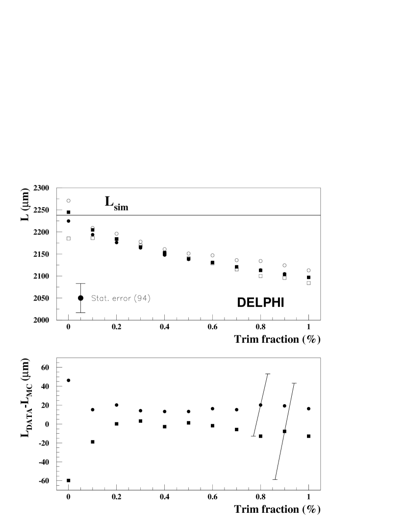
The above mentioned outlier rejection, performed by trimming of the residuals, introduced an additional bias since the asymmetric exponential tail due to the lifetime distribution was preferentially cut. The effect was significant and the induced shift was derived from simulated event studies. A check was made comparing the behaviour of the decay length fitted on the data with the expectation from the simulation. The fitted decay lengths as a function of the trim fraction are displayed in Fig. 3. There was good agreement between data and simulation, providing a lifetime determination that is stable with respect to changes in the trim fraction. A trimming point of 0.4% was chosen as in previous publications, corresponding to a bias of $-43.4\pm 7.9$ $\mu$ m and $-40.3\pm 6.8$ $\mu$ m for 1994 and 1995 respectively. The uncertainty quoted is the one due to simulation statistics. In order to take into account the uncertainty due to the modeling of the trim dependence in the simulation, a further contribution to the systematic uncertainty was added. It was estimated as the maximum difference between the lifetime evaluated at the chosen trim point and all the other evaluations in the interval [0.1;1.0]%. This amounted to 9 $\mu$ m and 10 $\mu$ m for 1994 and 1995 data respectively.

As an additional systematic check, the point at which the line intercepted the $y$ -axis was determined. This was expected to be different from zero, due to the correlation between the energy loss (particularly relevant for electrons) and the shift in the reconstructed impact parameter. This effect was checked using the lepton identification algorithm described in Section 3.1. Combining the 1994 and 1995 samples, the offsets were $23.0\pm 2.7$ $\mu$ m for events containing at least one identified electron and $3.9\pm 1.4$ $\mu$ m for events with no identified electrons. These results agreed well with the expectations from the simulation of $20.6\pm 0.7$ $\mu$ m and $5.4\pm 0.6$ $\mu$ m respectively.

The bias induced by the background was estimated by adding to a simulated sample 50 samples of simulated background events which had passed the selection criteria. The average bias was $-11.4\pm 4.9$ $\mu$ m for 1994 and $-17.5\pm 7.4$ $\mu$ m for 1995, where the systematic uncertainty was the r.m.s. of the biases calculated in each of the 50 samples. Additional systematic uncertainties were due to the uncertainty on the resolution function (3.8 $\mu$ m) and to the vertex detector alignment. The latter was checked by computing the lifetime using a vertex detector geometrical description simulating the alignment uncertainties. Most parameters are well constrained by the alignement procedure and provide negligible variation in the lifetime determination. Only the less constrained deformation, a coherent radial variation of the silicon ladders, provided a visible shift in the reconstructed values, which amounted to 3.1 $\mu$ m, for a radial movement of 20 $\mu$ m. These results are in qualitative agreement with what obtained from a simplified simulation in section 5.3 of [20].

	1994	1995	Correlation
	[fs]	[fs]	coefficient
Fit result	$281.1\pm 4.3$	$279.7\pm 6.7$	0
Syst. sources:
Method bias	$+3.5\pm 0.2$	$+3.5\pm 0.2$	1
Trim	$+5.6\pm 1.0$	$+5.2\pm 0.9$	0
Trim data/MC agreement	$\pm 1.2$	$\pm 1.3$	0
Background	$+1.5\pm 0.6$	$+2.3\pm 1.0$	0.45
Alignment	$\pm 0.4$	$\pm 0.4$	0
Resolution	$\pm 0.5$	$\pm 0.5$	1
Result	$291.7\pm 4.3\pm 1.8$	$290.7\pm 6.7\pm 2.0$	0.02
Average 94+95	$\mathbf{2}91.4\pm 3.6\pm 1.5$

Table 4: Summary of results, correction for biases, systematic uncertainties and combination of the Impact Parameter Difference measurements.

The uncertainty due to the resolution function was considered to be correlated between the two years and a correlation of 0.45 was calculated for the uncertainty due to the background. All the other systematic uncertainties were uncorrelated, as they came from calibrations which were computed with different data sets for the two samples. A summary of all systematic uncertainties is given in Table 4. The lifetimes were measured to be:

$\displaystyle\tau_{\tau}\mbox{(IPD, 94)}$	$\displaystyle=$	$\displaystyle 291.7\pm 4.3_{stat}\pm 1.8_{sys}\mbox{\ fs},$
$\displaystyle\tau_{\tau}\mbox{(IPD, 95)}$	$\displaystyle=$	$\displaystyle 290.7\pm 6.7_{stat}\pm 2.0_{sys}\mbox{\ fs},$
$\displaystyle\tau_{\tau}\mbox{(IPD, 94+95)}$	$\displaystyle=$	$\displaystyle 291.4\pm 3.6_{stat}\pm 1.5_{sys}\mbox{\ fs}.$

3.3 The Miss Distance Method

At LEP, the algebraic sum of the impact parameters, $\delta=d_{+}+d_{-}$ , named the “miss distance”, was strongly correlated to the separation of the two tracks at the production point. The width of the miss distance distribution for one-prong versus one-prong tau decays depends on the value of the lifetime. This was measured by an unbinned maximum likelihood fit to the observed distribution. The probability density function was given by the convolution of a physics function and a resolution function.

The physics function was given by the distribution of miss distances expected from the decay length of $\tau$ ’s. This was built from the convolution of the impact parameter distribution of tracks originating from $\tau^{+}$ decays with that of tracks originating from $\tau^{-}$ decays.

The dependence of the impact parameter distribution upon the track momentum, the decay kinematics and the $\tau$ helicity was also considered. The differences in the distribution for leptons and hadrons depend on the different $\tau$ decay kinematics in one-prong topologies; while leptonic tau decays have three final-state particles, hadronic decays have two or more depending on the number of neutral particles present in the decay. These differences are important for momenta less than 20 GeV/ $c$ .

The shape of the single impact parameter distribution, as a function of decay dynamics and kinematics, was determined on a sample of 185842 simulated events which passed all the selection and quality cuts; it was parameterized as a linear combination of three exponentials.

To obtain the miss distance, the convolution of the two functions describing the single impact parameter distribution, $f_{IP\>+}(d_{+})$ for the $\tau^{+}$ and $f_{IP\>-}(d_{-})$ for the $\tau^{-}$ , was calculated. Since the helicities were not known for a single event, the function was calculated as the sum of the physics function for positive helicity events and the one for negative helicity events, mixed according to the $\tau$ polarisation [21].

To compute the lifetime, the physics function was convoluted with the experimental uncertainties on the reconstruction of the miss distance. As the lifetime information was only in the width of the miss distance distribution, and not in its average value, the increase in width induced by the reconstruction uncertainties had to be evaluated with high precision. In particular it was essential to have a good modeling of the tails due to scattering of the particles through the apparatus.

The resolution was determined for the single impact parameter and then convoluted to provide the miss distance. Hadrons and leptons required different resolution functions, as can be seen in Fig. 4, where the variance of the pull distribution of the reconstructed impact parameter is plotted against $p_{\mbox{\scriptsize norm}}$ , for the simulated tau sample. The pull is defined as the difference between the generated and reconstructed impact parameter divided by the tracking uncertainty given by the reconstruction program. The variable $p_{\mbox{\scriptsize norm}}$ is defined as

p_{\mbox{\scriptsize norm}}=\frac{p}{E_{\mbox{\scriptsize beam}}}\left(2-\frac{p}{E_{\mbox{\scriptsize beam}}}\right),

(15)

where $p$ is the particle momentum. This variable was chosen because its distribution is almost flat for tau decays.

Fig. 4 shows that the average value of the variance of the pull is different from unity. This was due to the presence of tails in the impact parameter distribution. At low momenta all types of particles had similar precision since the dominant effect was multiple Coulomb scattering while at high momenta the different interactions of the particles show up in a difference in resolution. The momentum dependence of the variance of the impact parameter pull for hadrons was much less than that for muons and electrons. This was a consequence of the tuning procedure used to obtain the tracking uncertainties, which was based largely on (both simulated and real data) samples of hadrons in multi-hadronic Z decays.

To have an acceptable description of the resolution function, a three-Gaussian parameterization,

f_{\mbox{\scriptsize res}}(d|p,\theta)=\sum_{i=1}^{3}f_{i}(p,\theta)G\left(d|\sigma_{i}(p,\theta)\right),

(16)

was used. Both the relative fractions $f_{i}$ and widths $\sigma_{i}$ of the Gaussians were dependent on the momentum and polar-angle, as explained below.

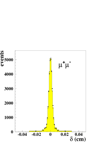
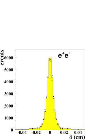
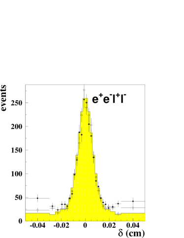
The resolution function was calibrated on the data. This required event samples with a topology similar to that of one-prong tau decays but with no lifetime effect. Applying the same track quality cuts and lepton identification as for the tau pair selection, but appropriately choosing the $P_{\mbox{\scriptsize rad}}$ and $E_{\mbox{\scriptsize rad}}$ cuts, it was possible to select samples with e⁺e^- and $\mu^{+}\mu^{-}$ pairs, produced by e⁺e^- annihilation at high energy, and by $\gamma\gamma$ interactions at low energy. The obtained purities where 98.2% for the high energy e⁺e^- pairs, 99.4% for the high energy $\mu^{+}\mu^{-}$ pairs and 94% for the low energy lepton pairs. The approach chosen was to use the data for the estimation of the resolution at high and low momenta and the simulation to interpolate in the intermediate momentum region. The parameterization used was

\begin{array}[]{lcllcl}f_{1}&=&(1-\alpha)f_{mh}f_{th}+\alpha f_{ml}f_{tl},&\sigma_{1}&=&[(1-\alpha)k_{1h}+\alpha k_{1l}]\sigma_{\mbox{\scriptsize 0}},\\ f_{2}&=&(1-\alpha)(1-f_{mh})f_{th}+\alpha(1-f_{ml})f_{tl},&\sigma_{2}&=&[(1-\alpha)k_{2h}+\alpha k_{2l}]\sigma_{\mbox{\scriptsize 0}},\\ f_{3}&=&(1-\alpha)(1-f_{th})+\alpha(1-f_{tl}),&\sigma_{3}&=&[(1-\beta)k_{3h}+\beta k_{3l}]\sigma_{\mbox{\scriptsize 0}},\\ \end{array}

(17)

where

\alpha=\left[1-\frac{p\sin^{3/2}\theta}{E_{\mbox{\scriptsize beam}}}\left(2-\frac{p\sin^{3/2}\theta}{E_{\mbox{\scriptsize beam}}}\right)\right]^{a},

(18)

\beta=\left[1-\frac{p\sin^{3/2}\theta}{E_{\mbox{\scriptsize beam}}}\left(2-\frac{p\sin^{3/2}\theta}{E_{\mbox{\scriptsize beam}}}\right)\right]^{b}.

(19)

and $\sigma_{\mbox{\scriptsize 0}}$ is the uncertainty estimation from the b-tagging package [16]. The parameters $f_{mh}$ , $f_{th}$ , $k_{1h}$ , $k_{2h}$ , $k_{3h}$ and $f_{ml}$ , $f_{tl}$ , $k_{1l}$ , $k_{2l}$ , $k_{3l}$ were determined from the miss distance distribution at high and low momentum respectively. As an example the fitted distributions for the 1994 data sample are shown in Figure 5. The parameters $\alpha$ and $\beta$ range from 1 at low momentum to 0 at high momentum. The steepness of the change was controlled by the parameters $a$ and $b$ , derived from the simulation. For hadrons an exponential contribution was added in order to take into account the effect of elastic hadronic interactions.

The lifetime was determined by an unbinned maximum likelihood fit to the observed distribution, where the probability density function was given by the convolution of the physics function and the resolution function described above. The entire procedure was tested on simulated samples from which a bias of $-0.2~{}\pm~{}0.9$ fs was measured.

Fig. 6 shows the joint distribution of the miss distance for 1994 and 1995 data, with the best fit superimposed. The measured lifetimes, including all the corrections, are

	$\displaystyle\tau_{\tau}\mbox{(MD, 94)}$	$\displaystyle=$	$\displaystyle 292.5\pm 2.8_{stat}\pm 2.3_{sys}\mbox{\ fs},$
	$\displaystyle\tau_{\tau}\mbox{(MD, 95)}$	$\displaystyle=$	$\displaystyle 291.0\pm 4.0_{stat}\pm 2.3_{sys}\mbox{\ fs}.$

The sources of systematic uncertainties are listed in Table 5. The event selection criteria were varied inducing a lifetime change of 1.1 fs in 1994 and 1.0 fs in 1995. The influence of the physics function and resolution function was checked by varying by $\pm 1\sigma$ the parameters of the functions parameterization, taking into account correlations. A further contribution to the resolution function, due to hadronic scattering, was evaluated comparing the data and simulation for hadronic events. The residual lepton misidentification, after applying the procedure in section 3.1 resulted in a systematic uncertainty of $\pm 0.2$ fs. The effect of background from e⁺e^-, $\mu^{+}\mu^{-}$ and $\gamma\gamma$ events was evaluated using simulated samples that passed all the selection cuts, resulting in estimated biases of $-0.6\pm 0.4$ fs in 1994 and $-0.8\pm 0.4$ fs in 1995. The contribution to the systematic uncertainty due to the alignment of the Microvertex Detector, estimated using the same procedure as in section 3.2, was 0.5 fs. The dependence on the tau polarization $P_{\tau}$ was checked by varying it in the range $[-0.11;-0.17]$ resulting in a $\pm 0.1$ fs variation on the lifetime, while the effect of the transverse polarisation correlation was evaluated as $\pm 0.4$ fs [2]. The fit was performed over the range $|\delta|<1.5$ mm. This range was varied between $|\delta|<1$ mm and $|\delta|<2$ mm to study the systematic effect. The maximum difference observed was taken as a systematic uncertainty.

	1994	1995	Correlation
	[fs]	[fs]	coefficient
Fit result	$291.7\pm 2.8$	$290.0\pm 4.0$	0.0
Syst. Sources:
Method bias	$+0.2\pm 0.9$	$+0.2\pm 0.9$	1.0
Event Selection	$\pm 1.1$	$\pm 1.0$	0.0
Physics Function	$\pm 0.8$	$\pm 0.8$	1.0
Resolution Function	$\pm 1.3$	$\pm 1.5$	0.9
Particle Misidentification	$\pm 0.2$	$\pm 0.2$	1.0
Background	$+0.6\pm 0.4$	$+0.8\pm 0.4$	0.7
Alignment	$\pm 0.5$	$\pm 0.5$	0.0
Polarisation	$\pm 0.4$	$\pm 0.4$	1.0
Fit Range	$\pm 0.7$	$\pm 0.2$	0.0
Result	$292.5\pm 2.8\pm 2.3$	$291.0\pm 4.0\pm 2.3$	0.17
Average 94+95	$\mathbf{2}92.0\pm 2.3\pm 2.1$

Table 5: Summary of results, correction for biases, systematic uncertainties and combination of the Miss Distance measurements.

The measurements for the two years were combined, accounting for the correlations in the systematic uncertainties shown in Table 5, to give the result

\tau\mbox{(MD, 94-95)}=292.0\pm 2.3_{stat}\pm 2.1_{sys}\mbox{\ fs.}

4 Combination of Measurements

The lifetime of the tau has been measured with three methods. The two one-prong measurements were performed on the same data sample and were combined taking into account correlated statistical and systematic uncertainties. The statistical correlation was obtained by subdividing the simulated data into 89 samples of 5000 events, applying the two analysis methods on each sample and computing the correlation coefficient as:

\rho=\frac{\sum_{i}(\tau_{{\mbox{\scriptsize IPD}},i}-\tau_{\tau})(\tau_{{\mbox{\scriptsize MD}},i}-\tau_{\tau})}{\sqrt{\sum_{i}(\tau_{{\mbox{\scriptsize IPD}},i}-\tau_{\tau})^{2}\sum_{i}(\tau_{{\mbox{\scriptsize MD}},i}-\tau_{\tau})^{2}}},

(20)

where $\tau_{{\mbox{\scriptsize IPD}},i}$ and $\tau_{{\mbox{\scriptsize MD}},i}$ are the determined lifetimes for each sample respectively with the impact parameter difference and the miss distance methods, and $\tau_{\tau}$ is the simulated lifetime. The resulting statistical correlation was 36%. Among the systematic uncertainties only the background estimation and alignment contribution were correlated. This provides a combined result of

\tau_{\tau}\mbox{(1-prong, 94+95)}=291.8\pm 2.3_{stat}\pm 1.5_{sys}\mbox{\ fs.}

This measurement was averaged with previously published DELPHI results [2, 4]:

	$\displaystyle\tau_{\tau}\mbox{(1-prong, 91)}$	$\displaystyle=$	$\displaystyle 298\pm 7_{stat}\pm 4_{sys}\mbox{\ fs},$
	$\displaystyle\tau_{\tau}\mbox{(1-prong, 92--93)}$	$\displaystyle=$	$\displaystyle 291.8\pm 3.3_{stat}\pm 2.1_{sys}\mbox{\ fs},$

to provide the result for all LEP-1 DELPHI data for the one-prong methods:

\tau_{\tau}\mbox{(1-prong, 91-95)}=292.3\pm 1.8_{stat}\pm 1.2_{sys}\mbox{\ fs}.

The final one-prong estimation was combined with the three-prong measurement to give the best estimation of the tau lifetime from the DELPHI data. Only the systematic uncertainty attributed to the alignment of the vertex detector is common between the one-prong and three-prong measurements, resulting in a 5% correlation between the two results. By combining the two results and taking into account this correlation, a tau lifetime of

\tau_{\tau}=290.9\pm 1.4_{stat}\pm 1.0_{sys}\mbox{\ fs}

was obtained.

5 Summary and Conclusions

The tau lifetime has been measured using the DELPHI LEP-1 data sample. The result

\tau_{\tau}=290.9\pm 1.4_{stat}\pm 1.0_{sys}\mbox{\ fs}

was obtained. This result supersedes all previous DELPHI measurements of the tau lifetime. The measurement is compatible with the values published by other experiments [22] and has a slightly better precision.

Tests of $\tau-\mu$ and $\tau-{\rm{e}}$ universality can be performed using this result in conjunction with the published DELPHI values for the $\tau$ leptonic branching fractions [23]:

B(\tau^{-}\rightarrow\rm e^{-}\bar{\nu_{\rm e}}\nu_{\tau})=(17.877\pm 0.109_{stat}\pm 0.110_{sys})\%,

B(\tau^{-}\rightarrow\mu^{-}\bar{\nu_{\mu}}\nu_{\tau})=(17.325\pm 0.095_{stat}\pm 0.077_{sys})\%,

together with the world average values of the lepton masses and the muon lifetime [5]. Using equations (1) and (2), and accounting for small radiative corrections (see [23] for a discussion), yielded

\frac{g_{\tau}}{g_{\mu}}=1.0015\pm 0.0053,

\frac{g_{\tau}}{g_{e}}=0.9997\pm 0.0046.

The branching fraction measurements contributed to the uncertainty in these estimates with $\pm 0.0043$ and $\pm 0.0035$ respectively.

Under the assumption of e- $\mu$ universality, $g_{\mu}=g_{e}\equiv g_{{\rm e},\mu}$ , it was possible to give a more stringent test of universality of the coupling of the $\tau$ and that of the two lighter leptons. The two measurements were combined into one leptonic branching fraction, $B_{e,\mu}$ , correcting for the phase space suppression of $B(\tau^{-}\rightarrow\mu^{-}\bar{\nu_{\mu}}\nu_{\tau})$ :

B_{e,\mu}=(17.838\pm 0.066_{stat}\pm 0.068_{sys})\%,

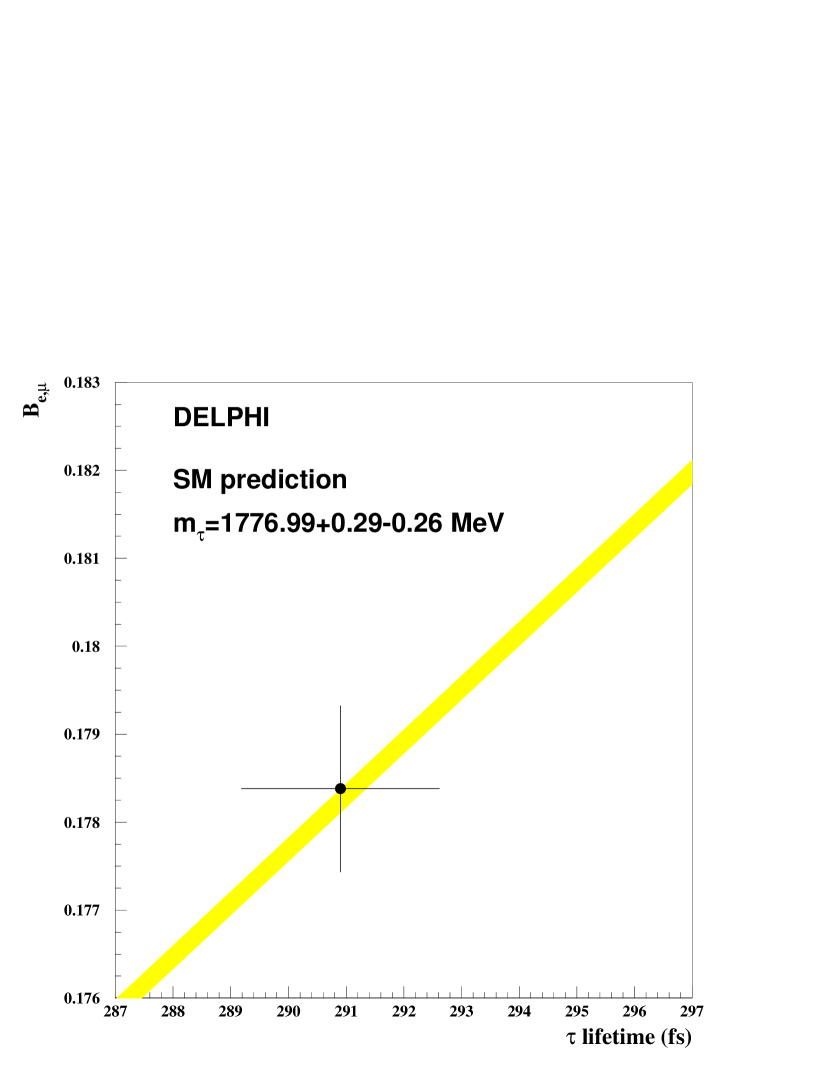
to compare the tau charged current coupling to that of the two lighter leptons. The result

\frac{g_{\tau}}{g_{{\rm e},\mu}}=1.0004\pm 0.0041

was obtained, in excellent agreement with $\tau$ - $(e,\mu)$ universality. The relation between the leptonic branching ratio and the $\tau$ lifetime is shown in Fig. 7, under the assumption of $e$ - $\mu$ universality. The band reflects the uncertainty on the tau mass [5].

Acknowledgements

We are greatly indebted to our technical collaborators, to the members of the CERN-SL Division for the excellent performance of the LEP collider, and to the funding agencies for their support in building and operating the DELPHI detector.
We acknowledge in particular the support of
Austrian Federal Ministry of Education, Science and Culture, GZ 616.364/2-III/2a/98,
FNRS–FWO, Flanders Institute to encourage scientific and technological research in the industry (IWT), Belgium,
FINEP, CNPq, CAPES, FUJB and FAPERJ, Brazil,
Czech Ministry of Industry and Trade, GA CR 202/99/1362,
Commission of the European Communities (DG XII),
Direction des Sciences de la Mati $\grave{\mbox{\rm e}}$ re, CEA, France,
Bundesministerium f $\ddot{\mbox{\rm u}}$ r Bildung, Wissenschaft, Forschung und Technologie, Germany,
General Secretariat for Research and Technology, Greece,
National Science Foundation (NWO) and Foundation for Research on Matter (FOM), The Netherlands,
Norwegian Research Council,
State Committee for Scientific Research, Poland, SPUB-M/CERN/PO3/DZ296/2000, SPUB-M/CERN/PO3/DZ297/2000, 2P03B 104 19 and 2P03B 69 23(2002-2004)
FCT - Fundação para a Ciência e Tecnologia, Portugal,
Vedecka grantova agentura MS SR, Slovakia, Nr. 95/5195/134,
Ministry of Science and Technology of the Republic of Slovenia,
CICYT, Spain, AEN99-0950 and AEN99-0761,
The Swedish Natural Science Research Council,
Particle Physics and Astronomy Research Council, UK,
Department of Energy, USA, DE-FG02-01ER41155.
EEC RTN contract HPRN-CT-00292-2002.

References

[1] Y.S. Tsai, Phys. Rev. D4 (1971) 2821.
H.B. Thacker and J.J. Sakurai, Phys. Lett. B36 (1971) 103.
[2] P. Abreu et al., DELPHI Collaboration, Phys. Lett. B365 (1996) 448.
[3] N. Bingefors et al., Nucl. Instr. and Meth. A328 (1993) 447;
V. Chabaud et al., Nucl. Instr. and Meth. A368 (1996) 314.
[4] P. Abreu et al., DELPHI Collaboration, Phys. Lett. B302 (1993) 356.
[5] K. Hagiwara et al, Phys. Rev. D66 (2002) 010001.
[6] S. Jadach, B. F. L. Ward and Z. Was, Comp. Phys. Comm. 79 (1994) 503.
[7] S. Jadach et al., Comp. Phys. Comm. 76 (1993) 361.
[8] J. E. Campagne and R. Zitoun, Zeit. Phys. C43 (1989) 469.
[9] F. A. Berends, R. Kleiss and W. Hollik, Nucl. Phys. B304 (1988) 712.
[10] S. Jadach, W. Placzek and B. F. L. Ward, Phys. Lett. B390 (1997) 298.
[11] P. Abreu et al., DELPHI Collaboration, Zeit. Phys. C73 (1996) 11.
[12] F. A. Berends, P. H. Daverveldt and R. Kleiss, Phys. Lett. B148 (1984) 489;
F. A. Berends, P. H. Daverveldt and R. Kleiss, Comp. Phys. Comm. 40 (1986) 271.
[13] T. Alderweireld et al., CERN Report CERN-2000-009 (2000) 219.
[14] P. Abreu et al., DELPHI Collaboration, Nucl. Instr. and Meth. A378 (1996) 57.
[15] P. Aarnio et al., DELPHI Collaboration, Nucl. Instr. and Meth. A303 (1991) 233.
[16] P. Abreu et al., DELPHI Collaboration, Eur. Phys. J. C10 (1999) 415.
[17] P. Abreu et al., DELPHI Collaboration, Zeit. Phys. C67 (1995) 183.
[18] P. Abreu et al., DELPHI Collaboration, Phys. Lett. B357 (1995) 715.
[19] D. Decamp et al., ALEPH Collaboration, Phys. Lett. B279 (1992) 411.
[20] S. Wasserbaech, Nucl. Phys. B (Proc. Suppl.) 76 (1999) 107.
[21] P. Abreu et al., DELPHI Collaboration, Eur. Phys. J. C14 (2000) 585.
[22] G. Alexander et al., OPAL Collaboration, Phys.Lett. B374 (1996) 341;
R. Balest et al., CLEO Collaboration, Phys.Lett. B388 (1996) 402;
M. Acciarri et al., L3 Collaboration, Phys.Lett. B479 (2000) 67;
R. Barate et al., ALEPH Collaboration, Phys.Lett. B414 (1997) 362.
[23] P. Abreu et al., DELPHI Collaboration, Eur. Phys. J. C10 (1999) 201.

Refer to caption — Figure 1: Decay length distribution for three-prong tau decays. The points are 1991-1995 data sample and the histogram is the result of the fit.