The BABAR Collaboration

We present a preliminary measurement of $R_{1}$, $R_{2}$, and $\rho^{2}$, which are the three parameters used to characterize the $B\mbox{$\rightarrow$}D^{*}\ell\bar{\nu}_{e}$ form factors ($A_{1}$, $V$, and $A_{2}$). We use $85\times 10^{6}$ $B\bar{B}$-pairs accumulated on the $\mathchar 28935\relax(4{\rm S})$ resonance at PEP-II. In this analysis we use the decay mode $\bar{B}^{0}\mbox{$\rightarrow$}D^{+*}e^{-}\bar{\nu}$ and its charge conjugate. The $D^{*+}$ is reconstructed in the channel $D^{*+}\rightarrow D^{0}\pi^{+}$ and the $D^{0}$ in the channel $D^{0}\rightarrow K^{-}\pi^{+}$. We parameterize the form factors in terms of their ratios (determined by the parameters $R_{1}$ and $R_{2}$) and the common slope $\rho^{2}$ in the variable $w$ (a quantity related to the momentum transfer in the decay process). These parameters are determined via an unbinned maximum likelihood fit to the distributions in four kinematic variables (three decay angles and $w$). The results are $R_{1}=1.328\pm 0.055\pm 0.025\pm 0.025$ and $R_{2}=0.920\pm 0.044\pm 0.020\pm 0.013$ for the ratios and $\rho^{2}=0.769\pm 0.039\pm 0.019\pm 0.032$ for the slope. The stated errors are the statistical uncertainty from the data, statistical uncertainty from the size of the Monte Carlo sample and the systematic uncertainty, respectively.

1 Introduction

The decay $B\mbox{$\rightarrow$}D^{*}\ell\nu$ can be described by three form factors: two axial form factors, $A_{1}$ and $A_{2}$, and one vector form factor, $V$. They are functions of the momentum transfer $q^{2}$ (or equivalently, $w$, defined below). Measurements of these form factors provide us with a “laboratory” for testing the predictions of heavy quark effective theory (HQET) [1]. These form factors are related to each other by heavy quark symmetry (HQS) through the formalism of heavy quark effective theory. Deviations from the HQET relationships can be computed as corrections to the theory. They can also in principle be measured; the parameters we adopt for this analysis are inspired by HQET, but allow for such deviations.

We introduce here a novel method of extracting these parameters from the data. We use an unbinned-maximum-likelihood method, but introduce approximations that allow us to correct efficiency and resolution with the limited Monte Carlo (MC) data sample available. In Sec. 6 we sketch out how these approximations work and how we evaluate their impact on the errors.

Improved measurements of the form factor parameters $R_{1}$, $R_{2}$ and $\rho^{2}$ yield a significant reduction in the systematic error obtainable on the Cabibbo-Kobayashi-Maskawa (CKM) matrix element $V_{cb}$. In this analysis, though we restrict ourselves to the cleanest available decay channel, we still obtain nearly 17 times as many reconstructed $B\mbox{$\rightarrow$}D^{*}\ell\nu$ decay candidates as the pioneering CLEO analysis [2]. This already produces a substantial improvement in the error achieved on the parameters $R_{1}$ and $R_{2}$ needed for extracting $V_{cb}$. Further, a better understanding of this channel, which is the dominant background to $B\rightarrow X_{u}\ell\nu$, is also of great importance to the study of inclusive and exclusive $B\rightarrow X_{u}\ell\nu$ decays and the determination of $V_{ub}$.

With the addition of more data and the use of the other available decay modes we will be able to further probe the consistency of HQET predictions in the near future.

2 Formalism

The Feynman diagram for the decay ${\bar{B}}^{0}\rightarrow D^{*+}\ell^{-}\overline{\nu}$ is shown in Fig. 1.

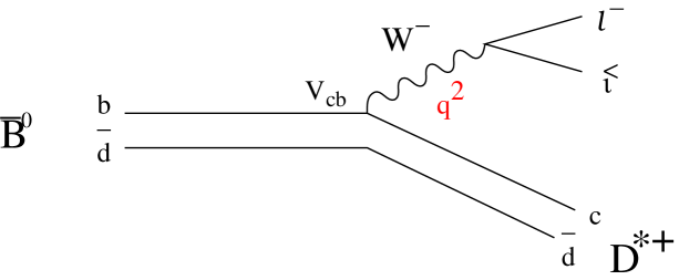
Figure 1: Quark level diagram that leads to the decay ${\bar{B}^{0}\rightarrow D^{*}\ell\nu}$ .

The square of momentum transfer from the $B$ to the $D^{*}$, $q^{2}$, is linearly related to another Lorentz invariant ($w$) by

$$\mbox{${w}$}\equiv{M_{B}^{2}+M_{D^{*}}^{2}-q^{2}\over 2M_{B}M_{D^{*}}}=v_{B}\cdot v_{D^{*}}={p_{B}\cdot p_{D^{*}}\over M_{B}M_{D^{*}}}$$ (1)

where $M_{B}$ and $M_{D^{*}}$ are the masses of the $B$ and the $D^{*}$ mesons, $p_{B}$ and $p_{D^{*}}$ are their four momenta, and $v_{B}$ and $v_{D^{*}}$ are their four-velocities. In the $B$ rest frame $w$ reduces to the Lorentz boost factor $\gamma_{D^{*}}=(E_{D^{*}}/M_{D^{*}})$.

The range of $w$ and $q^{2}$ are restricted by the kinematics of the decay with $q^{2}=0$ corresponding to

$$w_{max}=\frac{M_{B}^{2}+M_{D^{*}}^{2}}{2M_{B}M_{D^{*}}}\approx 1.504$$ (2)

and $w_{min}=1$ corresponding to

$$q_{max}^{2}=(M_{B}-M_{D^{*}})^{2}\approx 10.69({\mathrm{\,Ge\kern-1.00006ptV\!/}c^{2}})^{2}.$$ (3)

2.1 Kinematic Variables

We choose to reconstruct the mode where the $D^{*}$ decays to $D\pi$, and the $D$ to a $K\pi$ . The outgoing particles are shown in Fig. 2. The pion from the $D^{*}$ decay and the electron are directly detected, and the $D$ is reconstructed from its daughters, the $K$ and $\pi$.

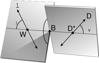
Figure 2: Kinematics of $B\mbox{$\rightarrow$}D^{*}\ell\nu$  decays.

In Fig. 2 we define three angles, which, along with ${w}$, constitute the four independent kinematic variables we use to characterize this decay:

• ${\cos\theta_{\ell}}$, the cosine of the angle between the direction of the lepton in the virtual $W$ rest frame, and the direction of the virtual $W$ in the $B$ rest frame

• ${\cos\theta_{V}}$, the cosine of the angle between the direction of the $D$ in the $D^{*}$ rest frame, and the direction of the $D^{*}$ in the B rest frame

• ${\chi}$, the azimuthal angle between the plane formed by the $\mbox{$D^{*}$}-D$ system and the plane formed by the $W-\ell$ system.

A $D^{*}\ell\nu$ decay is completely characterized by the four kinematic variables $w$, ${\cos\theta_{\ell}}$, ${\cos\theta_{V}}$ and $\chi$. Since the $B$ meson is spinless, the direction of the $D^{*}-W$ axis relative to the $B$ direction is irrelevant to the dynamics.

2.2 Four Dimensional Decay Distribution

2.2.1 Helicity amplitudes

The Lorentz structure of the $B\mbox{$\rightarrow$}D^{*}\l\nu$ decay amplitude can be expressed in terms of three amplitudes ($\mbox{$H$}_{+}$, $\mbox{$H$}_{-}$, and $\mbox{$H$}_{0}$), which correspond to the three allowed polarization states of the $D^{*}$ (two transverse and one longitudinal). These amplitudes can be completely specified in terms of the axial and vector form factors as follows[1]:

$$\mbox{$H$}_{+}(w)\equiv-(M_{B}+M_{D^{*}}){A_{1}(w)}+2{\wp_{D^{*}}M_{B}\over M_{B}+M_{D^{*}}}{V(w)},$$ (4)

$$\mbox{$H$}_{-}(w)\equiv-(M_{B}+M_{D^{*}}){A_{1}(w)}-2{\wp_{D^{*}}M_{B}\over M_{B}+M_{D^{*}}}{V(w)},$$ (5)

$$\mbox{$H$}_{0}(w)\equiv-{1\over 2M_{D^{*}}\sqrt{q^{2}}}\left[{A_{1}(w)}(M_{B}+M_{D^{*}})(M_{B}^{2}-M_{D^{*}}^{2}-q^{2})-\right.$$ (6)

$$\left.4{M_{B}^{2}\wp_{D^{*}}^{2}\over M_{B}+M_{D^{*}}}{A_{2}(w)})\right],$$

where $\wp_{D}^{*}=M_{D^{*}}\sqrt{w^{2}-1}$ is the magnitude of the momentum of the $D^{*}$ in the $B$ rest frame.

By contracting the relevant lepton and hadron tensors, neglecting small terms of order $m^{2}_{\ell}/q^{2}$, and doing the phase space integrations, the full differential decay rate

$${d\Gamma(B\mbox{$\rightarrow$}\mbox{$D^{*}\ell\nu$})\over dw\;d\mbox{${\cos\theta_{\ell}}$}\;d\mbox{${\cos\theta_{V}}$}\;d\chi} = {6G^{2}_{F}|V_{cb}|^{2}M_{B}M_{D^{*}}^{2}r\sqrt{(w^{2}-1)}(1-2wr+r^{2})\over 8(4\pi)^{4}}\times$$

$$\left[{H_{+}}^{2}(1-\mbox{${\cos\theta_{\ell}}$})^{2}\sin^{2}\theta_{V}+{H_{-}}^{2}(1+\mbox{${\cos\theta_{\ell}}$})^{2}\sin^{2}\theta_{V}\right.$$

$$+4{H_{0}}^{2}\sin^{2}\theta_{\ell}\cos^{2}\theta_{V}-2{H_{+}H_{-}}\sin^{2}\theta_{\ell}\sin^{2}\theta_{V}\cos(2\chi)$$

$$-4{H_{+}H_{0}}\mbox{${\sin\theta_{l}}$}(1-\mbox{${\cos\theta_{\ell}}$})\mbox{${\sin\theta_{V}}$}\mbox{${\cos\theta_{V}}$}\cos\chi$$

$$\left.+4{H_{-}H_{0}}\mbox{${\sin\theta_{l}}$}(1+\mbox{${\cos\theta_{\ell}}$})\mbox{${\sin\theta_{V}}$}\mbox{${\cos\theta_{V}}$}\cos\chi\right]$$

can be obtained in terms of the helicity amplitudes. Here $r\equiv{\left(M_{D^{*}}\over M_{B}\right)}$ is the ratio of the $D^{*}$ to the $B$ mass. Details of the derivation can be found in Neubert[1]. The four-dimensional distribution of $w$, ${\cos\theta_{\ell}}$ ${\cos\theta_{V}}$ and $\chi$ that is described by Eq.(2.2.1) is the physical observable from which we can extract the form factors.

2.2.2 Heavy Quark Symmetry Relationships

HQS relates the three form factors to each other, as follows:

$$A_{2}(w)=\frac{R_{2}(w)}{R^{*2}}\frac{2}{w+1}A_{1}(w),$$ (8)

$$V(w)=\frac{R_{1}(w)}{R^{*2}}\frac{2}{w+1}A_{1}(w),$$ (9)

where we have defined the constant

$$R^{*}\equiv{{2\sqrt{M_{B}M_{D^{*}}}}\over{(M_{B}+M_{D^{*}})}}.$$ (10)

$R_{1}(w)=R_{2}(w)=1.0$, i.e., perfect HQS, implies that the form factors, $A_{2}$ and $V$ are identical for all values of $w$. Since HQS is not exact, $R_{1}$ and $R_{2}$ can differ from $1.0$ and exhibit some $w$-dependence.

$A_{1}$ can be related to the Isgur-Wise function by

$$A_{1}(w)=R^{*}\frac{w+1}{2}h_{A_{1}}(w),$$ (11)

where in the HQET limit $h_{A_{1}}$ is the Isgur-Wise function $\xi(w)$ [3]. HQET predicts $h_{A_{1}}(1)=\xi(1)=1.0$.

It is convenient to re-express the helicity amplitudes $H_{i}$ ($i=\pm,0$) in terms of the functions $R_{1}(w)$ and $R_{2}(w)$ as follows

$$\mathit{\tilde{\mbox{$H$}}_{+}} =\left[{\displaystyle\frac{\sqrt{(1-2\,\mbox{${w}$}\,r+r^{2})}\,\left(1-\sqrt{{\displaystyle\frac{\mbox{${w}$}-1}{\mbox{${w}$}+1}}}\,\mathit{{\mbox{$R_{1}$}}(w)}\right)}{(1-r)}}\right],$$

$$\mathit{\tilde{\mbox{$H$}}_{0}} =\left[1+{\displaystyle\frac{(\mbox{${w}$}-1)\,(1-\mathit{{\mbox{$R_{2}$}}(w)})}{1-r}}\right],$$ (12)

$$\vspace{.5cm}\mathit{\tilde{\mbox{$H$}}_{-}} =\left[{\displaystyle\frac{\sqrt{(1-2\,\mbox{${w}$}\,r+r^{2})}\,\left(1+\sqrt{{\displaystyle\frac{\mbox{${w}$}-1}{\mbox{${w}$}+1}}}\,\mathit{{\mbox{$R_{1}$}}(w)}\right)}{(1-r)}}\right],$$

where the helicity amplitudes that appear in Eqs.(4-6) differ from these only by a common kinematic factor times $h_{A_{1}}$:

$${\mbox{$H$}}_{i}=-M_{B}\frac{R^{*}(1-r^{2})(w+1)}{2\sqrt{1-2wr+r^{2}}}h_{\mbox{$A$}_{1}}(w)\tilde{H}_{i}$$ (13)

.

The function $h_{A_{1}}(w)$ can be conveniently parameterized by exploiting the fact that $w-1$ is a small parameter (${~{}\raise 1.49994pt\hbox{$<$}\kern-8.50006pt\lower 3.50006pt\hbox{$\sim$}~{}}0.5$) to express it as a power series expansion

$$h_{A_{1}}(w)=h_{A_{1}}(1)\left(1-\rho^{2}(w-1)+c(w-1)^{2}+...\right)$$ (14)

where $\rho^{2}$ is called the slope and $c$ is called the curvature (note that in the literature $\rho^{2}$ is often referred to as $\rho^{2}_{A_{1}}$). Corrections to HQET modify $h_{A_{1}}(1)$ and thus lead to deviations from the HQET limit of $h_{A_{1}}=1.0$. However, in this analysis we only deal with the shape and relative normalization of the form factors, and consequently the overall normalization is irrelevant.

For this preliminary analysis we only use the expansion to first order in $(w-1)$, so we set $c=0$. In our baseline analysis we treat $R_{1}$ and $R_{2}$ as constant. However, we also show results in which we extend the analysis to explore the impact of $w$-dependence.

2.3 Form Factor Predictions

As discussed in Sec. 2.2.2, for infinitely massive $b$ and $c$ quarks, we expect ${\mbox{$R_{1}$}}={\mbox{$R_{2}$}}=1.0$, but for finite masses they are modified by both perturbative $\alpha_{s}\$ and non-perturbative ${\left({\mathchar 28931\relax_{\rm QCD}\over m_{x}}\right)}$ corrections.

Calculating higher-order loop corrections to the form factors yields expansions of the form:

$${{\mbox{$R_{1}$}}}(w) = 1+\left[\mbox{$\alpha_{s}\ $}(...)+\mbox{$\alpha_{s}^{2}\ $}(...)\right]+{\left({\mathchar 28931\relax_{\rm QCD}\over m_{x}}\right)}(...),$$ (15)

$${{\mbox{$R_{2}$}}}(w) = 1+\left[\mbox{$\alpha_{s}\ $}(...)+\mbox{$\alpha_{s}^{2}\ $}(...)\right]+{\left({\mathchar 28931\relax_{\rm QCD}\over m_{x}}\right)}(...).$$ (16)

The coefficients of the $\alpha_{s}\$ terms (shown as ellipses) have been calculated perturbatively up to second order, which gives confidence that they are accurate to about one percent (see [5]). The coefficients of the ${\left({\mathchar 28931\relax_{\rm QCD}\over m_{x}}\right)}$ terms are combinations of quantities called “subleading Isgur-Wise functions.”

Different models in the HQET framework evaluate the subleading Isgur-Wise function correction terms differently, resulting in a variety of predictions for ${\mbox{$R_{1}$}}(w)$ and ${\mbox{$R_{2}$}}(w)$. Neubert [1], based on work with collaborators, in the early 90’s predicted

$${\mbox{$R_{1}$}}(\mbox{${w}$}) = 1.35-0.22(w-1)+0.09(w-1)^{2},$$ (17)

$${\mbox{$R_{2}$}}(\mbox{${w}$}) = 0.79+0.15(w-1)-0.04(w-1)^{2}.$$ (18)

More recently, Caprini et.al. [4] using spectral functions, dispersion relations, and heavy quark symmetry to evaluate the non-perturbative terms predict

$${{\mbox{$R_{1}$}}}(w) = 1.27-0.12(w-1)+0.05(w-1)^{2},$$ (19)

$${{\mbox{$R_{2}$}}}(w) = 0.80+0.11(w-1)-0.06(w-1)^{2}.$$ (20)

Ligeti and Grinstein [5] using similar HQET machinery find

$${{\mbox{$R_{1}$}}}(w) = 1.25-0.10(w-1),$$ (21)

$${{\mbox{$R_{2}$}}}(w) = 0.81+0.09(w-1).$$ (22)

Whereas all the above HQET-based predictions predict form factor values within a fairly narrow range, older predictions relying on ad-hoc potential models vary widely, e.g., Close & Wambach using a simple quark model predict [6]

$${{\mbox{$R_{1}$}}}(w) = 1.15-0.07(w-1),$$ (23)

$${{\mbox{$R_{2}$}}}(w) = 0.91+0.04(w-1).$$ (24)

It can be seen that in all the above predictions the coefficients of the $(w-1)$ and $(w-1)^{2}$ terms are quite small because $R_{1}$ and $R_{2}$ are by construction as ratios expected to vary only slightly with $w$, where $h_{A_{1}}$ has no such restriction.

3 The BABAR Detector and Dataset

The data set used in this analysis was collected with the BABAR detector at the PEP-II storage ring during the period between 2000 and 2002. It corresponds to $84\mbox{ $\rm fb^{-1}$}$ collected on the $\mathchar 28935\relax(4{\rm S})$ resonance, which yields approximately $85\times 10^{6}$ $B\bar{B}$-pairs. There are $\approx 8.5\times 10^{6}$ ${B^{0}\rightarrow D^{*}\ell\nu}$ decays in this sample of which we have reconstructed 16,386 $\bar{B}^{0}\mbox{$\rightarrow$}D^{*+}e^{-}\bar{\nu}_{e}$ (or charge conjugate) candidates using only the $D^{0}\pi^{+}$ decay of the $D^{*}$ and the $K^{-}\pi^{+}$ decay mode of the $D^{0}$.

The BABAR detector is described elsewhere in detail [7]. This analysis uses four of the five subdetectors of BABAR: the silicon vertex tracker, the drift chamber, a Cerenkov-light-based particle identification detector, and the electromagnetic calorimeter. This analysis depends critically on the silicon vertex tracker to reconstruct the low momentum pions produced by the decay $D^{*+}\rightarrow D^{0}\pi^{+}$, about two-thirds of which do not traverse more than about a fourth of the drift chamber.

4 Reconstruction and Event Selection

We reconstruct the lepton, and the $D^{*}$ through its decay products. After reconstruction of all tracks, we choose cuts that select $B\mbox{$\rightarrow$}D^{*}\ell\nu$ decays and determine the kinematic variables $w$, ${\cos\theta_{\ell}}$, ${\cos\theta_{V}}$ and $\chi$.

4.1 Event selection

In this analysis we only consider the decay channel $D^{*+}e^{-}\bar{\nu}_{e}$ with the $D^{*+}$ decaying to $D^{0}\pi^{+}$ and the $D^{0}$ decaying in the $K^{-}\pi^{+}$ mode. In case of multiple $D^{*}e\nu$ candidates in a given event we choose the candidate with $K\pi$ mass ($m_{K\pi}$) closest to the $D^{0}$ mass.

For event selection we use the procedure developed for our $V_{cb}$ analysis [8], and we also apply the same selection criteria. We summarize the most salient of these cuts here:

• The momentum of the lepton in the center-of-mass (C.M.) frame $p^{*}_{\ell}$ is required to be larger than $1.2{\mathrm{\,Ge\kern-1.00006ptV\!/}c}$. This criterion selects $B$ semi-leptonic decays and suppresses continuum ($c\bar{c}$) and cascade ($b\mbox{$\rightarrow$}c\mbox{$\rightarrow$}\ell$) backgrounds.

• The momentum of the $D^{*}$ in the C.M. frame must be between $0.5$ and $2.5{\mathrm{\,Ge\kern-1.00006ptV\!/}c}$.

• The soft pion from the $D^{*}$ decay must have a transverse momentum greater than $50{\mathrm{\,Me\kern-1.00006ptV\!/}c}$.

• The $\chi^{2}$ probability of the fit of the $D^{*}\ell$ vertex to the beamspot constraint must be greater than $1\%$.

• To further suppress continuum background, we select only candidates with $|\cos\theta_{\rm thrust}|<0.85$, where $\theta_{\rm thrust}$ is the angle between the thrust axis of the $D^{*}\ell\nu$ candidate and the thrust axis of the rest of the event.

The cosine of angle $\theta_{BY}$ between the direction of the $B$ and the direction of the $D^{*}-\ell$ system can be computed from the kinematics of the decay (see next Section). Candidates with $\cos\theta_{BY}$ between $-10$ and $+6$ have been used to estimate background. We include only events that have $|\mbox{$\cos\theta_{BY}$}|\leq 1.2$ in the final sample.

The final selection is based on $\mbox{$\delta m$}=m_{K\pi\pi_{s}}-m_{K\pi}$. For candidates in which the $\pi_{s}$ track is reconstructed with twelve or more drift chamber hits we cut on the mass difference $0.144<\mbox{$\delta m$}<0.147$ ${\mathrm{\,Ge\kern-1.00006ptV\!/}c}$. For the less well-measured case with fewer than twelve drift chamber hits we loosen the cut to $0.143<\mbox{$\delta m$}<0.148$ ${\mathrm{\,Ge\kern-1.00006ptV\!/}c}$. About three-quarters of the candidates are in the latter category.

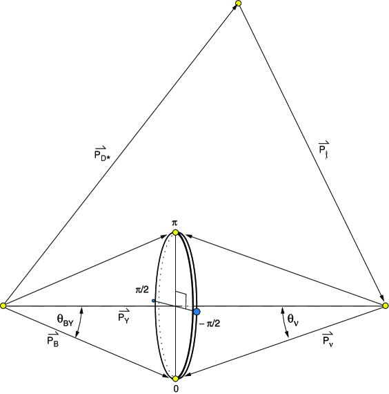
Figure 3: Diagram of $\cos\theta_{BY}$ reconstruction. The points at $\phi_{BY}=0$ and $\pi$ are in the $D^{*}-\ell$ plane. The points at $\pm\pi/2$ are out of the plane.

4.2 Kinematic variable determination

Without the neutrino we do not have sufficient information to fully reconstruct the kinematic variables $w$, ${\cos\theta_{\ell}}$, $\cos\theta_{V}$ and $\chi$. However, we can use the measured variables to construct an adequate approximation. Using energy-momentum conservation and assuming that the neutrino mass $m_{\nu}$ is zero, we have

$$0=m^{2}_{\nu}=M_{B}^{2}+M_{Y}^{2}-2E_{B}E_{Y}+2\wp_{B}\wp_{Y}\cos\theta_{BY},$$ (25)

where $p_{Y}=p_{D}^{*}+p_{\ell}$ is the four momentum of the combined $D^{*}$ and lepton, $M_{Y}^{2}=p_{Y}^{2}$ is the mass squared and $\wp_{Y}$ is the three-momentum. The $B$ meson energy $E_{B}$ and three-momentum $\wp_{B}$ can be estimated from the energies of the colliding beam particles, so we can solve for $\cos\theta_{BY}$ as follows

$$\cos\theta_{BY}=-\frac{M_{B}^{2}+M_{Y}^{2}-2E_{B}E_{Y}}{2\wp_{B}\wp_{Y}}.$$ (26)

Thus we can determine the angle between the $B$ and the direction ($\hat{Y}=\vec{p}_{Y}/\wp_{Y}$) of the $D^{*}-\ell$ system, but we do not know its azimuthal angle $\phi_{BY}$ around this direction. This is illustrated in Fig. 3. The direction of the $B$ must lie on the cone around $\hat{Y}$ defined by the angle $\theta_{BY}$.

For each possible $\phi_{BY}$ we can compute the kinematic variables $w$, ${\cos\theta_{\ell}}$, ${\cos\theta_{V}}$, $\chi$. Since we do not know which direction is correct we perform an average to estimate each variable. We average over four points: two in the $D^{*}$-lepton plane corresponding to the azimuthal angles $\phi_{BY}=0$ and $\pi$ and two points out of the plane corresponding to the angles $\pm\pi/2$. Further, since $B\bar{B}$ production follows a $\sin^{2}\theta_{B}$ distribution in the angle between the $B$ direction and the beam collision axis, we weight the kinematic variables evaluated at each point by the value $\sin^{2}\theta_{B}$ corresponding to the $B$ direction for that point.

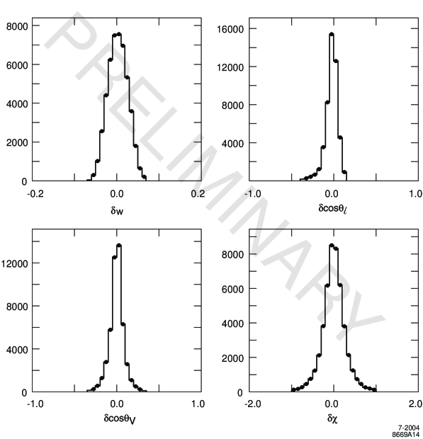
Figure 4: MC assessment of the experimental resolution for the variables $w$, ${\cos\theta_{\ell}}$, ${\cos\theta_{V}}$ and $\chi$. For each variable we plot the difference beween reconstructed and generated values. The resolution is generally small compared to the ranges of the variables as shown in Fig. 5.

Fig. 4 illustrates the resolution achieved by this ‘partial reconstruction’ technique. It is seen that the core widths for each resolution distribution are relatively small compared to the full width of each kinematic variable. The resolution is dominated by the average over the $B$ direction; detector resolution makes only a relatively minor contribution. The low-side tail on ${\cos\theta_{\ell}}$ can be attributed to final state radiation.

The resolutions of the four kinematic variables are highly correlated. A simple factorized resolution function in which the resolution is represented by a product of independent function for each variable fails to capture these correrlations. Thus, we are dependent on the Monte Carlo simulation to account for resolution effects.

The distributions of the reconstructed kinematic variables $w$, ${\cos\theta_{\ell}}$, ${\cos\theta_{V}}$ and $\chi$ are displayed in Fig. 5. The shaded region is the distribution of the background as estimated from the MC simulation using the method described in Sec. 6 below. It can be observed that the background distribution is much smaller than the signal contribution.

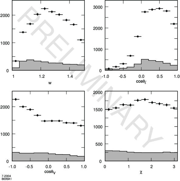
Figure 5: Distribution of kinematic variables $w$, ${\cos\theta_{\ell}}$, ${\cos\theta_{V}}$ and $\chi$ for selected events with estimated backgrounds (shaded region).

5 Simulation

This analysis is dependent on Monte Carlo (MC) simulation to model the efficiency and the background distributions. The degree to which we can trust our simulation to model both the detector and the underlying physics processes largely determines our systematic errors.

For the detector simulation we use BABAR’s GEANT4 based simulation [9]. The simulation has been validated and sophisticated correction procedures have been developed using many control samples. For simplicity, we do not apply these correction factors, but use them to evaluate systematic errors (which turn out to be small for this analysis, thereby justifying using them for a posteriori error estimation rather than as correction factors). Event generation and particle decay are modeled using the package EvtGen [10].

Figure 6: Distributions of the cosine of the helicity angle $\cos\theta_{V}$ for data (points) and MC (histogram) in bins of $D^{*}$ center-of-mass momentum. The momentum range for each plot is given its upper left-hand corner. The MC has been fit to the data as described in the text.

5.1 Slow pions

Of particular importance to this analysis is the modeling of the efficiency for detecting low-momentum pions. This is a difficult task since low momentum pions are lost through the interplay of acceptance, decay-in-flight, and stopping and scattering in the beam pipe or vertex detector. The performance of our simulation can be seen in Fig. 6, which shows the distribution of cosine of the helicity angle ($\cos\theta_{V}$) for $D^{*+}\rightarrow D^{0}\pi^{+}$ obtained from inclusively produced $D^{*}$ mesons for both the data and the MC sample in bins of center-of-mass momentum. The MC sample has been corrected by a factor of the form

$$f_{corr}=N\left(1+\alpha\cos\theta_{V}+\delta\cos^{2}\theta_{V})\right)$$ (27)

where the normalization and the parameters $\alpha$ and $\delta$ have been obtained from a fit to the data. The three lowest momentum bins are most relevant to $D^{*}\ell\nu$. The excellent agreement between the corrected MC and the data can clearly be observed in this figure.

The quadratic terms ($\delta$) may arise from differences in $D^{*}$ polarization; they are large ($\sim 0.5$ and $0.7$) in bins 2 and 3 where we expect the $D^{*}$ spectrum to be dominated by highly polarized few-body $B$ meson decays. The linear terms can only be attributed to differences in efficiency. The linear terms for the first three bins are small; i.e., they are $0.037\pm 0.16$, $-0.023\pm 0.024$ and $-0.016\pm 0.009$.

5.2 Final state radiation

The program PHOTOS [16] is used to model the effects of final state radiation (FSR). PHOTOS uses QED to second order in $\alpha_{em}$ (up to two FSR photons can be produced) and is known to provide an accurate simulation of the FSR effects.

5.3 Signal

To simulate the signal we use Eq. (2.2.1) for the distribution of the decay products. The MC samples are generated with the default parameters $R_{1}=1.180$, $R_{2}=0.720$ and ${\mbox{$\rho^{2}$}}=0.920$ [15].

5.4 Other semileptonic decays

A major source of background is other semileptonic $B$ decays. Aside from branching fractions for the decay modes $D\ell\nu$ and the signal mode $D^{*}\ell\nu$, only that for the mode $B\mbox{$\rightarrow$}D_{1}\ell\nu$ has been measured [11]. Thus, the other branching fractions used in the MC simulation are based on theory. Until such time as we can measure them, we must accept quite large possible variations in their numerical input values in our simulation.

6 Analysis Method

6.1 Fitting

Our basic approach to extracting the $D^{*}\ell\nu$ form factors is to perform an unbinned maximum likelihood fit to the full four-dimensional (4D) distribution (usually referred to as the probability density function or PDF in the context of likelihood fitting) specified by Eq. (2.2.1). We parameterize the form factors in terms of the HQET inspired parameters $R_{1}$, $R_{2}$ and $\rho^{2}$ as described in Sec. 2. Since theoretical predictions differ on the $w$ dependence of $R_{1}$ and $R_{2}$ (see Eqs.(17-23) ), we first give as our baseline result the values obtained by treating them as parameters which are constants over the entire range of $w$ (i.e. setting the coefficients of the $(w-1)$ and $(w-1)^{2}$ terms to zero and fitting only for the constant terms). This simplifies comparisons between experiments. However, we also show how the results vary when using the $w$-dependencies suggested by the full predictions of Eqs. (17-23).

In addition to assuming the form of the theoretical PDF, we must account for the effects of resolution and efficiency on the kinematic variable distribution. As our Monte Carlo samples are limited in size and do not allow us to adequately map the resolution and efficiency as a function of $w$, ${\cos\theta_{\ell}}$, ${\cos\theta_{V}}$ and $\chi$, we resort to the approximations derived below to allow us to correct for the effect of efficiency and resolution on the fitted parameters using only integrals of this efficiency. We must also account for the residual background.

To account for the efficiency and resolution effects we adapt the approach first employed in our angular analysis of the decay $B\rightarrow J/\psi K^{*}$[12] (for more details see also [14]). The PDF including resolution and efficiency ($\tilde{F}$) is given by

$$\tilde{F}(\tilde{x};\mu)=\int{dx\,\varepsilon(x)\,G(\tilde{x};x)\,F(x;\mu)}$$ (28)

where $x$ represents the true variables ($w$, ${\cos\theta_{\ell}}$, ${\cos\theta_{V}}$ and $\chi$), $\tilde{x}$ are the observed values of the variables and $\mu$ represents the parameters ($R_{1}$, $R_{2}$ and $\rho^{2}$) that determine the form factors. The efficiency $\varepsilon(x)$ is the fraction of events with parameters $x$ that will be – on average – detected and $G(\tilde{x};x)$ is the probability that an event with true parameters $x$ will be reconstructed with parameters $\tilde{x}$.

The log of the likelihood $L$ that we need to maximize is given by

$$\ln L=\sum_{i}{\ln\left(\frac{\tilde{F}(\tilde{x}_{i};\mu)}{N(\mu)}\right)}=\sum{\ln\tilde{F}(\tilde{x}_{i};\mu)}-N_{\rm signal}\times\ln N(\mu)$$ (29)

where the integral $N(\mu)\equiv\int{d\tilde{x}\tilde{F}(\tilde{x};\mu)}$ is needed to properly normalize the likelihood in the presence of imperfect acceptance. The sum is over our data event sample. $N_{\rm signal}$ is the number of signal events in the data sample.

Now consider the following trivial modification (multiplication by $1=F(x;\mu_{\rm mc})/F(x;\mu_{\rm mc}))$, where $\mu_{\rm mc}$ is the parameter set used to generate our Monte Carlo sample) of Eq. (28)

$$\tilde{F}(\tilde{x};\mu)=\int{dx\,\varepsilon(x)\,G(\tilde{x};x)\,F(x;\mu_{\rm mc})\times\frac{F(x;\mu)}{F(x;\mu_{\rm mc})}}$$ (30)

If $\mu$ is not too different from $\mu_{\rm mc}$ then the ratio $F(x;\mu)/F(x;\mu_{\rm mc})$ will not vary much across the range where the resolution function is much different from zero. In this case we can use $\tilde{x}$ to approximate $x$, which allows us to pull this ratio out of the integral to obtain

$$\widetilde{F}(\tilde{x};\mu)\approx\frac{F(\tilde{x};\mu)}{F(\tilde{x};\mu_{\rm mc})}\int{dx\,\varepsilon(x)G(\tilde{x};x)F(x;\mu_{\rm mc})}=F(\tilde{x};\mu)\frac{\tilde{F}(\tilde{x};\mu_{\rm mc})}{F(\tilde{x};\mu_{\rm mc})}.$$ (31)

When substituted into the expression for the log-likelihood this gives

$$\ln L=\sum\ln F(\tilde{x}_{i};\mu)-\sum\ln F(\tilde{x}_{i};\mu_{\rm mc})+\sum\ln\tilde{F}(\tilde{x}_{i};\mu_{\rm mc})-N_{\rm signal}\ln N(\mu).$$ (32)

Since terms that are independent of the fit parameters (constant terms) do not affect the point at which the maximum will be found, all the sums that depend on $\mu_{\rm mc}$ can be dropped. The $\mu$-dependent piece has been factored from these constant terms. We are left with a likelihood that depends only on the theoretical PDF $F$ and on the integral over the resolution and efficiency functions. Thus, there is no need for a detailed understanding of the efficiency and resolution as a function of the kinematic variables. All we need is a method for evaluating of the normalization integral $N(\mu)$

We can use the technique of Monte Carlo integration to evaluate the integral $N(\mu)$. We have

$$N(\mu)\approx\int{d\tilde{x}\tilde{F}(\tilde{x};\mu_{\rm mc})\times\frac{F(\tilde{x};\mu)}{F(\tilde{x};\mu_{\rm mc})}}\approx\frac{1}{N_{\rm gen}}\sum_{i}{\frac{F(\tilde{x}_{i};\mu)}{F(\tilde{x}_{i};\mu_{\rm mc})}}$$ (33)

where we have used the fact that the Monte Carlo generates events proportional to $\tilde{F}(\tilde{x};\mu_{\rm mc})$ to approximate the integral by a sum over MC events divided by the number of events generated, $N_{\rm gen}$.

We call this technique the ‘resolution-efficiency correction’ (REC) method. It can be shown to account for both the biases produced by resolution and efficiency if the Monte Carlo sample used was generated with parameters sufficiently near the final fitted values. As will be seen in the next section the small residual bias is also correctable.

The last remaining step is to handle the background. Ordinarily, we would add a PDF $B(\tilde{x})$ that models the background. The PDF $\tilde{F}$ would be replaced with

$$f\tilde{F}(\tilde{x};\mu)+(1-f)B(\tilde{x})$$ (34)

where $f$ is the signal fraction. However, since we do not have a form for the background before acceptance, we can not achieve the factorization of the parameter dependence from the efficiency and resolution functions that leads to Eq. (32). To avoid this problem we subtract the background directly in our likelihood sum rather than adding it to our PDF. We replace our log-likelihood function with the following ‘pseudo-likelihood’

$$\ln\mathchar 28931\relax=\sum_{i}\ln F(x^{(i)}_{\rm data};\mu)-\sum_{i}w^{(i)}_{\rm bkgd}\ln F(x^{(i)}_{\rm bkgd};\mu)-N_{\rm signal}\ln N(\mu))$$ (35)

where the first sum is over the data and the second is over a Monte Carlo sample representive of the background. This method is not as statistically optimal as using a proper likelihood – however, it is still unbiased.

The weights $w^{(i)}_{\rm bkgd}$ account for the normalization difference between the background in the data and in the Monte Carlo. They are computed in the manner indicated by Eqs. (41) and (42) in Sec. 6.2 below. We call this technique for handling the background the ‘direct unbinned background subtraction’ (DUBS) method.

The last term in Eq. (35) involves a sum (Eq. (33)) over the Monte Carlo data sample. This could be quite computationally intensive. However, we are able to speed up this computation by transforming the sum over events into a sum over ‘moments.’

Since our PDF can be written in the following form,

$$F(\tilde{x};\mu)=\sum_{\alpha}{A_{\alpha}(\mu)\times\mathchar 28932\relax_{\alpha}(x)},$$ (36)

i.e., as sum over a product of terms depending only on the fit parameters and terms depending only on the kinematic variables, we can define moments $M_{\alpha}$ by

$$M_{\alpha}=\frac{1}{N_{gen}}\sum_{i}{\frac{\mathchar 28932\relax_{\alpha}(\tilde{x}_{i})}{F(\tilde{x}_{;}\mu_{\rm mc})}}$$ (37)

where the sum is over reconstructed MC events, i.e., the same sum that defines $N(\mu)$ in Eq. (33). This allows us to write $N(\mu)$ as a sum over moments:

$$N(\mu)=\sum_{\alpha}{A_{\alpha}(\mu)\times M_{\alpha}}.$$ (38)

The moments can be computed once before fitting. In the fit, the time consuming event sum is replaced with the sum over moments. In our case taking the expansion of $h_{A_{1}}$ to order $(w-1)^{2}$ we have 18 moments to compute and sum.

6.2 Corrections and errors

The approximations outlined above (the REC and DUBS methods) provide us with a fast and easily implemented fitting procedure that uses the MC sample without any need to extract a detailed model of the efficiency and resolution functions. However, these advantages do not come without a price: we must make corrections for the small residual bias and we must account for the uncertainty introduced by the REC and DUBS procedures.

The REC method would be unbiased if the parameters $\mu_{\rm mc}$ used to generate the Monte Carlo sample turned out to be the same as the true parameters. This is, of course, in practice almost never the case, so we must ex post facto introduce a small correction. To do this we need the derivatives of the fitted parameters with respect to the input parameters. We obtain these by reweighting the Monte Carlo sample to correspond to parameters that deviate by $\pm 0.1$ from the parameters used in generation ($R_{1}=1.18$, $R_{2}=0.72$, $\rho^{2}=0.92$) and observing the differences produced in the fitted parameters. This yields the full $3\times 3$ matrix of the derivatives $d\mu_{\rm fitted}/d\mu_{\rm true}$.

Given the derivative matrix we can relate the results of our fit to the corrected results ($\mu_{\rm corrected}$) as follows

$$(\mu_{\rm fitted}-\mu_{\rm mc})_{=}\frac{d\mu_{\rm fitted}}{d\mu_{\rm true}}\times(\mu_{\rm corrected}-\mu_{\rm mc}).$$ (39)

To solve for the corrected parameters we need only invert the derivative matrix and multiply it against the LHS. The size of this correction is $\sim 0.05$ for $R_{1}$, $\sim 0.07$ for $R_{2}$ and $\sim-0.04$ for $\rho^{2}$.

Now since we use the theoretical PDF in our fit without explicit smearing to account for resolution, we have also underestimated the error. While the REC method corrects the values of the parameters for resolution effects (to a first approximation), it does not account for the loss of resolution due to our imperfect estimates of the four kinematic variables (which arise largely from not being able to obtain the exact $B$ rest frame, due to the missing neutrino, but also from detector smearing). However, the error matrix $E_{\rm fitted}$ for $R_{1}$, $R_{2}$ and $\rho^{2}$ can be corrected using the derivative matrix, as follows

$$E_{\rm fitted}\longrightarrow\left(\frac{d\mu_{\rm fitted}}{d\mu_{\rm true}}\right)^{-1}E_{\rm fitted}\left(\left(\frac{d\mu_{\rm fitted}}{d\mu_{\rm true}}\right)^{-1}\right)^{\dagger}.$$ (40)

This increases the error estimates by $\sim 12\%$.

We call this the ‘bias map correction’ (BMC) procedure, which refers to both the modifications of the central values, and to increase in the estimated statistical uncertainty.

In addition to the BMC error increase, there are contributions to the error that are not accounted for in the fit. Two of these are Monte Carlo statistical in nature: the error from the DUBS subtraction and the error from the Monte Carlo integration used to evaluate $N(\mu)$ in the REC procedure. There is also a contribution to the statistical error from the fluctuations in the background that is not accounted for in the fit. The first two can be reduced by increasing the size of the Monte Carlo sample, but the latter error is irreducible and must be included regardless of the size of the Monte Carlo sample.

We have developed procedures for evaluating these three errors using appropriate sums of the derivatives of the likelihood that can be evaluated using the Monte Carlo sample. The formulas used are collected in Appendix A.

6.3 Background

We rely on Monte Carlo to model the background. However, in order to subtract the background it must be properly normalized. To do this we adopt the background estimates from our $V_{cb}$ analysis [8]. The $V_{cb}$ analysis estimates the background by fitting the $\cos\theta_{BY}$ and $\delta m$ distributions. The $V_{cb}$ analysis fits the $\cos\theta_{BY}$ distributions for seven different background contributions (obtained either from MC or data sidebands, see [8] for a description of the seven categories). For our purposes we lump the background into two categories – peaking (candidates that contain a properly reconstructed $D^{*}$ and hence peak in the $\delta m$ distribution) and combinatoric (candidates in which the $D^{*}$ is a fake made from an incorrect combination of particles). Combinatorial is one of the seven categories above; we obtain the peaking fraction by summing over the other six.

The fractions of peaking and combinatorial background are determined in ten $w$-bins. Thus, we do not rely on the MC to model the $w$-dependence of the background, but take it from data.

For each $w$-bin we compute weights to apply to each event from the MC background sample before subtracting it. For the peaking component the weight for event $i$ is

$$w^{(i)}_{\rm peaking}=f_{\rm peaking}(w)\times N_{\rm data}\times\frac{w_{i}}{\sum w_{k}}$$ (41)

where the $w_{i}$ are weights we apply to correct for difference in the numbers of $B^{0}\bar{B}^{0}$, $B^{+}B^{-}$ and continuum Monte Carlo events available and $N_{\rm data}$ is the number of events in our signal window. The sum is over peaking background events ($k$) that are in the $w$-bin where the $w$ of the candidate falls.

This procedure guarantees that the number of peaking background events subtracted will be equivalent to the number ($f_{\rm peaking}(w)\times N_{\rm data}$) estimated to be inside the signal window.

A similar prescription applies for the combinatoric background with weights defined by

$$w^{(i)}_{\rm comb}=f_{\rm comb}(w)\times N_{\rm data}\times\frac{w_{i}}{\sum w_{k}}$$ (42)

where the events $k$ are now selected from the combinatoric category.

7 Results

For the baseline result we perform the fit taking $R_{1}$ and $R_{2}$ to be independent of $w$. All results are preliminary.

We find

$${\mbox{$R_{1}$}}=1.328\pm 0.055\pm 0.025$$

$${\mbox{$R_{2}$}}=0.920\pm 0.044\pm 0.020$$ (43)

$${\mbox{$\rho^{2}$}}=0.769\pm 0.039\pm 0.019$$

where the first error is statistical and the second Monte Carlo statistical. The BMC (Eqns.(39-40)) has been applied to both the central values and the the statistical error (it shifts the former and expands the latter). Systematic uncertainties are discussed in Sec. 9 below.

The errors are highly correlated. The error matrix for the full statistical error for $R_{1}$, $R_{2}$, and $\rho^{2}$ (including Monte Carlo) is:

                             0.003664   -0.001696    0.001213
                            -0.001696    0.002342   -0.001634
                             0.001213   -0.001634    0.001850

The correlations are

$$\rho_{R_{1}-R_{2}}=-0.58$$

$$\rho_{R_{1}-\rho^{2}}=+0.47$$ (44)

$$\rho_{R_{2}-\rho^{2}}=-0.79.$$

As we do not yet have enough sensitivity to fit for $w$-dependence of $R_{1}(w)$ and $R_{2}(w)$, we consider instead the effect of the theoretically predicted dependence on the result. Parameterizing this dependence as follows

$$R_{1}(w)=R_{1}+\alpha_{1}(w-1)+\beta_{1}(w-1)^{2}$$ (45)

$$R_{2}(w)=R_{2}+\alpha_{2}(w-1)+\beta_{2}(w-1)^{2}$$ (46)

and inserting these $w$-dependent forms into the PDF (with fixed $\alpha_{i},\beta_{i}$ from the theoretical predictions) and fitting for the constant terms $R_{1}$ and $R_{2}$  we find the results given in Table 1.

Table 1: Dependence of form factor parameters on theoretical assumptions about slope ($\alpha$) and curvature ($\beta$) of $R_{1}$ and $R_{2}$ $w$-dependence. See Eqns. (45) and (46).

Reference	$\alpha_{1}$	$\beta_{1}$	$\alpha_{2}$	$\beta_{2}$	$R_{1}$	$R_{2}$	$\rho^{2}$
Neubert[1]	-0.22	0.09	0.15	-0.04	1.37	0.88	0.75
Caprini-Lellouch-Neubert[4]	-0.12	0.05	0.11	-0.06	1.35	0.89	0.76
Ligeti-Grinstein[5]	-0.10	0.0	0.09	0.0	1.35	0.89	0.75
Baseline	0.0	0.0	0.0	0.0	1.33	0.92	0.77

Taking into account these theoretical variations in $R_{1}(w)$ and $R_{2}(w)$ yields slightly larger values for $R_{1}$ and slightly smaller values for $R_{2}$. The prediction by Neubert produces more deviation than the more recent calculations.

8 Goodness-of-fit

As these results are obtained from a maximum likelihood fit, we need some method of assessing whether the results of the fit actually reproduce the distribution of the kinematic variables in the data. Since we do not have an explicit form for the acceptance-corrected PDF ($\tilde{F}$) of the four reconstructed variables $w$, ${\cos\theta_{\ell}}$, ${\cos\theta_{V}}$ and $\chi$, we reweight the MC sample to construct the distributions expected from our measured parameters. That is, the contribution of the signal to a bin is

$$n_{\rm signal}=\sum{w^{(i)}_{\rm signal}}$$ (47)

where

$$w^{(i)}_{\rm signal}=\left(1-f_{\rm peaking}(w)-f_{\rm signal}(w)\right)\times N_{\rm data}\times\frac{w_{i}}{\sum w_{i}}$$ (48)

and in this case $w_{i}=\frac{F(x;\mu)}{F(x;\mu_{mc})}$ is the weight needed to modify the distributions from those generated with $\mu_{mc}$ ($R_{1}=1.18$, $R_{2}=0.72$, and $\rho^{2}=0.92$), to those we obtain from this analysis.

For the background we use the same weighting procedure (see Eqs. (41) and (42)) used in the fit. Using these weighting procedures the normalizations of the data and reweighted distributions match by construction.

We consider two types of goodness of fit: (a) five one-dimensional distributions (the projections $w$, ${\cos\theta_{\ell}}$, ${\cos\theta_{V}}$, and $\chi$ plus the distribution of CM lepton momentum $p^{*}_{\ell}$) and (b) a binned $\chi^{2}$ based on $6\times 6\times 6\times 6$ (a total 1296) bins. For a comparison we also give the unweighted results which corresponds closely to those using the CLEO parameters [2].

In Figs. 7-9 a comparison of the projections in the kinematic variables and $p^{*}_{\ell}$ between the Monte Carlo and the data can be seen. The plots in Fig. 7 show the result for the default parameters, while those in Fig. 8 give that obtained by reweighting by our parameters, and Fig. 9 shows both for the $p^{*}_{\ell}$ spectrum. The fit is to a constant from which we read off the $\chi^{2}$.

Close inspection will reveal that the ratio plot projections in Fig. 8 show better agreement to the line at unity than those in Fig. 7, but the improvement is more clearly seen numerically in Table 2, which gives the $\chi^{2}$ for fitting each plot to a constant. The constant is always consistent with unity as it must be. In every case the agreement between MC and data improves when we use our result – sometimes substantially.

Table 2: $\chi^{2}$ and $\chi^{2}$-probability for kinematic variable projections and lepton momentum; the number of bins in these histograms is 10. The number of degrees-of-freedom is 9, since we have forced the normalization.

variable	$\chi^{2}$ (prob.) default	$\chi^{2}$ (prob.) BaBar
$w$	14.08 (0.120)	13.69 (0.134)
${\cos\theta_{\ell}}$	17.12 (0.047)	7.626 (0.572)
${\cos\theta_{V}}$	40.93 (0.000)	17.81 (0.0374)
$\chi$	8.133 (0.521)	7.082 (0.623)
$p^{*}_{\ell}$	17.88 (0.037)	7.316 (0.604)

The value of the four-dimensional binned $\chi^{2}$ goes from $1274.04$ with default MC parameters to $1232.23$ with our parameters – an improvement of $\sim$$42$ units of $\chi^{2}$. The $\chi^{2}$ per bin is slightly smaller than unity. It is not really proper to interpret this as a probability as there are about 200 empty bins which contribute nothing to $\chi^{2}$. Nonetheless it is clear that the reweighted MC follows the distribution of the data quite well and that it models this decay (the single largest $B$ branching fraction) much better than the default MC.

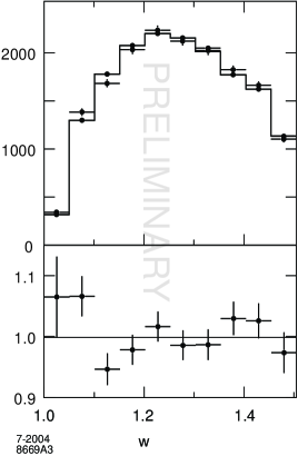
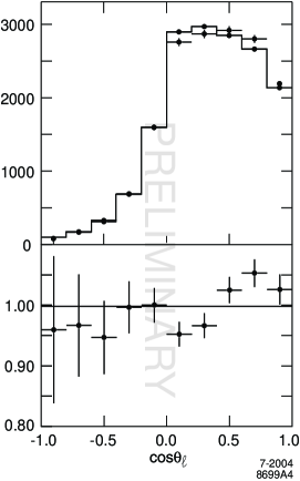
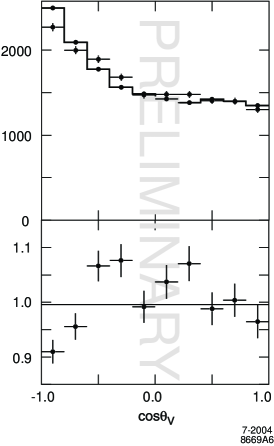
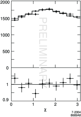
Figure 7: Data (points) overlayed on Monte Carlo (histograms) for all four kinematic variable distributions for default values of the parameters The plots below the overlays are the ratios of the data to MC distributions.

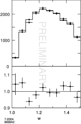
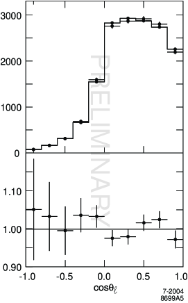
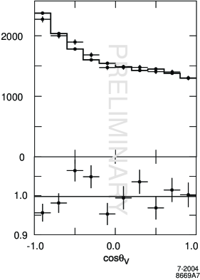
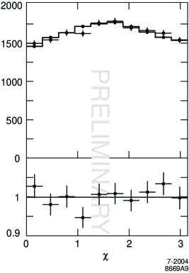
Figure 8: Data (points) overlayed on Monte Carlo (histogram) for all four kinematic variable distributions use our measurement of the parameters The plots below the overlays are the ratio of the data to the MC distributions.

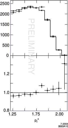
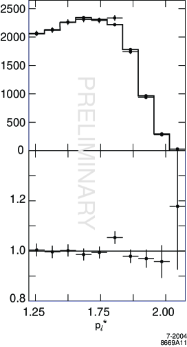
Figure 9: Data/Monte Carlo comparison for $p^{*}_{\ell}$-distribution (data are points, histograms are MC). MC used for the top plot uses default parameters and MC used for the bottom is reweighted to our parameters.

9 Systematic Studies

The systematic uncertainties on the three principal parameters are summarized in Table 5. The dominant systematic errors arise from the MC simulation: that is, from how well we understand and simulate the detector performance in terms of resolution and efficiencies, in particular the efficiency for the reconstruction of low-momentum charged pions from $D^{*+}$ decays. Further, how well we model the signal and background event generation, e.g. how close the branching fractions in the event generator are to those of the real world, affects the distribution of background we subtract. The $w$-dependence of the background, however, is not taken from the MC but is measured in the data and the uncertainty in this measurement also contributes to the systematic errors.

9.1 Detector Simulation

Extensive studies of the simulation of the detector response, including careful examination of track reconstruction efficiencies and particle identification, have been performed using selected data control samples. Adjustments for known simulation deficiencies are used in investigating and evaluating the systematic errors. Form factor measurements are insensitive to overall normalization errors. Thus differences in the efficiencies that are independent of the fit variables do not affect the results, but variations of differences as a function of these variables are of concern.

To assess the uncertainties due to differences in shape rather than normalization we vary the dependence on the efficiency corrections, reprocess the MC samples, redo the fit to the data, and take the difference to the results obtained with the nominal MC simulation as an estimate of the systematic error on the parameters. This procedure is repeated for every source of systematic uncertainty. The individual uncertainties are added in quadrature to obtain the total systematic error.

9.1.1 Charged Particle Tracking

The difference between the tracking efficiency for electrons, and charged kaons and pions from $D$ decays decreases roughly linearly as a function of momentum. We vary this linear dependence on the particle momentum in the MC simulation and observe no significant change in the results. Consequently, we assign no error from this source.

9.1.2 Slow Pion Reconstruction

The efficiency for reconstructing the low-momentum charged pion ($\pi_{s}$) from $D^{*+}$ is a major source of systematic errors. Because of the small energy release in $D^{*}$ decays, this pion is emitted in the same direction as the parent $D^{*}$ and its momentum is less than 400 ${\mathrm{\,Me\kern-1.00006ptV\!/}c}$ in the laboratory frame. Since $w=E_{D^{*}}/m_{D^{*}}$ in the B rest frame, the $\pi_{s}$ momentum is correlated with $w$ and thus its momentum dependent efficiency impacts the measurement of $\rho^{2}$.

The uncertainty due to the low-momentum tracking efficiency is evaluated differently from other tracking errors because such low-momentum tracks do not traverse the whole drift chamber. Their detection and measurement depends mostly on the silicon vertex tracker. To study this efficiency as a function of $p_{\pi_{s}}$ we use a large set of $D^{*+}\rightarrow D^{0}\pi_{s}^{+}$ decays selected from hadronic events and measure the distributions of the helicity angle of $\pi_{s}^{+}$ ($\theta_{V})$ in the $D^{*+}$ rest frame as a function of the $D^{*+}$ momentum. Fig. 6 in Sec. 5 compares the $\cos\theta_{V}$ obtained for data and MC simulation. The small size of the linear contributions to the correction factors (Eqn. 27) is encouraging, but there is enough room in the error that we still need to include the $\pi_{s}$ efficiency in the systematic error.

We parameterize the effective $\pi_{s}$ efficiency as function of its momentum using the form

$$\varepsilon(p_{\pi_{s}})=\varepsilon_{\rm max}\left(1-\frac{1}{1-\beta(p_{\pi_{s}}-p_{0})}\right)$$ (49)

with $p_{0}$ being the threshold momentum and $\beta$ controling the rapidity with which the efficiency rises above threshold. For $p_{\pi_{s}}<p_{0}$ we set $\varepsilon$ to zero. We fit the data and MC helicity angle distributions for $\beta$, $p_{0}$ and the coefficient of the physically allowed $\cos^{2}\theta_{V}$ term to obtain efficiency functions for the data and the MC. The helicity method only determines the relative momentum dependence of the efficiency, so the normalization $\varepsilon_{max}$ must be determined separately. Since, normalization does not matter for this analysis we simply set it to unity.

To assess the systematic uncertainty due to the $\pi_{s}$ efficiency we weight the MC simulation by the ratio of data to MC functions and assign the observed shifts in the fitted values for $R_{1}$, $R_{2}$ and $\rho^{2}$ as systematic errors. Not unexpectedly, $\rho^{2}$ is most sensitive to this efficiency since it describes the shape of the $w$-distribution.

9.1.3 Charged Particle Identification (PID)

Using data and MC simulated control samples we have tabulated the difference in particle identification efficiency for data and MC. These tables provide the correction factors in bins of momentum and angle. Since this analysis is most sensitive to efficiency variations with momentum we average the tables over the angles to obtain corrections as a function of momentum. For electrons the correction factors vary from 0.991 to 1.008 over the momentum range from $1.2{\mathrm{\,Ge\kern-1.00006ptV\!/}c}$ to $2.5{\mathrm{\,Ge\kern-1.00006ptV\!/}c}$. We assess the impact of the uncertainty in these corrections by approximating their momentum dependence by linear functions and vary the sign of the small slope of these functions. The observed deviations from the default fit are $\Delta R_{1}=0.0064$, $\Delta R_{2}=0.0052$ and $\Delta{\mbox{$\rho^{2}$}}=-0.0016$ for the positive slope and -0.0032, -0.0031, +0.0009 for the negative slope. We take half of the difference as the systematic error from this source. Since the momentum dependence is not a monotonic function, this procedure overestimates the uncertainty.

For kaon identification we employ the same procedure. The observed variations are significantly smaller.

The probability of misidentifying charged hadrons, $\pi^{\pm}$, $K^{\pm}$, $p^{\pm}$, as electrons is very small, less than $0.2\%$ in the momentum range $1.2-2.5{\mathrm{\,Ge\kern-1.00006ptV\!/}c}$. Since a variation of the peaking background by 9% results in a very modest change in the fit results, and since the fraction of this background originating from hadrons misidentified as electrons is very small, we conclude that the uncertainty in the hadron misidentification rate should be negligible.

The misidentification rate of pions as kaons ranges from a few tenths of a percent to almost $5\%$. However, pion misidentification is well simulated by the MC and thus should have little impact on the fit results. Furthermore, the main consequence of pion misidentification is to increase the combinatorial background. Since we estimate the combinatorial background from a fit to the measured $\delta m$ distribution, we are not dependent on the MC to assess the size of this background. We conclude that the uncertainty in the pion misidentification rate has little impact on the fit results.

9.2 Event Simulation

9.2.1 Final State Radiation (FSR)

Final state radiation, primarily from electrons, lowers the momenta and to a lesser degree changes the angles of detected particles. Though a physics effect, FSR acts much like a resolution – it smears the kinematic variables. We simulate the emission spectrum of radiative photons using PHOTOS [16], so the REC method corrects for it, to the extent that PHOTOS models it correctly.

To test the sensitivity to FSR we evaluate the shifts in the fitted values of $R_{1}$, $R_{2}$ and $\rho^{2}$ between fits done with and without FSR corrections. We assume an uncertainty of 30% in the simulated photon emission and thus take $\sim 1/3$ of the observed shifts of $0.0129$, $0.067$ and $0.0039$ as an estimate of the systematic uncertainty.

9.2.2 Background Simulation

We divide the background sources into two categories: (1) peaking background for which the $D^{*}$ decay has been correctly reconstructed and which contributes to the peak in the $\delta m=m_{K\pi^{+}\pi^{-}}-m_{K\pi}$ distribution and (2) combinatoric background for which the $D^{*}$ has not been properly reconstructed and thus does not contribute to the peak in the $\delta m$ distribution.

Background mixture

Our modeling of the peaking and combinatorial background depends on the not very well known branching fractions for the mixture of semi-leptonic $B$ decay modes that make up the background. To estimate the uncertainty associated with these branching fractions, we vary their values and observe shifts in the fit parameters compared to the nominal values. In this process we keep the total background fractions as determined by the $\cos\theta_{BY}$ fit (see Sec. 6.2) unchanged. We vary most modes by $60\%$. For the measured mode $B\mbox{$\rightarrow$}D_{1}l\nu$ we vary only by the $\sim 30\%$ measurement error[11]. In the case of $D^{*}l\nu$ there are contributions from badly reconstructed signal events. We assume a $20\%$ uncertainty in the signal branching fraction to account for the large differences in the currently available measurements.

Table 3: Systematic errors due to the uncertainties in the branching fractions of semileptonic $B$ decay modes. The branching fractions listed are the default values used in the MC simulation. The isospin related modes of neutral and charged $B$ mesons are varied together by the factors indicated.

Decay Mode	MC branching fraction (%)	Variation (%)	$\sigma_{R_{1}}$	$\sigma_{R_{2}}$	$\sigma_{\rho^{2}}$
$B\mbox{$\rightarrow$}D^{*}\ell\nu$	5.6	20	0.00052	0.00044	0.00027
$B\mbox{$\rightarrow$}D\ell\nu$	2.10	20	0.0013	0.00037	0.0002
$B\mbox{$\rightarrow$}D_{0}\ell\nu$	0.20	60	0.00020	0.00026	0.00010
$B\mbox{$\rightarrow$}D_{1}\ell\nu$	0.56	30	0.0087	0.0.0024	0.0016
$B\mbox{$\rightarrow$}D^{\prime}_{1}\ell\nu$	0.37	60	0.012	0.0062	0.0044
$B\mbox{$\rightarrow$}D_{2}\ell\nu$	0.37	60	0.00095	0.0025	0.0017
$B\mbox{$\rightarrow$}D^{*}\pi\ell\nu$	0.30	60	0.0036	0.00087	0.00071
$B\mbox{$\rightarrow$}D\pi\ell\nu$	0.9	60	0.0022	0.00092	0.00061
$e^{+}e^{-}\rightarrow c\bar{c}$	NA	20	0.0011	0.00034	0.00040
Total			0.016	0.0073	0.0051

In Table 3 we list these branching ratio variations as well as the effect of varying the contribution from $\mbox{$e^{+}$}\mbox{$e^{-}$}\rightarrow c\bar{c}$ events. We take half of the observed variation in the fit parameters as an estimate for the systematic error.

The total error for the three fit parameters is obtained by adding the errors due to each contribution in quadrature. $R_{1}$ is the most sensitive to the mixture of decay modes of the background subtraction.

Dependence of the Background on $w$

The $w$-dependence of the background estimate is taken from $\cos\theta_{BY}$ fits performed for each bin in $w$ [8]. We fit the $w$-dependence of the peaking and the combinatorial backgrounds to a second order polynomial centered at the middle bin. We use these polynomials, $f_{\rm peaking}(w)$ and $f_{\rm comb}(w)$, to compute the weights (see Eqs. (41) and (42)) that normalize our background subtraction.

To estimate the error from the $w$-dependence we vary the slopes of $f_{\rm peaking}(w)$ and $f_{\rm comb}(w)$ polynomials by $\pm 1\sigma$ and refit for $R_{1}$, $R_{2}$ and $\rho^{2}$ with the altered background normalizations. We take half of the total variation from each background type as its contribution to the systematic error.

Total peaking and combinatoric background fractions

Another source of error is the uncertainty in the normalization of the peaking and combinatoric background fractions. To estimate this error we vary the fraction $f_{\rm peaking}$ by $\pm 12\%$ and $f_{\rm comb}$ by $\pm 15\%$. We have increased these uncertainties beyond the statistical uncertainites established by our $V_{cb}$ analysis [8] to account for slight differences between the way the analyses define backgrounds. For $f_{\rm peaking}$ this yields errors of 0.0186, 0.0075, 0.0014 for the three parameters, indicating that this is a significant error source for $R_{1}$. For $f_{\rm comb}$ we find error estimates of 0.0063, 0.0034, 0.0080.

MC/data side-band comparison

The distributions of the kinematic variables for MC and data agree well in the $\delta m$ sideband region used to estimate the combinatoric background. But since the combinatoric background comprises about a third of the total background under the peak, the small differences in the shapes of the distributions could introduce an error in the background subtraction process (when the MC is used to subtract the residual combinatoric background from the data, see Sec. 6.1). To estimate the impact of this effect, we first take the ratios of data to MC in the sideband region and then fit the distributions with polynomials with the result shown in Fig. 10.

We then use these functions one at a time to multiply the combinatoric background from MC before it is subtracted from the data to prepare the sample for fitting. We then carry through the fits and then take the differences in the form factors we obtain from these with the form factors we obtain from the fits with the unaltered background. This procedure yields the results shown in Table 4.

The differences we find are small. The largest is from using the function for ${w}$, from which we find $\Delta\rho^{2}$ $\sim 0.006$. Since in the end we take the $w$-dependence of the background from the data and the deviations due to weighting the angular distributions are very small, we add nothing to the systematic uncertainty from this check.

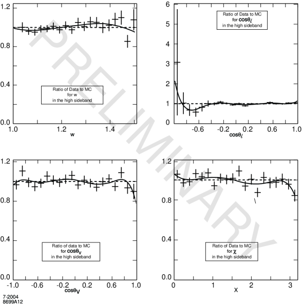
Figure 10: Ratio of data to MC for the four kinematic variables in the high sideband region  data, and the best polynomial fits.

Table 4: Changes in the fitted parameters for reweighting of the MC combinatoric background distributions in the four kinematic variables, as shown in Fig. 10.

Reweighted distributions	$R_{1}$	$R_{2}$	$\rho^{2}$
w distribution	-0.002	0.0	0.006
${\cos\theta_{\ell}}$ distribution	0.001	-0.002	-0.001
${\cos\theta_{V}}$ distribution	0.002	-0.003	0.001
${\chi}$ distribution	0.004	-0.002	0.001

9.3 Summary of Systematic Errors

The systematic errors are summarized in Table 5. While the total error remains statistics-dominated, we are approaching the systematic limit. The addition of other $D^{0}$ decay modes with higher multiplicity and higher backgrounds is likely to increase our sensitivity to the various background sources. Enhancing our understanding of these backgrounds will be critical to improving the errors. Measurements of the higher mass semileptonic decay modes are sorely needed.

Table 5: Summary of the estimated Systematic errors. Negligibly small contributions have been omitted here, they are discussed in the text: $D^{0}$ tracking, FSR, and $\delta m$ MC/data differences.

Error source	$\sigma_{{\mbox{$R_{1}$}}}$	$\sigma_{{\mbox{$R_{2}$}}}$	$\sigma_{{\mbox{$\rho^{2}$}}}$
Lepton-hadron track efficiency	0.005	0.004	0.002
Slow pion track efficiency	0.003	0.0002	0.011
PID misID (lepton, kaon)	0.005	0.004	0.002
Peaking background normalization	0.019	0.008	0.001
Combinatorial background normalization	0.006	0.003	0.008
Background composition (branching fractions)	0.016	0.0079	0.0051
$w$-dependence of background	0.001	0.001	0.028
Final state radiation	0.0043	0.0023	0.0013
Total Systematic	0.027	0.014	0.033

10 Conclusions

We have measured the form factors $A_{1}$, $V$ and $A_{2}$ in terms of the HQET-inspired parameters $R_{1}$, $R_{2}$ and $\rho^{2}$. Note that all results are preliminary.

The baseline result including systematic errors is

$$R_{1}=1.328\pm 0.055\pm 0.025\pm 0.025,$$ (50)

$$R_{2}=0.920\pm 0.044\pm 0.020\pm 0.013,$$

$$\rho^{2}=0.769\pm 0.039\pm 0.019\pm 0.032$$

where the first error is statistical, the second MC statistical, and the third systematic. This baseline result is obtained neglecting any possible $w$-dependence of $R_{1}(w)$ and $R_{2}(w)$. It agrees well, but not perfectly, with theory at $w=1$ (see eq. (17) or (20) ). We achieve a considerable improvement over the CLEO result of $R_{1}=1.18\pm 0.30\pm 0.12$, $R_{2}=0.71\pm 0.22\pm 0.07$ and $\rho^{2}=0.91\pm 0.15\pm 0.06$ [2].

We do not yet have the sensitivity to independently establish the $w$-dependence of $R_{1}(w)$ and $R_{2}(w)$, but we can use theoretical estimates to make comparisons. If we compare the predictions of Caprini, Lellouch and Neubert [4] for $R_{1}$ and $R_{2}$ to the result we obtain using their $w$-dependence (see Table 1), we find $\Delta R_{1}=1.36-1.27=0.09$ ($1.6\sigma$ statistical) and $\Delta R_{2}=0.87-0.80=0.07$ ($1.4\sigma$ statistical). Given the undoubted presence of theoretical errors, this is reasonable agreement.

This measurement allows us to make a considerable improvement in the size of the current error in $V_{cb}$ measurements. For our measurement of $V_{cb}$ the error contributed by uncertainty in $R_{1}$ and $R_{2}$ drops by a factor $\sim 4$ from that obtained using the previous measurement from CLEO [2]. The effect on the total uncertainty is to reduce it by $\sim 30\%$.

A considerable improvement can also be obtained in measurements of the lepton end point spectrum. The systematic error on the branching fraction for decays with a lepton in the momentum range $2.1-2.6{\mathrm{\,Ge\kern-1.00006ptV\!/}c}$ is reduced from $5\%$ to $1.7\%$ which corresponds to an improvement of $\sim 8\%$ in the total statistical plus systematic error.

In addition we have demonstrated useful approximations to the maximum likelihood method that allow us to cope with the limited size of the Monte Carlo samples available to modern high luminosity experiments. We have also developed the procedures needed to evaluate the corrections and additional uncertainties due to these approximations. These methods are not unique to $D^{*}\ell\nu$ or $J/\psi K^{*}$, but could be applied to any analysis that needs to cope with a complex multi-dimensional acceptance and resolution problem.

11 Acknowledgments

The authors wish to thank Z.Ligeti and M.Neubert for very useful discussions of the theoretical issues.

We are grateful for the extraordinary contributions of our PEP-II colleagues in achieving the excellent luminosity and machine conditions that have made this work possible. The success of this project also relies critically on the expertise and dedication of the computing organizations that support BABAR. The collaborating institutions wish to thank SLAC for its support and the kind hospitality extended to them. This work is supported by the US Department of Energy and National Science Foundation, the Natural Sciences and Engineering Research Council (Canada), Institute of High Energy Physics (China), the Commissariat à l’Energie Atomique and Institut National de Physique Nucléaire et de Physique des Particules (France), the Bundesministerium für Bildung und Forschung and Deutsche Forschungsgemeinschaft (Germany), the Istituto Nazionale di Fisica Nucleare (Italy), the Foundation for Fundamental Research on Matter (The Netherlands), the Research Council of Norway, the Ministry of Science and Technology of the Russian Federation, and the Particle Physics and Astronomy Research Council (United Kingdom). Individuals have received support from CONACyT (Mexico), the A. P. Sloan Foundation, the Research Corporation, and the Alexander von Humboldt Foundation.

Appendix A: Evaluation of additional errors

Here we gather the equations used to evaluate the errors not included in our likelihood fit. Specifically, we provide equations for the errors due to the Monte Carlo integration of the REC method, that due to the background subtraction of the DUBS method, and that due to the fluctuations of the actual background initially left unaccounted for when the DUBS method is used.

Full details and derivations can be found in the thesis of M.S. Gill[14].

REC Monte Carlo integration error

The REC Monte Carlo integration error is given by:

$$E_{rec}=E_{fit}DE^{\dagger}_{fit}$$ (51)

where $E_{fit}$ matrix is the error reported by the fitter. $D$ is a matrix of derivative sums.

$D$ is composed of three pieces. To lay them out we need to define some terms.

The sums of the weights $w_{i}\equiv F(\tilde{x}_{i};\mu)/F(\tilde{x}_{i};\mu_{mc})$ used in the integral:

$$W(\mu)=\sum{w_{i}}$$ (52)

where sums over MC events used to evaluate the normalization integral $N(\mu)$.

The vector of the derivatives weights:

$$\Delta_{i}\equiv\frac{dw_{i}}{d\mu}=\left(\frac{\partial w_{i}}{\partial R_{1}},\frac{\partial w_{i}}{\partial R_{2}},\frac{\partial w_{i}}{\partial{\mbox{$\rho^{2}$}}}\right)$$ (53)

where $F_{i}\equiv F(\tilde{x}_{i};\mu)$. The derivatives are computed numerically though an analytic compuation is possible.

The sum of weights squared:

$$W_{sq}(\mu)\equiv\sum w^{2}_{i}$$ (54)

The $W$ derivative vector:

$$\frac{dW}{d\mu}=\sum\Delta_{i}$$ (55)

which also allows us to compute $\frac{dLnW}{d\mu}=\frac{1}{W}\frac{dW}{d\mu}$.

Weight $\times$ derivative vector:

$$WdW=\sum w_{i}\times\Delta_{i}$$ (56)

Derivative $\times$ Derivative matrix:

$$dWdW=\sum\left(\Delta_{i}\Delta_{i}^{\dagger}\right)$$ (57)

The three components are give by:

$$D_{1}=\eta\times dWdW$$ (58)

$$D_{2}=-\eta\times W_{sq}\left(\left(\frac{dW}{d\mu}\right)\times\left(\frac{dW}{d\mu}\right)^{\dagger}\right)$$ (59)

$$D_{3}=-\eta\times\left(\left(\frac{dLnW}{d\mu}\right)WdW^{\dagger}+WdW\left(\frac{dLnW}{d\mu}\right)^{\dagger}\right)$$ (60)

where $\eta=N_{signal}/W^{2}$ is a normalization factor.

$D$ is just the sum of these three, i.e., $D=D_{1}+D_{2}+D_{3}$.

DUBS error

The DUBS error can be computed from sums over the Monte Carlo sample used in the background subtraction. In this case the weights ($w_{i}$) are those used to weight each type of background to obtain the correct normalization as described in Sec. 6.2 (see eqs. (41) (42)).

In this we need the vector of the derivatives of the PDF $\frac{dLnF_{i}}{d\mu}$ from which we compute the ‘sensitivity’ matrix $S$:

$$S_{dubs}=\sum w^{2}_{i}\left(\frac{dLnF_{i}}{d\mu}\right)\left(\frac{dLnF_{i}}{d\mu}\right)^{\dagger}$$ (61)

Given $S$ the DUBS error is just:

$$E_{dubs}=E_{fit}S_{dubs}E^{\dagger}_{fit}$$ (62)

Background error

We also use the DUBS sample to estimate error from background in our signal sample. The result is analogous to eq. (61) accept that $w^{2}_{i}$ is replaced by $w_{i}$. That is, we have:

$$S_{back}=\sum w_{i}\left(\frac{dLnF_{i}}{d\mu}\right)\left(\frac{dLnF_{i}}{d\mu}\right)^{\dagger}$$ (63)

and

$$E_{back}=E_{fit}S_{back}E^{\dagger}_{fit}$$ (64)

References

- [1] M. Neubert, “Heavy Quark Symmetry”, Physics Reports 259:245 (1994) [hep-ph/9306320].
- [2] J.E. Duboscq et.al. (CLEO Collab.), Phys. Rev. Lett. 76: 3898 (1996).
- [3] N. Isgur and M.B. Wise, Phys. Lett. B237:527 (1990).
- [4] I. Caprini, L. Lellouch, M. Neubert, Nucl.Phys. B530:153-181 (1998) [hep-ph/9712417].
- [5] B.Grinstein, Z.Ligeti, Phys.Lett. B526:345-354 (2002) [hep-ph/0111392].
- [6] F.Close, A. Wambach, Nucl.Phys. B412:169-180 (1994) [hep-ph/9307260].
- [7] The BABAR Collaboration, B. Aubert et al., Nucl. Instrum. Methods A479:1-116 (2002).
- [8] BABAR, paper, Submitted Paper, ICHEP 2004 Conference Proceedings [hep-ex/0308027]
- [9] S. Agostinelli et al., Geant4 Collaboration, Nucl. Instrum. Methods A506:250-302 (2003).
- [10] D. Lange et al., Nucl. Instrum. Methods A462:152-155 (2001).
- [11] Review of Particle Physics, K. Hagiwara et al., Phys. Rev. D66, 010001 (2002), [http://pdg.lbl.gov]
- [12] Measurement of the Decay Amplitudes. By the BABAR Collaboration, Phys.Rev.Lett.87:241801 (2001) [hep-ex/0107049].
- [13] BaBar, ICHEP Form Factor Paper Submission Long Version (2004) [http://www.slac.stanford.edu/\̃hbox{}msgill/FFdocs/ichepPaper.v11.ps]
- [14] M. S. Gill, Ph.D. Thesis, University of California, Berkeley (UCB), (2004) [http://www.slac.stanford.edu/\̃hbox{}msgill/FFdocs/ffthesis.ps]
- [15] A. Ryd, Ph.D. Thesis, University of California, Santa Barbara (UCSB), (1997).
- [16] S. Jadach, B. Ward, Z. Was, Comput.Phys.Commun.130:260-325 (2000).