Reweighting of the form factors in exclusive $B\rightarrow X\ell\nu_{\ell}$ decays

Abstract

A form factor reweighting technique has been elaborated to permit relatively easy comparisons between different form factor models applied to exclusive $B\rightarrow X\ell\nu_{\ell}$ decays. The software tool developped for this purpose is described. It can be used with any event generator, three of which were used in this work: ISGW2, PHSP and FLATQ2, a new powerful generator. The software tool allows an easy and reliable implementation of any form factor model. The tool has been fully validated with the ISGW2 form factor hypothesis. The results of our present studies indicate that the combined use of the FLATQ2 generator and the form factor reweighting tool should play a very important role in future exclusive $|V_{ub}|$ measurements, with largely reduced errors.

1 Introduction

Exclusive semileptonic $B\rightarrow X_{u}\ell\nu_{\ell}$ decays can be used to measure the magnitude of the CKM matrix element $V_{ub}$ as their branching fractions (B.F.) are related to $|V_{ub}|$ by the following relation:

$$|V_{ub}|=\sqrt{\frac{B.F.(B\rightarrow X_{u}\ell\nu_{\ell})}{x\cdot\tau_{B}}}$$ (1)

where $\tau_{B}$ is the lifetime of the $B$ meson and $x$ is given by the relation : $\Gamma_{th}(B\rightarrow X_{u}\ell\nu_{\ell})=x|V_{ub}|^{2}$, $\Gamma_{th}$ is the theoretical partial decay rate.

The study of exclusive semileptonic $B\rightarrow X_{u}\ell\nu_{\ell}$ decays offers some experimental advantages compared to an inclusive study of all $b\rightarrow u\ell\nu_{\ell}$ decays, such as the possibility of keeping a higher fraction of the phase space and permitting a better background rejection. On the other hand, it deals with lower statistics and it is affected by large theoretical uncertainties arising from the calculation of the form factors describing the strong interaction effects on the hadronization of the different $X_{u}$ final states. These uncertainties in the form factors lead to different predictions of the shape of the differential decay rate which, in turn, yield different predictions for the momentum spectrum of the lepton $\ell$, the meson $X_{u}$ and its daughters. The subsequent varying efficiencies for the experimental cuts lead to uncertainties in the measured branching fractions. The theoretical uncertainties in the form factors also affect the values of $x$. The resulting uncertainty in $x$ is the largest source of uncertainty in the determination of $|V_{ub}|$ from exclusive branching fraction measurements.

In addition, in many analyses (e.g. those performed in BaBar), the simulated inclusive lepton spectrum of B decays does not agree with data. Since the $B\rightarrow D\ell\nu_{\ell}$ and $B\rightarrow D^{*}\ell\nu_{\ell}$ are the most abundant of all $B$ decays, it is likely that at least part of the disagreement could arise from a wrong theoretical input to the simulation for these decays. Again, the most likely source of error comes from the form factors for these decays. Since the theoretical form factor predictions cover a rather large range, it is necessary to establish experimentally which theory best describes the data. This requires the possibility of varying the theoretical assumptions at the simulation level.

A tool to be described in this paper has been created for this purpose. It will permit to switch easily between various form factor hypotheses and/or to vary the parameters of a given hypothesis, within a full standard Geant4 Monte Carlo (MC) simulation framework. The basic principle of this new tool is to generate events and run the full simulation and reconstruction sequence only once, with a given form factor hypothesis. Subsequently, the events thus generated are reweighted at the ntuple level with the values provided by a different form factor hypothesis.

The relevant formulas and basic principles of the form factor reweighting technique are presented in Sect. 2. In Sect. 3, the structure of the software tool developped for this purpose and how to use it are described. In that section, we also show how to incorporate new form factor hypotheses in the tool. Several histograms that demonstrate that the tool is working properly are shown in Sect. 4. A sample of kinematical distributions calculated with different form factor models are compared in Sect. 5. The conclusions are given in Sect. 6.

2 Technique for form factors reweighting

2.1 Pseudo-scalar versus vector mesons

The exclusive $B\rightarrow X_{u}\ell^{+}\nu_{\ell}$ decays which could be studied with this technique are: $B^{+}\rightarrow\pi^{0}/\eta/\eta^{\prime}/\rho^{0}/\omega\ell^{+}\nu_{\ell}$ and $B^{0}\rightarrow\pi^{-}/\rho^{-}\ell^{+}\nu_{\ell}$. As will be shown in Sect. 2.4, the differential decay rates are different for pseudo-scalar and vector mesons. The $B^{0}$, $B^{\pm}$, $\pi^{\pm}$, $\pi^{0}$, $\eta$ and $\eta^{\prime}$ mesons are all pseudo-scalar particles, while the $\rho^{\pm}$, $\rho^{0}$ and $\omega$ mesons are vector particles. As well, the most abundant $B\rightarrow X_{c}\ell^{+}\nu_{\ell}$ decays, $B\rightarrow D\ell^{+}\nu_{\ell}$ and $B\rightarrow D^{*}\ell^{+}\nu_{\ell}$, involve $D$ pseudo-scalar mesons and $D^{*}$ vector mesons.

2.2 Kinematics of semileptonic decays

A semileptonic $B\rightarrow X\ell\nu$ decay is generally described by the following process. The $B$ meson first decays into a virtual $W^{\pm}$ boson and an $X$ meson which are emitted back to back in the $B$ frame. The virtual $W^{\pm}$ boson then decays to a lepton and a neutrino which are emitted back to back in the $W^{\pm}$ frame, while the $X$ meson decays in various ways. The kinematics of such semileptonic decays can be completely described by three angles: $\theta_{\ell}$, $\theta_{V}$ and $\chi$ defined in Fig. 1 and by $q^{2}$, the invariant mass squared of the virtual $W^{\pm}$ boson. In terms of 4-momenta:

$$q^{2}=(p_{\ell}+p_{\nu})^{2}=(p_{B}-p_{X})^{2}$$ (2)

The four variables are totally uncorrelated. In the $B$ frame, $q^{2}$ is also given by:

$$q^{2}=m_{B}^{2}+m_{X}^{2}-2m_{B}E_{X}$$ (3)

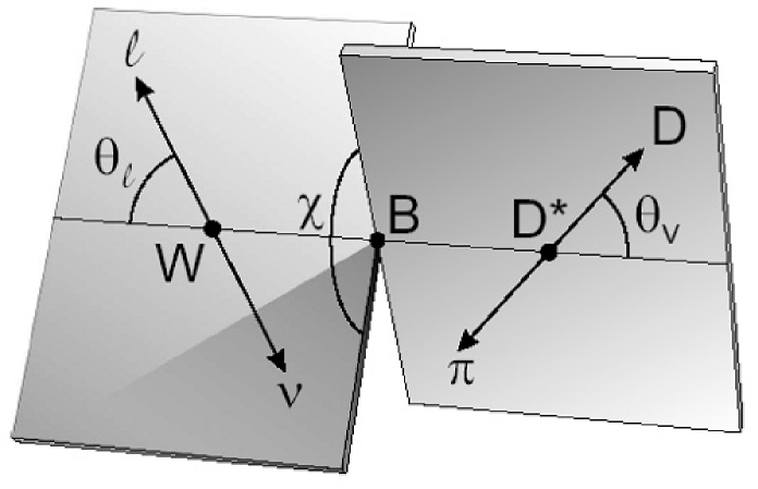
Figure 1: Definition of the angles $\theta_{\ell}$, $\theta_{V}$ and $\chi$ in the case of the $B$ to vector semileptonic decay $B\rightarrow D^{*}\ell\nu$, $D^{*}\rightarrow D\pi$. $\theta_{\ell}$ is the helicity angle of the $W^{\pm}$ boson, the angle between the direction of the $W$ boson boosted in the $B$ frame and the direction of the lepton boosted in the $W^{\pm}$ frame (where the $\ell$ and $\nu$ are emitted back to back). $\theta_{V}$ is the helicity angle of the X meson, here the angle between the direction of the $D^{*}$ meson boosted in the $B$ frame and the direction of the $D$ meson boosted in the $D^{*}$ frame (where the $D$ and $\pi$ mesons are emitted back to back). $\chi$ is the angle between the $\vec{W}\times\vec{\ell}$ plane and the $\vec{D^{*}}\times\vec{D}$ plane.

where $E_{X}$ is the total energy of the $X$ meson. It is also of interest to note that the magnitude of the 3-momentum $\vec{p_{X}}$ and $q^{2}$ are uniquely related by Eq. 4 in the $B$ frame:

$$|\vec{p_{X}}|=\sqrt{\frac{(m_{B}^{2}+m_{X}^{2}-q^{2})^{2}}{4m_{B}^{2}}-m_{X}^{2}}$$ (4)

2.3 Form factors

The matrix element of a semileptonic $B\rightarrow X\ell\nu_{\ell}$ decay can be written as BurchatRichman :

$$M(B\rightarrow X\ell\nu_{\ell})=-i\frac{G_{F}}{\sqrt{2}}V_{xb}L^{\mu}H_{\mu}$$ (5)

where $G_{F}$ is the weak interaction’s Fermi constant, $V_{xb}$ is either $V_{ub}$ or $V_{cb}$ depending on the final state meson, $L^{\mu}$ is the leptonic current and $H_{\mu}$ is the hadronic current. The leptonic current is well-known and can be calculated precisely using perturbation theory.

The hadronic current accounts for the strong interactions between quarks and gluons, and thus for the hadronization of the final state quarks into a X meson. The hadronization of a $\bar{u}$ quark and a $d$ spectator quark into a $\pi^{-}$ meson in a $B^{0}\rightarrow\pi^{-}\ell^{+}\nu_{\ell}$ decay is a good example of such a situation. In all these processes which involve the exchange of soft gluons, the strong interaction coupling constant, $\alpha_{s}(\mu)$, is too large to allow the use of perturbative calculation techniques. Thus, even though the structure of hadronic currents is well known, such currents cannot be computed directly. However, they can be parametrized in terms of a small number of so-called universal Isgur-Wise functions, or form factors isgw2 . To compute the form factors, it is necessary to use either non-perturbative calculation techniques such as lattice QCD FNAL01 , or approximations of QCD. The approximation techniques can themselves be split into two categories: 1) those, such as the Light Cone Sum Rules (LCSR) ball98 ball01 , which are identical to QCD at some extreme limits but are a good approximation of QCD in a restricted but known kinematic range and 2) those, such as ISGW2 isgw2 which, instead of QCD, use approximate wave functions based on quark models for the mesons. The values of the form factors extracted from experimental data can then be confronted with various models or used on their own.

In terms of form factors, the hadronic current is given by a different expression depending on whether the $B$ meson decays to a pseudo-scalar or to a vector meson final state. In both cases however, the expression for the hadronic current can be simplified in the limit BurchatRichman of a massless lepton, assumed to be true when $\ell=e$ or $\mu$ (see Sect. 4.4 for an estimate of the effect of this approximation).

For decays such as $\bar{B}^{0}\rightarrow\pi^{+}\ell^{-}\bar{\nu}_{\ell}$ where $\pi^{+}$ is a pseudo-scalar meson, the hadronic current is written, in the limit of a massless lepton as BurchatRichman :

$$H^{\mu}=\langle\pi^{+}(p^{\prime})|u\gamma^{\mu}b|\bar{B^{0}}(p)\rangle=f^{+}(q^{2})(p+p^{\prime})^{\mu}$$ (6)

where $q=p-p^{\prime}$ and $f^{+}(q^{2})$ is the form factor describing the non-perturbative QCD effect.

For decays such as $\bar{B}^{0}\rightarrow\rho^{+}\ell^{-}\bar{\nu}_{\ell}$ where $\rho^{+}$ is a vector meson, the hadronic current is written, in the limit of a massles lepton as BurchatRichman :

$$H^{\mu} = \langle\rho^{+}(p^{\prime},\epsilon)|u\gamma^{\mu}(1-\gamma_{5})b|\bar{B^{0}}(p)\rangle$$

$$= \frac{2i\epsilon^{\mu\nu\alpha\beta}}{m_{B}+m_{\rho}}\epsilon^{*}_{\nu}p^{\prime}_{\alpha}p_{\beta}V(q^{2})-(m_{B}+m_{\rho})\epsilon^{*\mu}A_{1}(q^{2})$$

$$+ \frac{\epsilon^{*}\cdot q}{m_{B}+m_{\rho}}(p+p^{\prime})^{\mu}A_{2}(q^{2})$$

where $A_{1}(q^{2})$, $A_{2}(q^{2})$ and $V(q^{2})$ are the three form factors describing the non-perturbative QCD effect.

The equations for these two hadronic currents as well as their expressions without the massless lepton approximation are discussed in various papers, for example in Ref. BurchatRichman .

It is important to note that the leptonic current and the structure of the hadronic currents (Eqs. 6 and 2.3) follow directly from Lorentz invariance and are thus model-independent. The theoretical uncertainties in exclusive semi-leptonic decay analyses are only due to the uncertainties in the knowledge of the form factor(s): $f^{+}(q^{2})$, $A_{1}(q^{2})$, $A_{2}(q^{2})$ and $V(q^{2})$ which are model-dependent. These factors nominally depend only on a single variable: $q^{2}$. However, in the case of vector meson decays, interference effects between the $A_{1}(q^{2})$, $A_{2}(q^{2})$ and $V(q^{2})$ form factors introduce an additional model dependence for the angular differential decay rates cote .

2.4 Differential decay rates

The differential and total decay rates are the observable manifestations of the underlying leptonic and hadronic currents. According to quantum field theory, the decay rate is given by a squared matrix element containing a combination of leptonic and hadronic currents. Just like for the structure of the current equations (Sect. 2.3), the structure of the differential and total decay rate equations is also considered to be model-independent. Only the form factors appearing in the rates give rise to theoretical uncertainties in exclusive semi-leptonic decay analyses cote . These will be investigated.

Our investigation will be greatly simplified by the use of a technique to reweight the form factors among the various hypotheses under study. As will be shown in Sect. 2.5, this reweighting is equivalent to a reweighting of the differential decay rates i.e. of the probabilities of generating an event. The total decay rate $\Gamma$ does have a large effect cote on the model dependency of $B\rightarrow X\ell\nu$ analyses but is not used in the context of form factor reweighting.

In the limit of a massless lepton, the differential decay rate of semileptonic B decays to a pseudo-scalar meson is given by BurchatRichman :

$$\frac{d\Gamma(B\rightarrow S\ell^{+}\nu_{\ell})}{dq^{2}d\cos\theta_{\ell}d\cos\theta_{V}d\chi}=|V_{xb}|^{2}\frac{G_{F}^{2}}{128\pi^{4}}|\vec{p_{S}}|^{3}\sin^{2}\theta_{\ell}\sin\theta_{V}|f^{+}(q^{2})|^{2}$$ (8)

where $q^{2}$, $\theta_{V}$, $\theta_{\ell}$ and $\chi$ have been defined in Sect. 2.2, $\vec{p_{S}}$ is the 3-momentum of the final state pseudo-scalar meson in the $B$ frame, $f^{+}(q^{2})$ is the QCD form factor described in Sect. 2.3 and $V_{xb}$ is either $V_{ub}$ or $V_{cb}$ depending on the final state meson. It is often practical to use an expression where two or three of the angles are integrated out in which case Eq. 8 becomes Gibbons :

$$\frac{d\Gamma(B\rightarrow S\ell^{+}\nu_{\ell})}{dq^{2}d\cos\theta_{\ell}}=|V_{xb}|^{2}\frac{G_{F}^{2}}{32\pi^{3}}|\vec{p_{S}}|^{3}\sin^{2}\theta_{\ell}|f^{+}(q^{2})|^{2}$$ (9)

$$\frac{d\Gamma(B\rightarrow S\ell^{+}\nu_{\ell})}{dq^{2}}=|V_{xb}|^{2}\frac{G_{F}^{2}}{24\pi^{3}}|\vec{p_{S}}|^{3}|f^{+}(q^{2})|^{2}$$ (10)

Also, in the limit of a masless lepton, the differential decay rate of semileptonic B decays to a vector meson is BurchatRichman :

$$\frac{d\Gamma(B\rightarrow V\ell^{+}\nu_{\ell})}{dq^{2}d\cos\theta_{\ell}d\cos\theta_{V}d\chi}=|V_{xb}|^{2}\frac{3G_{F}^{2}|\vec{p_{V}}|q^{2}}{8(4\pi)^{4}m_{B}^{2}}$$

$$\times \left\{\begin{array}[]{l}(1-\cos\theta_{\ell})^{2}\sin^{2}\theta_{V}|H_{+}(q^{2})|^{2}\\ +(1+\cos\theta_{\ell})^{2}\sin^{2}\theta_{V}|H_{-}(q^{2})|^{2}\\ +4\sin^{2}\theta_{\ell}\cos^{2}\theta_{V}|H_{0}(q^{2})|^{2}\\ -4\sin\theta_{\ell}(1-\cos\theta_{\ell})\sin\theta_{V}\cos\theta_{V}\cos\chi H_{+}(q^{2})H_{0}(q^{2})\\ +4\sin\theta_{\ell}(1+\cos\theta_{\ell})\sin\theta_{V}\cos\theta_{V}\cos\chi H_{-}(q^{2})H_{0}(q^{2})\\ -2\sin^{2}\theta_{\ell}\sin^{2}\theta_{V}\cos 2\chi H_{+}(q^{2})H_{-}(q^{2})\\ \end{array}\right\}$$

(12)

where $\vec{p}_{V}$ is now the 3-momentum of the final state vector meson in the $B$ frame. The functions $H_{+}(q^{2})$, $H_{-}(q^{2})$ and $H_{0}(q^{2})$ are known as the helicity amplitudes of the vector meson. They are related cote to the QCD form factors $A_{1}(q^{2})$, $A_{2}(q^{2})$ and $V(q^{2})$ described in Sect. 2.3. Integrating out the angles, Eq. 12 becomes:

$$\frac{d\Gamma(B\rightarrow V\ell^{+}\nu_{\ell})}{dq^{2}}=|V_{xb}|^{2}\frac{G_{F}^{2}|\vec{p_{V}}|q^{2}}{96\pi^{3}m_{B}^{2}}\times$$

$$\;\;\;\;\;\;\;\;\;\;\;\;\;\;\;\;\left(|H_{+}(q^{2})|^{2}+|H_{-}(q^{2})|^{2}+|H_{0}(q^{2})|^{2}\right)$$ (13)

As can be seen from Eqs. 8 and 12, the form factors introduce a model dependence in the prediction of the shape of the differential decay rates of both pseudo-scalar and vector meson decays. This will be shown explicitly in Sect. 5. With standard procedures, this theoretical uncertainty in the shape of the differential decay rate leads to a “theoretical” uncertainty in the efficiency of the experimental cuts, and thus on the measured branching fraction.

2.5 Reweighting the probabilities of generating events among various form factor models

A useful feature of the form factor reweighting tool is that events are generated, fully simulated and reconstructed only once, using a given form factor hypothesis. The probabilities of generating events are then reweighted to any other form factor model at the ntuple level. Such a technique presents enormous advantages in terms of flexibility, time, CPU resources and disk space required, compared to generating, fully simulating and reconstructing separate data samples for each form factor model to be investigated.

Given the events generated with a certain probability by a specific form factor model G, the probabilities of generating events according to a different form factor hypothesis O, are obtained by applying a weight $w$ to the probabilities of generating the events of type G. For a pseudo-scalar meson decay, the weights are defined as:

$$w=\frac{(\frac{d\Gamma(B\rightarrow S\ell\nu)}{dq^{2}d\cos\theta_{\ell}})_{O}}{(\frac{d\Gamma(B\rightarrow S\ell\nu)}{dq^{2}d\cos\theta_{\ell}})_{G}}$$ (14)

and for a vector meson decay as:

$$w=\frac{(\frac{d\Gamma(B\rightarrow V\ell\nu)}{dq^{2}d\cos\theta_{\ell}d\cos\theta_{V}d\chi})_{O}}{(\frac{d\Gamma(B\rightarrow V\ell\nu)}{dq^{2}d\cos\theta_{\ell}d\cos\theta_{V}d\chi})_{G}}$$ (15)

In this work, three different generators were used to calculate the initial probabilities for generating events. These probabilities were then reweighted to other form factor models. The generators are:

• ISGW2: This generator, based on a quark model calculation isgw2 , is extensively used in BaBar, Belle and CLEO. It is used for the simulation of generic BBbar events including that of the $B\rightarrow X_{u}\ell\nu$ decays. The differential decay rates are computed in this hypothesis using Eqs. 10 and 12 and the form factors given in Ref. isgw2 .

• PHSP: This PHase SPace generator has been used for several decays in our work. It generates events with equal probability in all points of the phase space. In the context of this generator, the differential decay rate is given by the relation: $\frac{d\Gamma(B\rightarrow X\ell\nu)}{dq^{2}d\cos\theta_{\ell}d\cos\theta_{V}d\chi}=constant\times|\vec{p}_{X}|$. This means that the generated $\cos\theta_{l}$, $\cos\theta_{V}$ and $\chi$ distributions are flat while the differential decay rate decreases almost linearly with $q^{2}$ (see Eq. 4 and Fig. 4).

• FLATQ2: This new generator cote has recently been implemented in the BaBar software. It defines the probability of each event as the probability given by the PHSP generator divided by the value of $|\vec{p}_{X}|$ in the B frame, with a cut-off at $|\vec{p}_{X}|>0.01$ $GeV/c$. In this case, the differential decay rate is given by the relation: $\frac{d\Gamma(B\rightarrow X\ell\nu)}{dq^{2}d\cos\theta_{\ell}d\cos\theta_{V}d\chi}=constant$. This means that the generated $\cos\theta_{l}$, $\cos\theta_{V}$, $\chi$ and $q^{2}$ distributions are all flat i.e. all the events are generated with an equal probablility throughout this 4-dimensional space. Of the three generators, this one is the most useful to extract the form factors of $B\rightarrow X\ell\nu$ decays. In particular, the fact that events are generated with an equal probability for the complete $q^{2}$ range is useful to evaluate the efficiency of the experimental cuts, especially at high $q^{2}$ where most models predict very few events. The high $q^{2}$ events are of the utmost importance in the study of lattice QCD results.

In cases where the initial distributions are generated with e.g. the ISWG2 generator, the distributions for any other form factor model, e.g. the LCSR one, will be obtained by applying, in the case of a $B\rightarrow S\ell\nu$ decay, the following weights to the ISGW2 distributions:

$$w = \frac{|V_{xb}|^{2}\frac{G_{F}^{2}}{32\pi^{2}}|\vec{p}_{S}|^{3}\sin^{2}\theta_{\ell}|f^{+}_{LCSR}(q^{2})|^{2}}{|V_{xb}|^{2}\frac{G_{F}^{2}}{32\pi^{2}}|\vec{p}_{S}|^{3}\sin^{2}\theta_{\ell}|f^{+}_{ISGW2}(q^{2})|^{2}}$$ (16)

$$= \frac{|f^{+}_{LCSR}(q^{2})|^{2}}{|f^{+}_{ISGW2}(q^{2})|^{2}}$$ (17)

If the same $B\rightarrow S\ell\nu$ decay distributions are generated initially with the FLATQ2 generator, the event-by-event weight has, in this case, a rather simple form:

$$w=\sin^{2}\theta_{\ell}|\vec{p}_{S}|^{3}|f^{+}_{LCSR}(q^{2})|^{2}$$ (18)

3 The form factor reweighting software tool

3.1 Outline

The form factor reweighting software has been written in $C^{++}$. The code is practically self-contained, so that it can easily be used outside a specific framework (in that case, the CLHEP libraries need to be included). The code is written with an object oriented structure so that its different sections are independent of each other, each section being a separate class. For example, the section for computing the kinematic variables of Sect. 2.2 is independent of the one for computing the differential decay rate formulas and weights which in turn is independent of the one for computing the form factors of the different models. This structure of separate classes having as input arguments either the LorentzVectors in the LAB frame or the output objects of the other classes in the reweighting software, controlled by simple user interfaces, yields a high degree of versatility. This design should allow an easy and reliable implementation of expected new form factor models.

3.2 Software architecture

The form factor reweighting software consists of two separate tools: XSLKin and XSLEvtFFWeight, built on three inheritance levels, each made up of one or more classes. The top level class of each tool is the user’s interface from which all the lower classes are inheriting, directly or indirectly. All variables or functions needed by the user are declared (known as “pure virtual functions”) at this level and defined and used for computation at the lower levels. The software architecture is shown in Figs. 2 and 3. The three level structure of the XSLKin class diagram (Fig. 2) will probably be simplified in a future version of the sofware. On the other hand, the three level structure of the XSLEvtFFWeight tool (Fig. 3) is very efficient in computing the reweighting among the various models to be investigated, as will be explained in Sect. 3.3.

3.2.1 The XSLKin tool

The XSLKin tool computes the kinematic variables described in Sect. 2.2, namely: $q^{2}$, $\theta_{\ell}$, $\theta_{V}$, $\chi$. The objects of this tool are used as input arguments by the XSLEvtFFWeight tool to compute each event weight. The XSLKin tool can also be used as a standalone for other physics analyses. From the $C^{++}$ point of view, the tool’s structure is quite simple, as shown in Fig. 2.

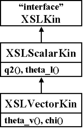
Figure 2: XSLKin class diagram. The arrows mean an inheritance.

The XSLKin user’s interface is used to declare all the kinematic variables needed by users of this tool. The variables are defined and computed at the second and third levels. The second level class, named XSLScalarKin, is used to compute the kinematic variables ($q^{2}$ and $\theta_{\ell}$) characterizing a B to pseudo-scalar meson decay. The third level class, named XSLVectorKin, is used to compute the two additional kinematic variables ($\theta_{V}$ and $\chi$) needed to describe fully a B to vector meson decay. The XSLVectorKin class already contains the values of $q^{2}$ and $\theta_{\ell}$ inherited from the XSLScalarKin class.

This tool was created with an interface structure to allow the eventual addition of a second set of classes to compute the kinematic variables differently. It is not clear at present if this second set of classes will ever be used.

3.2.2 The XSLEvtFFWeight tool

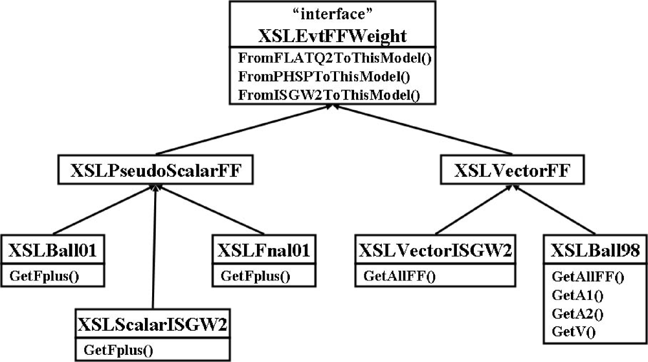
Figure 3: XSLEvtFFWeight class diagram. The arrows mean an inheritance.

The XSLEvtFFWeight tool architecture is shown in Fig. 3. The top level user’s interface of this tool is used to declare the functions needed by the tool’s user for reweighting an event. The second level of the diagram contains the classes that inherit from the XSLEvtFFWeight interface. In these classes, the functions declared in the interface are written out explicitly for the cases to be investigated i.e. for the B to pseudo-scalar meson decays in the XSLPseudoScalarFF class and for the B to vector meson decays in the XSLVectorFF class. These functions are used only to calculate the weight required to reweight the probability of generating an event from a given generator to a given form factor model. The form factors themselves as well as the kinematic parameters are computed in other classes. At the second level, the form factors are declared as pure virtual functions (GetFplus() and GetAllFF()) to be defined and computed at the third level. The third level classes are then used to compute these GetFplus() or GetAllFF() virtual functions of the second level i.e. the $f^{+}(q^{2})$ or $A_{1}(q^{2})$, $A_{2}(q^{2})$ and $V(q^{2})$ form factor values as a function of $q^{2}$ for various models.

3.3 How to implement new form factor models

The XSLEvtFFWeight tool has been created with a three-level structure to make it efficient in computing the reweighting among various form factor models: the form factors are modified at the third level while the other two levels remain the same independently of the form factors used. The third level class inherits from either the XSLPseudoScalarFF or XSLVectorFF class. The mathematical functions required to compute the form factor(s) as a function of $q^{2}$ are inserted in this class.

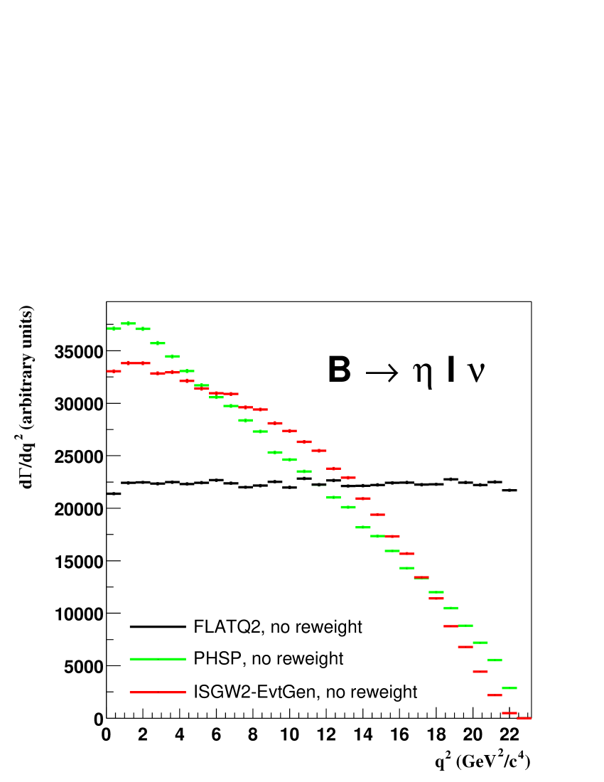
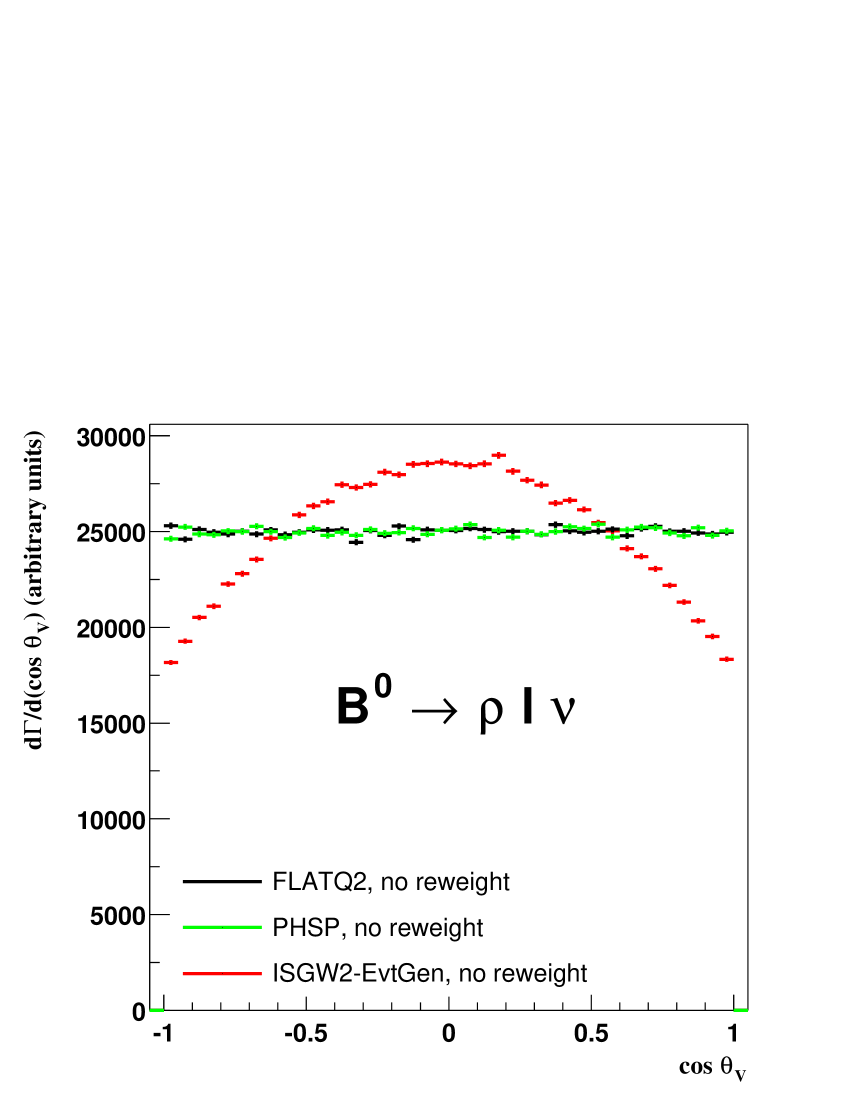
Figure 4: Events generated with the FLATQ2 (black), PHSP (pale grey) and ISGW2 (dark grey) generators: $q^{2}$ distributions for unweighted $B\rightarrow\eta\ell\nu$ decays (left panel); $\cos\theta_{V}$ distributions for unweighted $B^{0}\rightarrow\rho\ell\nu$ decays (right panel)

4 Validation of the reweighting technique and its software tool

In most simulations, the fully simulated events take into account the lepton’s Final State Radiation (FSR). However, the effect of FSR is not included in the reweighting formulas presented in Sect. 2.5. As a consequence, the XSLEvtFFWeight tool could yield the wrong weights unless corrected for FSR. We have found that the easiest way around this problem is to use the LorentzVector of the lepton calculated from the vectors of the other particles of the decay as those are not affected by FSR. This solution turns out to be very effective even in cases where the FSR modifies the lepton’s energy by several GeVs. As long as the same lepton is used to compute the kinematic angles and the event weight, the effect of the FSR on the form factor reweighting is negligible.

The histograms shown in this section were calculated with such lepton LorentzVectors. They are extracted from 1 million entries generated with no detector simulation. This generator information is what is used with full Monte Carlo simulation in real physics analyses. Only a small sample is presented in this section. More can be found in Ref. cote .

Our reweighting software has not been tested on any $B\rightarrow X_{c}\ell\nu$ decay but there is no reason to believe that the results will be any different from those obtained with the $B\rightarrow X_{u}\ell\nu$ decays.

4.1 Properties of the generators FLATQ2, PHSP and ISGW2

The properties of the three generators used in this work, and calculated with the XSLKin tool, are illustrated by the distributions displayed in Fig. 4. The distributions for all the decay modes of interest have been investigated cote and found to be as expected. Fig. 4 (left panel) shows that, both, the PHSP and ISGW2 generators yield low statistics at high $q^{2}$. This makes precise efficiency corrections difficult in this important region (particularly important for lattice QCD tests). Fig. 4 (right panel) shows that the PHSP and FLATQ2 $\cos\theta_{V}$ distributions are identical. This is also true for the $\cos\theta_{\ell}$ and $\chi$ angle distributions cote . Note that since the FLATQ2 generator yields flat distributions for all the variables ($\theta_{\ell},\theta_{V},\chi,q^{2}$) of interest, it allows a smooth reweighting over the full phase space. It is thus ideally suited to evaluate and correct the efficiencies as a function of these variables. To determine the analysis cuts required in realistic physics simulation, the FLATQ2 and PHSP generated events have to be reweighted.

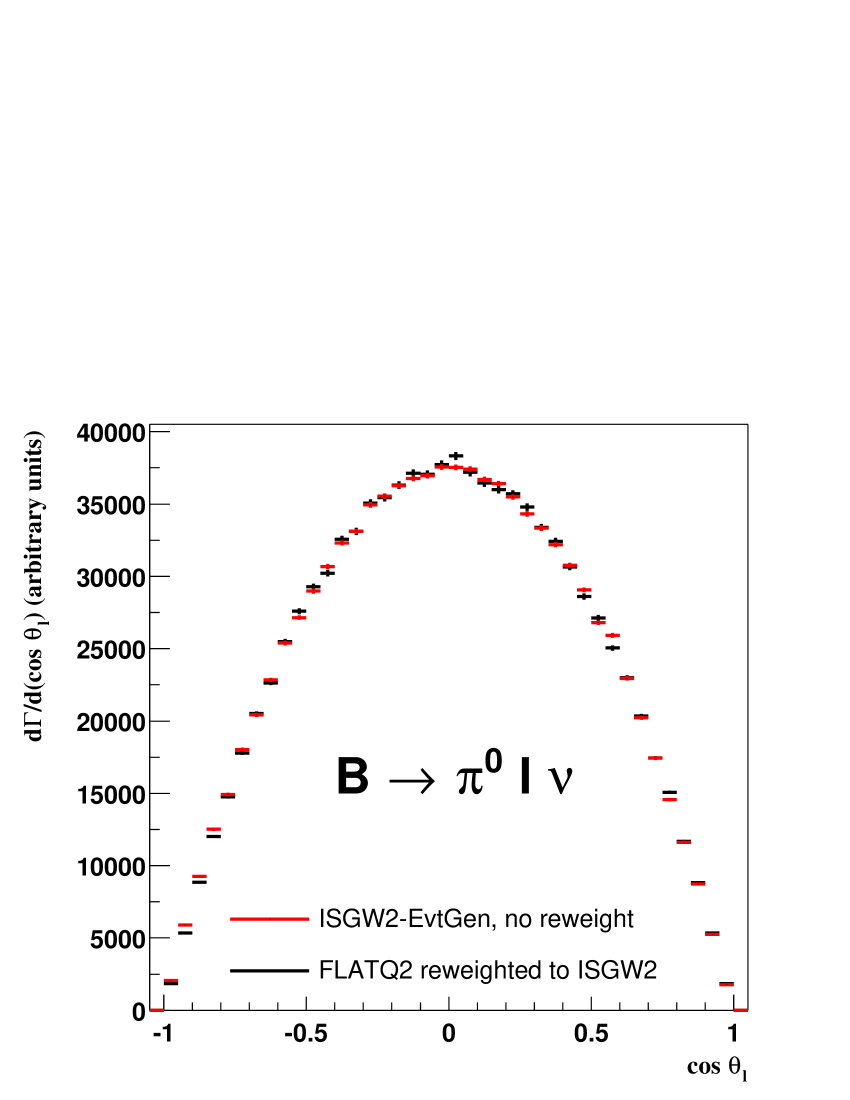
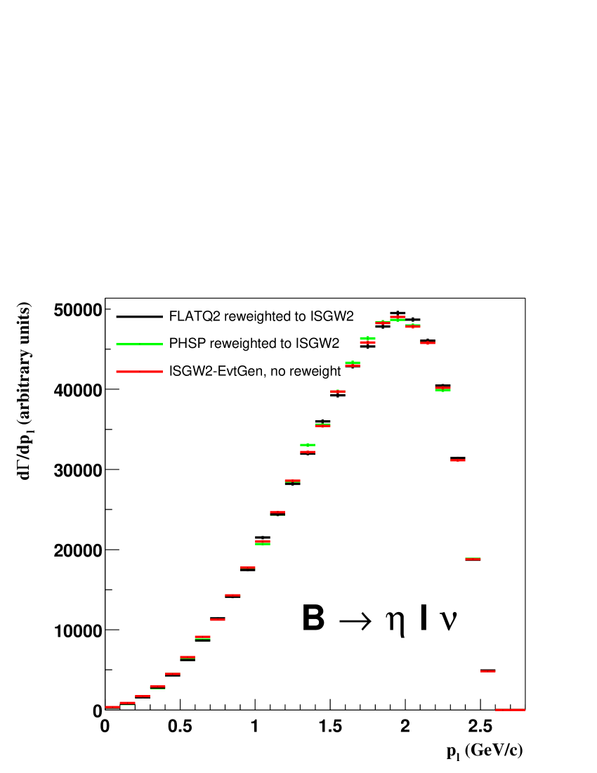
Figure 5: Pseudo-scalar decays. Events generated with a FLATQ2 generator and reweighted to the ISGW2 form factor hypothesis (black), events generated with a PHSP generator and reweighted to the ISGW2 form factor hypothesis (pale grey) and unweighted events generated directly with a ISGW2 generator (dark grey): comparison of $q^{2}$ distributions for $B\rightarrow\pi^{+}\ell\nu$ decay (left panel); comparison of $\cos\theta_{\ell}$ distributions for $B\rightarrow\pi^{0}\ell\nu$ decays (center panel); comparison of $p_{\ell}$ distributions, in the true B frame, for $B\rightarrow\eta\ell\nu$ decays (right panel).

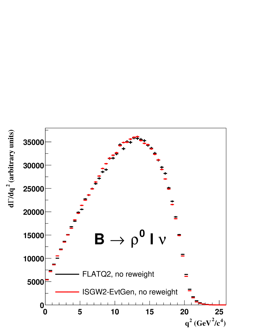
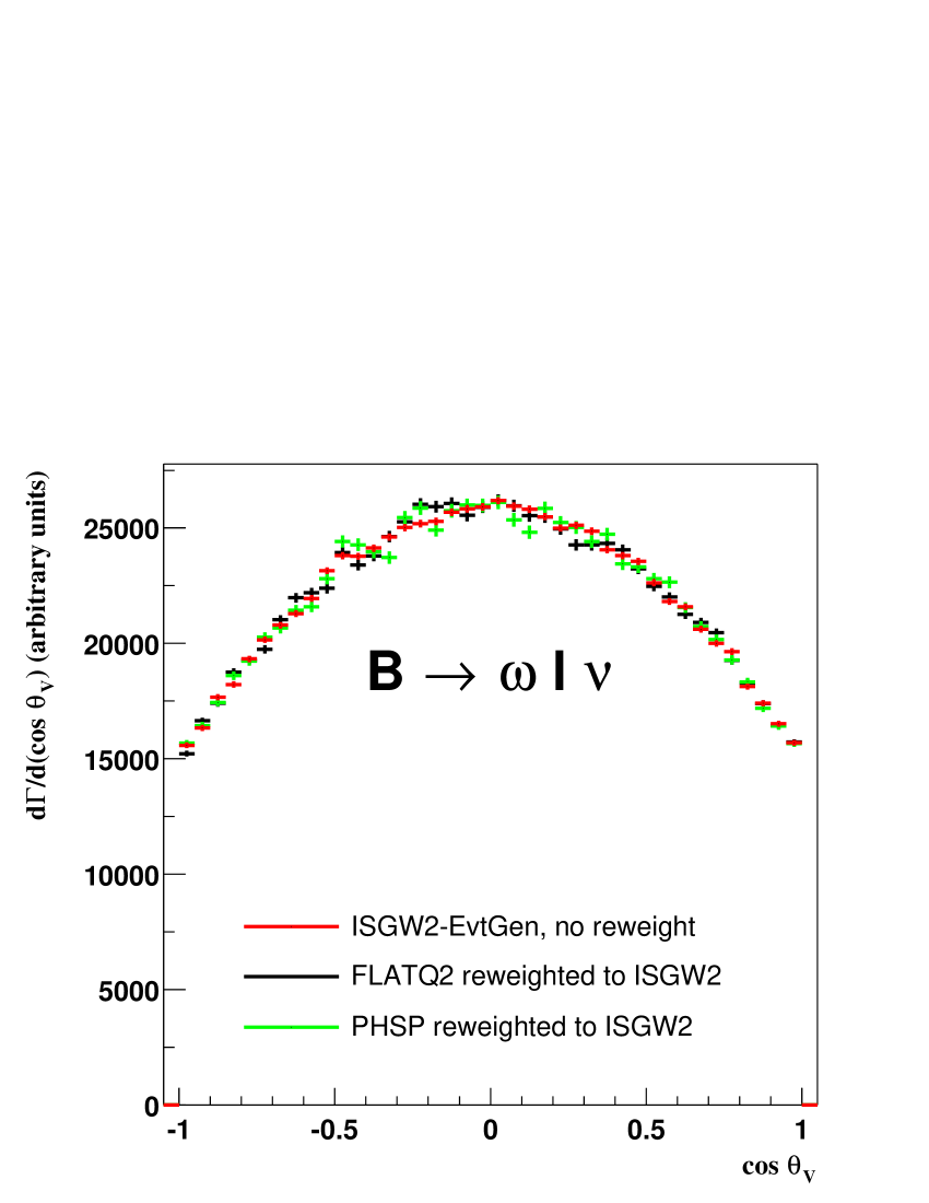
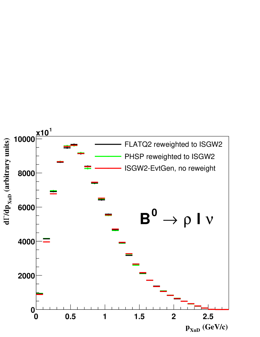
Figure 6: Vector meson decays. Events generated with a FLATQ2 generator and reweighted to the ISGW2 form factor hypothesis (black), events generated with a PHSP generator and reweighted to the ISGW2 form factor hypothesis (pale grey) and unweighted events generated directly with a ISGW2 generator (dark grey): comparison of $q^{2}$ distributions for $B\rightarrow\rho^{0}\ell\nu$ decays (left panel); comparison of $\cos\theta_{V}$ distributions for $B\rightarrow\omega\ell\nu$ decays (center panel); comparison of $p_{XuD}$ distributions, in the true B frame, for $B\rightarrow\rho^{+}\ell\nu$ decays (right panel). $p_{XuD}$ is the momentum of any daughter of the $X_{u}$ meson.

4.2 Reweighting of B to pseudo-scalar meson decays

Note that because of the three-level hierarchy of the XSLEvtFFWeight tool, it is sufficient to fully validate the software with only one generator. For this purpose, the ISGW2 generator was used. In this way, the XSLKin tool (Sect. 3.2.1) and the classes XSLEvtFFWeight, XSLPseudoScalarFF, XSLVectorFF, XSLScalarISGW2 and XSLVectorISGW2 (Sect. 3.2.2) are all validated. In the implementation of any new form factor model, it is then sufficient to ensure the correctness of the new form factor equations at the third level of the XSLEvtFFWeight tool (see Sect. 3.3).

As can be seen in Fig. 5, there is an excellent match between the distributions generated directly with the ISGW2 generator and those generated with the FLATQ2 or PHSP generators, and then reweighted to the ISGW2 form factor hypothesis with our software.

4.3 Reweighting of B to vector meson decays

Like for the reweighted pseudo-scalar meson decay results, there is the same excellent match (Fig. 6) when reweighting is applied to the distributions generated with the FLATQ2 or PHSP generators for vector meson decays.

4.4 Validity of the massless lepton approximation

Comparing various distributions generated with a standard ISGW2 generator to those generated with our form factor reweighting software allows us to test the validity of the massless approximation used in our reweighting software. This is the case since the standard code uses the exact formulas to compute the differential decay rates. Since the comparisons, done separately for electrons and muons, show the same good match, it can be concluded that the massless approximation is indeed justified for both, electrons and muons. An exemple of the quality of the match is displayed in Fig. 7.

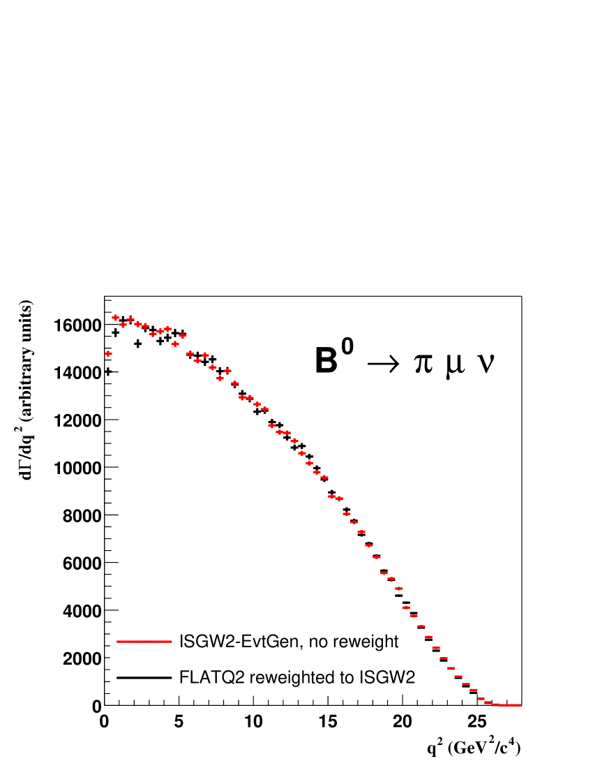
Figure 7: Comparison of $q^{2}$ distributions for $B\rightarrow\pi\mu\nu$ decays only. Events generated with a FLATQ2 generator and reweighted to the ISGW2 form factor hypothesis are shown in black while the unweighted events generated directly with a ISGW2 generator are shown in dark grey.

5 Improvements in measurements of $|V_{ub}|$

With our reweighting software, it is now easy to investigate the predictions of various form factor models, and to evaluate their impact on the experimental study of $B\rightarrow X_{u}\ell\nu$ decays. So far, two form factor models for pseudo-scalar and vector meson decays have been fully implemented in our software: the ISGW2 isgw2 model (used in the validation of the reweighting technique and its software tool) and a LCSR model from P. Ball et al. ball98 ball01 . Typical distributions for $q^{2}$ , $\cos\theta_{V}$ and $p_{\ell}$ (Fig. 5) deduced from these two models display a large difference while the $\cos\theta_{\ell}$ distributions for pseudo-scalar meson decays (Fig. 9, left panel) are not model-dependent, but those for vector meson decays (Fig. 9, right panel) are. This significant model-dependence shows why the values of the branching fraction and of the CKM matrix element $|V_{ub}|$, extracted from the study of exclusive semileptonic B meson decays, have such large theoretical errors.

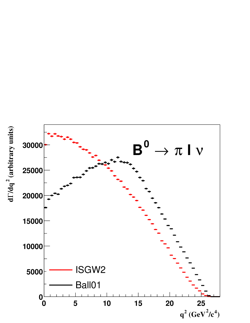
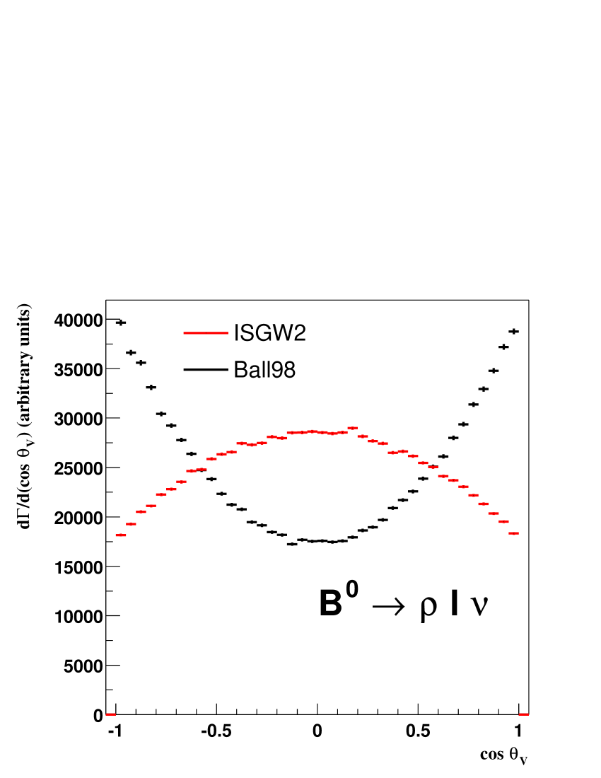
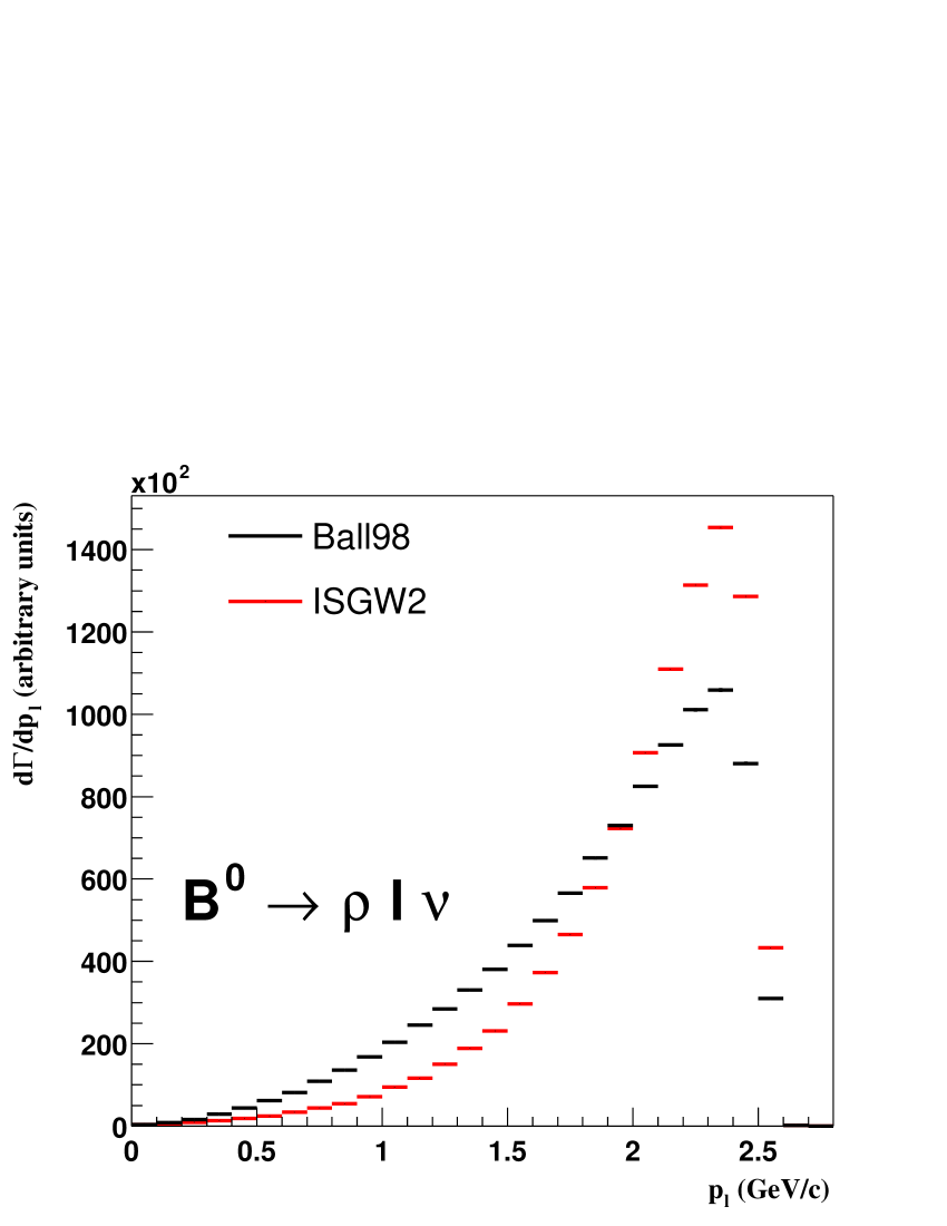
Figure 8: Events reweighted with the Ball01-LCSR form factor hypothesis (black), unweighted events generated directly with the ISGW2 form factor hypothesis (dark grey): comparison of $q^{2}$ distributions for $B\rightarrow\pi^{+}\ell\nu$ decays (left panel); comparison of $\cos\theta_{V}$ distributions for $B\rightarrow\rho^{+}\ell\nu$ decays (center panel); comparison of $p_{\ell}$ distributions for $B\rightarrow\rho^{+}\ell\nu$ decays (right panel).

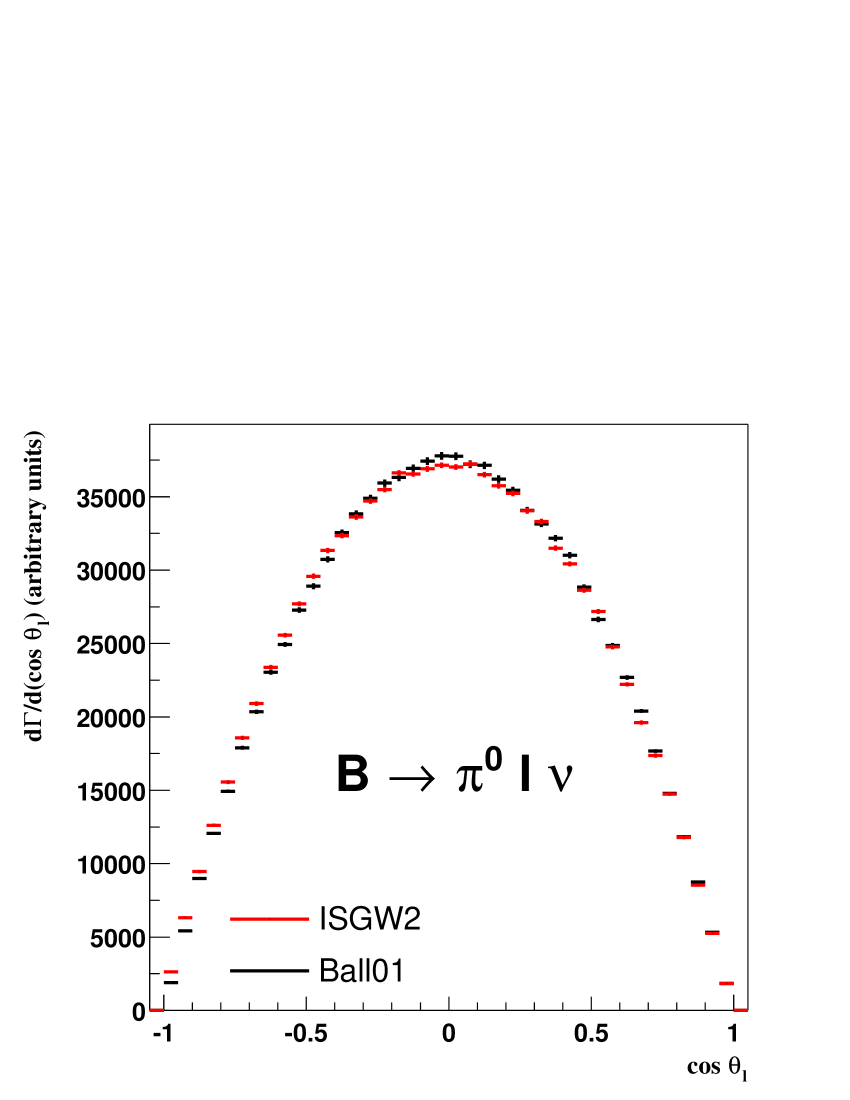
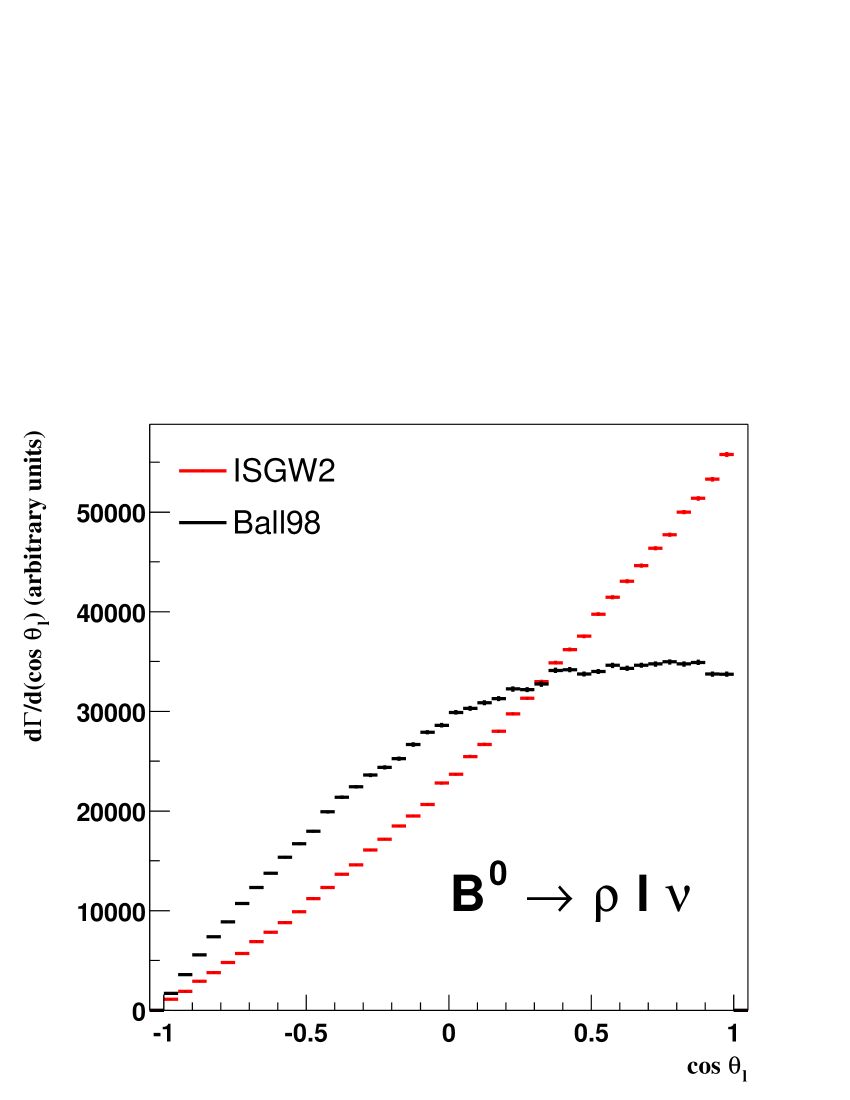
Figure 9: Events reweighted with the Ball01-LCSR form factor hypothesis (black), unweighted events generated directly with the ISGW2 form factor hypothesis (dark grey): comparison of $\cos\theta_{\ell}$ distributions for $B\rightarrow\pi^{0}\ell\nu$ pseudo-scalar meson decays (left panel); comparison of $\cos\theta_{\ell}$ distributions for $B\rightarrow\rho^{+}\ell\nu$ vector meson decays (right panel).

The most precise value to date of $|V_{ub}|$ obtained from the analysis of exclusive semileptonic B decays is the one given in Ref. pdg :

$$|V_{ub}|=(3.27\pm 0.13\pm 0.19^{+0.51}_{-0.45})\times 10^{-3}$$

where the first error is statistical, the second systematic and the third theoretical. It is clear that the theoretical error, of the order of 15%, due to form factor uncertainties, is by far the largest error. With our reweighting software tool, using our FLATQ2 generator, specially useful to determine the critical efficiencies of our experimental cuts as a function of $q^{2}$, we aim to reduce the theoretical error to approximately 5%. The integrated luminosity required to achieve this goal depends on the technique used to reconstruct the exclusive decay channel. With the neutrino reconstruction technique babar1 , and the more than 250 $fb^{-1}$, collected at the $\Upsilon(4S)$ resonance in both BaBar and Belle, and of the order of 500 $fb^{-1}$ expected within the next two years, a smaller theoretical error should be possible in the near future. With the recoil techniques babar2 , and for the other exclusive $\rho\ell\nu$, $\omega\ell\nu$, $\eta\ell\nu$ and $\eta^{\prime}\ell\nu$ decay channels, a few additional hundreds of $fb^{-1}$ will be required to extract a similar theoretical precision on $|V_{ub}|$.

With the soon to be available data from both BaBar and Belle, and with the neutrino reconstruction technique, a statistical error below 1% is possible. To achieve a theoretical error at a few percent level will require tight constraints on the form factors as a function of $q^{2}$. This can be accomplished by two methods.

In the first method, the measured differential decay distributions are compared to the corresponding ones predicted by various form factor models, as shown e.g. in Fig. 8. Our reweighting software tool will play a crucial role in these comparisons since it will allow a quick and easy test of all models without having to regenerate a complete MC production for each model. In this method, the efficiencies of the analysis cuts are computed with the model used to generate the distributions. With very high statistics, the method should allow us to keep a single form factor model as being the one closest to reality, thereby reducing the theoretical error on $|V_{ub}|$.

In the second method, the form factors will be measured directly with minimal model dependence. For example, for pseudo-scalar decays, the measured distributions will be fitted to Eq. 10 where the form factor is given e.g. ball04 by:

$$f^{+}(q^{2})=\frac{r_{1}}{1-q^{2}/m^{2}}+\frac{r_{2}}{\left(1-q^{2}/m^{2}\right)^{2}}$$

where $r_{1}$, $r_{2}$ and $m$ are the parameters to be fitted. Other functions will have to be investigated to obtain the systematic error engendered by the use of such functions. The small model dependence comes from the differential efficiencies, $\epsilon(q^{2}(,\theta_{\ell},\theta_{V},\chi))$, of the analysis cuts used to generate the measured distributions. To evaluate these efficiencies, the four kinematical variable distributions have to be binned, and the efficiencies are then determined for each bin.

In the limit of infinitesimal bins, the efficiency $\epsilon$ is independent of any model, as shown in Ref. [1]. But, of course, in any practical analysis, with finite statistics and limited kinematical variable resolutions, the bin size will be finite. This introduces a small model dependency which must be taken into account. It can be limited by the appropriate choice of analysis cuts since it can be shown cote that if the cuts are not correlated with the kinematic variables, then the efficiency is model-independent. The choice is greatly facilitated by the use of the FLATQ2 generator to determine the values of $\epsilon$, especially at very high values of $q^{2}$. It is also facilitated by the use of the form factor reweighting tool to select the experimental cuts to limit the correlation and thus the model dependence. The generator, combined with the software tool, will also yield a precise value of the small residual uncertainty due to the finite size of the bins. Once the parameters of the form factors are determined, they can be directly compared to any model predictions, thereby reducing the number of models and thus the theoretical uncertainty on $|V_{ub}|$.

6 Conclusions

A form factor reweighting technique and its software tool have been presented in this paper. Both have been validated with the ISGW2 form factor model as illustrated by the excellent match between the distributions generated with the FLATQ2 or PHSP generator, reweighted to the ISGW2 form factor hypothesis, and those generated directly with a ISGW2 generator. The object-oriented design of the software tool allows an easy and reliable implementation of any new form factor model, while optimizing the required CPU resources. The large differences, easily observed with our tool, in the distributions predicted by the ISGW2 and LCSR models for exclusive $B\rightarrow X_{u}\ell\nu$ decays show that a study of these decays will be very valuable in extracting the values of the form factors. Our work leads us to expect that both, our novel FLATQ2 generator and form factor reweighting tool, will play a key role in the next generation of exclusive $|V_{ub}|$ measurements, with largely reduced errors.

Acknowledgements We are grateful to M. S. Gill for providing Fig. 1. We wish to thank SLAC for its kind hospitality. This work was financially supported by NSERC (Canada).

References

- (1) D. Côté, BaBar Analysis Document 809, 2004 (unpublished)
- (2) D. Scora, N. Isgur, Phys. Rev. D 52, 2783 (1995)
- (3) A.X. El-Khadra, A.S. Kronfeld, P.B. Mackenzie, S.M. Ryan, J.N. Simone, Phys. Rev. D 64, 014502 (2001)
- (4) P. Ball, V.M. Braun, Phys. Rev. D 55, 5561 (1997)
- (5) P. Ball, R. Zwicky, JHEP 019, 0110 (2001)
- (6) J.D. Richman, P.R. Burchat, Rev. Mod. Phys. 67, 893 (1995)
- (7) L.K. Gibbons, Ann. Rev. Nucl. Part. Sci. 48, 121 (1998)
- (8) M. Battaglia, L. Gibbons in Phys. Lett. B 592, 1 (2004)
- (9) BaBar collaboration, B. Aubert et al., Phys. Rev. Lett. 90, 181801 (2003)
- (10) D. del Re (private communication)
- (11) P. Ball, R. Zwicky, arXiv:hep-ph/0406232 v1, June 2004