Determination of $\psi(2S)$ Total Number by Inclusive Hadronic Decay

Abstract    On the basis of the study of inclusive hadronic events, two methods are adopted to determine the number of produced $\psi(2S)$ events collected by BES in 2001$-$2002 run, which is $14.0\times 10^{6}$ with the uncertainty of 4%.

Key words    inclusive hadron, total number of $\psi(2S)$, uncertainty

1 Introduction

The BEijing Spectrometer (BES) is a general purpose solenoidal detector${}^{\mbox{\small\cite[cite]{[\@@bibref{}{detector}{}{}]}}}$ running at Beijing Electron Positron Collider (BEPC). The beam energy of BEPC is in the range from 1.5 GeV to 2.8 GeV with a design luminosity of $1.7\times 10^{31}\mbox{cm}^{-2}\mbox{s}^{-1}$ at 5.6 GeV center of mass energy. The main physics goal is to study the charm and $\tau$ physics. During 2001-2002 years’ running, about 14 million $\psi(2S)$ online hadronic events have been collected. On the basis of this large data sample, many physics analyses could be performed with an unprecedented precision.

The determination of the offline total number of $\psi(2S)$ event, $N^{TOT}_{\psi(2S)}$, is a foundational work in physics analysis, and in turn is the foundation of the further analysis study. In $\psi(2S)$ physics analysis, the calculation of the absolute branching ratio depends on $N^{TOT}_{\psi(2S)}$, whose error will be directly accounted into the error of the branching ratio of any being studied channel. Therefore, it is essential to work out the $N^{TOT}_{\psi(2S)}$ accurately and reliably. In principle, any decay channel with known branching ratio could be used to evaluate the total number of $\psi(2S)$:

$$N^{TOT}_{\psi(2S)}=\frac{N^{obs}_{f}}{\epsilon_{f}\cdot{\cal B}_{f}}~{},$$

where $N^{obs}_{f}$ is observed number of final state $f$ for a certain decay channel, $\epsilon_{f}$ and ${\cal B}_{f}$ are the corresponding efficiency and the branching ratio. It is obvious that the larger the branching ratio and the smaller the corresponding error, the more reliable the total number is. On such an extent, the inclusive hadron final state is a favorable process for the total number determination. The only disadvantage here lies in the difficulty to eliminate all kinds of backgrounds throughly. Therefore the meticulous studies have been made for the hadron event selection.

In the following sections, the hadron event selection is discussed firstly, then two methods are utilized to determine the total number of $\psi(2S)$ and the uncertainties from various sources are studied. At last, the final result is given.

For clearness and convenience, some notations which are to be used afterwards, are listed in the Table 1.

Table 1: Notations

Symbol	Meaning	Superscript	Meaning	Subscript	Meaning
$N$	Observed Number	$T$	Total	$h$	hadron final state
$m$	Selected Number	$P$	Peak region	$e$	$e^{+}e^{-}$ final state
$n$	“Pure” Hadron Number	$R$	Resonance
$\epsilon$	Efficiency	$C$	Continuum
$\sigma$	Cross section
$L$	Integrated Luminosity

In addition, there are two elementary relations among the five quantities $N$, $n$, $\epsilon$, $\sigma$, and $L$, that is

$${\displaystyle L=\frac{N}{\sigma}} N=L\cdot\sigma~{}~{},$$ or (1)

$${\displaystyle N=\frac{n}{\epsilon}} n=N\cdot\epsilon~{}~{}.$$ or (2)

The symbol with a tilde on it ($e.g.$ $\tilde{n}$, $\tilde{N}$, $etc.$), denotes the events obtained at the continuum region ($E_{beam}=3.665$ GeV), while others denote the events obtained at the resonance region ($E_{beam}=3.686$ GeV).

There are also two frequently used equalities, the first one for variables of the same process at different energy points:

$$\frac{\tilde{N}/\tilde{\sigma}}{N/\sigma}=\frac{\tilde{L}}{L}=\frac{\tilde{n}/(\tilde{\epsilon}\cdot\tilde{\sigma})}{n/(\epsilon\cdot\sigma)}~{}~{},\mbox{\hskip 5.69046ptor \hskip 5.69046pt}\frac{\tilde{n}}{n}=\frac{\tilde{L}\cdot\tilde{\sigma}}{L\cdot\sigma}\mbox{ ( for $\tilde{\epsilon}=\epsilon$ )}~{}~{};$$ (3)

the second one for variables of different process at the same energy points:

$$\frac{n^{I}/\epsilon^{I}}{n^{J}/\epsilon^{J}}=\frac{N^{I}}{N^{J}}=\frac{L\cdot\sigma^{I}}{L\cdot\sigma^{J}}=\frac{\sigma^{I}}{\sigma^{J}}~{}~{},\mbox{\hskip 5.69046ptor \hskip 5.69046pt}\frac{n^{I}}{n^{J}}=\frac{\epsilon^{I}\cdot\sigma^{I}}{\epsilon^{J}\cdot\sigma^{J}}~{}~{}.$$ (4)

2 Hadron Event Selection

For the hadron event selection, the detail information could be found in Refs. [2] and [3]. There is no particular event topology to require; instead cuts are made to reject major backgrounds: cosmic rays, beam associated backgrounds, two-photon process ($\gamma^{\ast}\gamma^{\ast}$), mis-identified “hadron” event from QED processes of $e^{+}e^{-}\rightarrow l^{+}l^{-},l=e,\mu,\tau$, and $e^{+}e^{-}\rightarrow\gamma\gamma$ followed by $\gamma$ conversion, and so forth. Most of these kinds of event have salient topology and could be eliminated by proper criteria. Events with at least two well reconstructed charged tracks within $|\cos\theta|\leq 0.8$ are selected (that is $N_{good}\geq 2$). The total energy deposited by an event in the BSC ($E_{sum}$) is required to be larger than 0.36 $E_{beam}$, in order to suppress the contamination from two-photon processes and beam associated backgrounds. Events with all tracks pointing to the same hemisphere in at least one of axial directions ($x$ or $y$ or $z$ direction) are removed to suppress beam associated backgrounds. (This requirement could be expressed quantitatively as $I_{ssi}\geq 1$, where $I_{ssi}$ is called the squared spatial distribution index.) For two-prong events, two additional cuts are applied to eliminate possible lepton pair backgrounds. The number of photons must be greater than one (that is $N_{real~{}\gamma}\geq 2$), and the acollinearity between two charged tracks, $\alpha_{Acol}$, must be greater than 10 degrees.

After the event selection, the fitting of double Gaussian plus a polynomial is applied to eliminate the remained background from beam associated backgrounds, see Fig. 2 and 2.

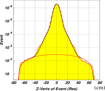
Figure 1: Vertex-Fit distribution ($E_{cm}=3.686$ GeV).

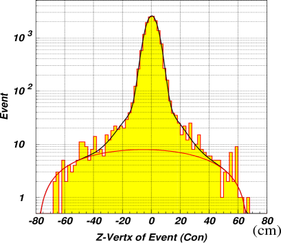
Figure 2: Vertex-Fit distribution ($E_{cm}=3.665$ GeV).

The global error analysis approach is adopted to obtain the uncertainties of selection cuts [3], as listed in Table 2:

Table 2: Error of hadron event selection.

Requirement	Error
$N_{good}\geq 2$	2.765 %
$E_{sum}>0.36E_{beam}$	2.544%
$I_{ssi}<1$	0.173 %
$N_{real\gamma}\geq 2$ (for $N_{good}=2$ )	0.042 %
$\alpha_{Acol}\geq 10^{\circ}$ (for $N_{good}=2$ )	0.157 %
Sum	3.765 %

In fact, there are many processes that could lead to hadron final state at $\psi(2S)$ resonance region, they could be divided into seven categories:

$$e^{+}e^{-} \rightarrow hadron\mbox{~{}~{}~{}(CH)}~{}~{},$$ (5)

$$e^{+}e^{-} \rightarrow \psi(2S)\rightarrow hadron\mbox{~{}~{}~{}(RH)}~{}~{},$$ (6)

$$e^{+}e^{-} \rightarrow J/\psi\rightarrow hadron\mbox{~{}~{}~{}($J/\psi$-H)}~{}~{},$$ (7)

$$e^{+}e^{-} \rightarrow \tau^{+}\tau^{-}\rightarrow hadron\mbox{~{}~{}~{}($\tau$-CH)}~{}~{},$$ (8)

$$e^{+}e^{-} \rightarrow \psi(2S)\rightarrow\tau^{+}\tau^{-}\rightarrow hadron\mbox{~{}~{}~{}($\tau$-RH)}~{}~{},$$ (9)

$$e^{+}e^{-} \rightarrow hadron^{\ast}\mbox{~{}~{}~{}(CH${}^{\ast}$)}~{}~{},$$ (10)

$$e^{+}e^{-} \rightarrow \psi(2S)\rightarrow hadron^{\ast}\mbox{~{}~{}~{}(RH${}^{\ast}$)}~{}~{},$$ (11)

where C represents the continuum process, R the resonance process, H hadron event, and H^∗ indicates the event which survives all aforementioned hadron selection cuts and is left in hadron sample from processes (10) and (11). Among above seven categories, only the hadron event from the first two processes are “pure” hadron event at $\psi(2S)$ peak region while others should be treated as backgrounds. Since hadron event from different process has almost the same event topology, the theoretical estimation method is used to evaluate the contamination of such kinds of backgrounds. According to the analysis in Ref. [3], two factors are introduced to subtract the hadronic background. If the pure hadron number is denoted as $n$ and the selected hadron number denoted as $m$, then it could be obtained

$$\gamma_{C}m^{C}_{had} = n^{C}_{had}~{}~{},$$ (12)

$$\gamma_{R}m^{R}_{had} = n^{R}_{had}~{}~{},$$ (13)

where

$$\gamma_{C} = 1-f_{J/\psi}-f_{C}=0.855~{}~{},$$

$$\gamma_{R} = 1-f_{R}=0.999~{}~{},$$

with

$$f_{J/\psi}=\frac{\sigma^{J/\psi}_{had}\cdot\epsilon^{J/\psi}_{had}}{\sigma^{C}_{had}\cdot\epsilon^{C}_{had}}~{}~{},$$

$$f_{C}=\sum\limits_{k=\tau,e,\mu,\gamma,\gamma^{*}}\frac{\sigma^{C}_{k}\cdot\epsilon^{C}_{k}}{\sigma^{C}_{had}\cdot\epsilon^{C}_{had}}~{}~{},$$

$$f_{R}=\sum\limits_{l=\tau,e,\mu,\gamma}\frac{B^{\psi(2S)}_{l}}{B^{\psi(2S)}_{h}}\cdot\frac{\epsilon^{R}_{l}}{\epsilon^{R}_{h}}~{}~{}.$$

Here all efficiencies are obtained from Monte Carlo simulation [3], and symbols $\tau,e,\mu,\gamma$ and $\gamma^{*}$ denote final states $\tau^{+}\tau^{-},e^{+}e^{-},\mu^{+}\mu^{-},\gamma\gamma$ and $\gamma^{*}\gamma^{*}$, respectively. For the continuum process, the production cross section $\sigma^{C}_{k}$ could be obtained from the corresponding Monte Carlo generator. For $\sigma^{C}_{had}$ and $\sigma^{J/\psi}_{had}$, they could be calculated by theoretical formulae with corresponding resonance parameters obtained from the scan experiment data [2, 4], which is about 15 nb and 1 nb, respectively. Since Monte Carlo generator does not give the cross section for resonance process, the ratio of branching fractions is used in the calculation of factor $f_{R}$ [3]. It should be pointed out that because the variation of $\sigma^{J/\psi}_{had}$ is fairly smooth at $\psi(2S)$ region, refer to Fig. 3, the contamination from $J/\psi$ decay is suitable to be treated as the continuum-like hadron background.

Figure 3: Cross section curve of $J/\psi$ resonance.

3 Determination of Total Number

3.1 Principle

The branching ratio of hadron final state, denoted as ${\cal B}_{h}$, can be acquired from PDG list [5] or from BES scan results [2]. If the number of selected hadron event from $\psi(2S)$ resonance is $n_{\psi(2S)\rightarrow had.}$, then

$$N^{TOT}_{\psi(2S)}=\frac{n_{\psi(2S)\rightarrow had.}}{\epsilon^{R}_{h}\cdot{\cal B}_{h}}~{}~{}.$$ (14)

However, the number of selected hadron event at a certain energy point is the combination of two parts (refer to Fig. 4), one from resonance process and the other from continuum one, that is

$$\begin{array}[]{ccccc}n_{had}&=&n_{\psi(2S)\rightarrow had.}&+&n_{e^{+}e^{-}\rightarrow had.}~{}~{},\\ \Downarrow&&\Downarrow&&\Downarrow\\ n^{T}_{h}&=&n^{R}_{h}(n^{P}_{h})&+&n^{C}_{h}~{}~{}.\end{array}$$ (15)

Therefore the key issue here is to distinguish the $n^{R}_{h}$ from the $n^{T}_{h}$. There are two methods, the fraction subtraction method and the normalization subtraction method, can be used to figure out the number of resonance event.

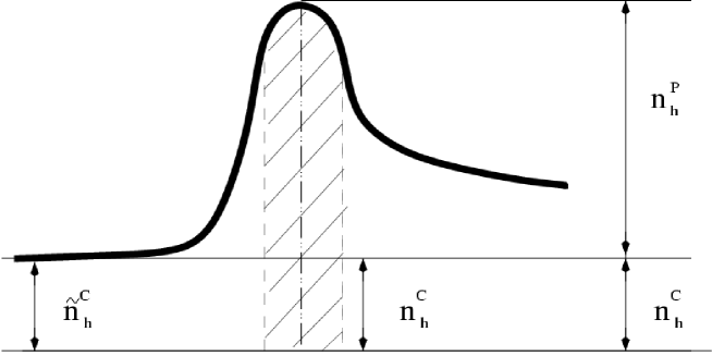
Figure 4: Fractional sketch of hadron number of different process. (The cross-hatched area in the figure indicates the data taking region.)

3.2 Fraction subtraction

Refer to Fig. 4, if the ratio of $n^{C}_{h}$ to $n^{P}_{h}$ could be estimated:

$$f=\frac{n^{C}_{h}}{n^{P}_{h}}~{}~{},$$

together with Eq. (15), the $n^{P}_{h}$ can be calculated as

$$n^{P}_{h}=\frac{n^{T}_{h}}{1+f}~{}~{}.$$ (16)

As to the factor $f$, from Eq. (4), it is easy to acquire

$$\frac{n^{C}_{h}}{n^{P}_{h}}=\frac{\epsilon^{C}_{h}\cdot\sigma^{C}_{h}}{\epsilon^{R}_{h}\cdot\sigma^{R}_{h}}~{}~{},\mbox{\hskip 5.69046ptor \hskip 5.69046pt}n^{C}_{h}=\frac{\epsilon^{C}_{h}\cdot\sigma^{C}_{h}}{\epsilon^{R}_{h}\cdot\sigma^{R}_{h}}\cdot n^{P}_{h}~{}~{},$$

so $f$ can be expressed as

$$f=\frac{\epsilon^{C}_{h}\cdot\sigma^{C}_{h}}{\epsilon^{R}_{h}\cdot\sigma^{R}_{h}}~{}~{}.$$ (17)

Combing Eqs. (14) and (16), it can be obtained

$$N^{TOT}_{\psi(2S)}=\frac{n^{T}_{h}}{{\cal B}_{h}\cdot\epsilon^{R}_{h}\cdot(1+f)}~{}~{}.$$ (18)

3.3 Normalization subtraction

The data taken far from the resonance region could be treated as the data of continuum, refer to Fig. 4, from Eq. (3), the number at continuum region $\tilde{n}^{C}_{h}$ could be transformed into that at resonance $n^{C}_{h}$ by a luminosity normalization factor

$$n^{C}_{h}=f_{T}\tilde{n}^{C}_{h}~{}~{},\hskip 56.9055ptf_{T}=\frac{\sigma^{C}_{h}\cdot L}{\tilde{\sigma}^{C}_{h}\cdot\tilde{L}}~{}~{},$$

where $f_{T}$ is the transformed factor. Combining with the relation $n^{T}_{h}=n^{P}_{h}+n^{C}_{h}$, the resonance number could be worked out

$$n^{P}_{h}=n^{T}_{h}-f_{T}\cdot\tilde{n}^{C}_{h}=n^{T}_{h}\cdot(1-f_{T}\cdot\frac{\tilde{n}^{C}_{h}}{n^{T}_{h}})~{}~{}.$$

In the expression of $f_{T}$, the luminosity $L$ is usually calculated by the continuum $e^{+}e^{-}$ event ($i.e.$ Bhabha event):

$$L=\frac{n^{C}_{e}}{\epsilon^{C}_{e}\cdot\sigma^{C}_{e}}~{}~{}~{}.$$

Similar to Eq. (16), at the continuum region, the number of events from the continuum process is expressed by the number of total selected events:

$$n^{C}_{e}=\frac{n^{T}_{e}}{1+f_{e}}~{}~{},\hskip 14.22636pt\tilde{n}^{C}_{e}=\frac{\tilde{n}^{T}_{e}}{1+\tilde{f}_{e}}~{}~{},\hskip 14.22636pt\tilde{n}^{C}_{h}=\frac{\tilde{n}^{T}_{h}}{1+\tilde{f}_{h}}~{}~{},$$

with

$$f_{e}={\displaystyle\frac{\epsilon^{R}_{e}\cdot\sigma^{R}_{e}}{\epsilon^{C}_{e}\cdot\sigma^{C}_{e}}}~{}~{},$$ (19)

$$\tilde{f}_{e}={\displaystyle\frac{\epsilon^{R}_{e}\cdot\tilde{\sigma}^{R}_{e}}{\epsilon^{C}_{e}\cdot\tilde{\sigma}^{C}_{e}}}~{}~{},$$ (20)

$$\tilde{f}_{h}={\displaystyle\frac{\epsilon^{R}_{h}\cdot\tilde{\sigma}^{R}_{h}}{\epsilon^{C}_{h}\cdot\tilde{\sigma}^{C}_{h}}}~{}~{}.$$ (21)

It should be noticed that the relation $\epsilon^{R,C}_{e,h}=\tilde{\epsilon}^{R,C}_{e,h}$ has been used in the above calculation.

Put all together, the total number can be calculated as

$$N^{TOT}_{\psi(2S)}=\frac{n^{T}_{h}}{{\cal B}_{h}\cdot\epsilon^{R}_{h}}\cdot\left(1-F_{T}\cdot M_{eh}\right)~{}~{},$$ (22)

where

$$F_{T}\equiv\frac{\sigma^{C}_{h}\cdot\tilde{\sigma}^{C}_{e}}{\tilde{\sigma}^{C}_{h}\cdot\sigma^{C}_{e}}\cdot\frac{(1+\tilde{f}_{e})}{(1+f_{e})}\cdot\frac{1}{(1+\tilde{f}_{h})}~{}~{},$$ (23)

$$M_{eh}=\frac{n^{T}_{e}}{\tilde{n}^{T}_{e}}\cdot\frac{\tilde{n}^{T}_{h}}{n^{T}_{h}}~{}~{},$$ (24)

with factors $f_{e}$, $\tilde{f}_{e}$, and $\tilde{f}_{h}$ are given in Eqs. (19), (20) and (21).

3.4 Correction

As mentioned in section 2, after the hadron event selection, the selected hadron number $m$ instead of pure one $n$ is obtained. The relation between $m$ and $n$ is given in Eq. (12) and  (13), that is

$$\gamma_{C}(m^{C}_{h},\tilde{m}^{C}_{h}) = (n^{C}_{h},\tilde{n}^{C}_{h})~{}~{},$$

$$\gamma_{R}(m^{R}_{h},\tilde{m}^{R}_{h}) = (n^{R}_{h},\tilde{n}^{R}_{h})~{}~{}.$$

Notice that

$$m^{T}_{h}=m^{P}_{h}+m^{C}_{h}~{}~{},~{}~{}~{}~{}~{}(m^{P}_{h}=m^{R}_{h})~{}~{},$$

then

$$m^{T}_{h}=\frac{n^{P}_{h}}{\gamma_{R}}+\frac{n^{C}_{h}}{\gamma_{C}}=\frac{n^{P}_{h}}{\gamma_{R}}+\frac{fn^{P}_{h}}{\gamma_{C}}=n^{P}_{h}\cdot\left(\frac{1}{\gamma_{R}}+\frac{f}{\gamma_{C}}\right)~{}~{},$$

that is

$$n^{P}_{h}=\frac{m^{T}_{h}}{\displaystyle\left(\frac{1}{\gamma_{R}}+\frac{f}{\gamma_{C}}\right)}~{}~{}.$$

So the formula for the fraction subtraction method now becomes

$$N^{TOT}_{\psi(2S)}=\frac{m^{T}_{h}}{{\cal B}_{h}\cdot\epsilon^{R}_{h}\cdot(1+f)\cdot\delta_{\gamma_{1}}}~{}~{},$$ (25)

where $\delta_{\gamma_{1}}$ is defined as

$$\delta_{\gamma_{1}}=\frac{\displaystyle\frac{1}{\gamma_{R}}+\frac{f}{\gamma_{C}}}{\displaystyle 1+f}~{}~{}.$$ (26)

For the normalization subtraction method, the corresponding corrected formula could be obtained similarly and the final result is

$$N^{TOT}_{\psi(2S)}=\frac{m^{T}_{h}}{\gamma_{R}\cdot{\cal B}_{h}\cdot\epsilon^{R}_{h}}\cdot\left(1-{\cal F}_{T}\cdot{\cal M}_{eh}\right)~{}~{},$$ (27)

where

$${\cal M}_{eh}=\frac{n^{T}_{e}}{\tilde{n}^{T}_{e}}\cdot\frac{\tilde{m}^{T}_{h}}{m^{T}_{h}}~{}~{},$$ (28)

and

$${\cal F}_{T}=F_{T}/\delta_{\gamma_{2}}~{}~{},~{}~{}~{}~{}~{}~{}\delta_{\gamma_{2}}\equiv\frac{\displaystyle 1+\frac{\gamma_{C}}{\gamma_{R}}\tilde{f}_{h}}{1+\tilde{f}_{h}}~{}~{},$$ (29)

here $F_{T}$ is just as that defined in Eq. (23).

3.5 Numerical Calculation

By the virtue of Eqs. (25) and (27), $N^{TOT}_{\psi(2S)}$ could be worked out. For convenience, all numbers relevant to total number calculation are summarized in Table 3.

Table 3: Event number, efficiency and cross section.

Final state		$hadron$		$e^{+}e^{-}$
Region		Resonance	Continuum	Resonance	Continuum
Event number		$m^{T}_{h}=10634586.0$	$\tilde{m}^{T}_{h}=13937.7$	$n^{T}_{e}=1190613$	$\tilde{n}^{T}_{e}=54415$
$m^{fit}_{h}$ ($\Delta m^{fit}_{h}$)		($\Delta m^{T}_{h}=11688.2$)	($\Delta\tilde{m}^{T}_{h}=817.2$)
Efficiency	Resonance	$\epsilon^{R}_{h}=0.753$	$\tilde{\epsilon}^{R}_{h}\approx\epsilon^{R}_{h}$	$\epsilon^{R}_{e}=0.761$	$\tilde{\epsilon}^{R}_{e}=\epsilon^{R}_{e}$
	process	($\Delta\epsilon^{R}_{h}=0.012$)
	Continuum	$\epsilon^{C}_{h}=0.716$	$\tilde{\epsilon}^{C}_{h}\approx\epsilon^{C}_{h}$	$\epsilon^{C}_{e}=0.708$	$\tilde{\epsilon}^{R}_{e}=\epsilon^{R}_{e}$
	process	($\Delta\epsilon^{R}_{h}=0.010$)
Cross	Resonance	$\sigma^{R}_{h}=676.277$	$\tilde{\sigma}^{R}_{h}=0.266$	$\sigma^{R}_{e}=4.053$	$\tilde{\sigma}^{R}_{e}=0.00158$
section	process
($nb$)	Continuum	$\sigma^{C}_{h}=15.495$	$\tilde{\sigma}^{C}_{h}=15.673$	$\sigma^{C}_{e}=80.423$	$\tilde{\sigma}^{C}_{e}=81.349$
	process
Trigger efficiency $\sharp$		Correction factor
$\epsilon^{trg}_{h}=0.99924$		$\gamma_{R}=0.999$		$\gamma_{C}=0.855$

$\sharp$: the trigger efficiency is obtained from Ref. [6] written by Dr. Fu ChengDong.

$N^{TOT}_{\psi(2S)}$ is worked out to be either 14.05$\times 10^{6}$ for Fraction method or 14.04$\times 10^{6}$ for Normalization method.

4 Error Analysis

4.1 Classification

Formally, by the virtue of Eqs. (18) and (22), the formula to calculate the total number can be written as

$$N^{TOT}_{\psi(2S)}=\frac{n^{T}_{h}}{{\cal B}_{h}\cdot\epsilon^{R}_{h}}\cdot G_{i}~{}~{}~{},$$ (30)

where $G_{i}$ is a correction factor defined as

$$G_{i}=\left\{\begin{array}[]{ll}G_{1}={\displaystyle\frac{1}{1+f}}~{}~{},&\mbox{for the fraction method;}\\ G_{2}=(1-F_{T}\cdot M_{eh})~{}~{},&\mbox{for the normalization method.}\end{array}\right.$$

The error of $N^{TOT}_{\psi(2S)}$ comes from the components of Eq. (30), such as $n^{T}_{h}$, $\epsilon^{R}_{h}$, ${\cal B}_{h}$, and $G_{i}$, the error of which will be discussed one by one.

4.2 Uncertainty of selected number $m^{T}_{h}$

For the selected number $m^{T}_{h}$, there are three sources of uncertainty:

1. Fitting uncertainty
   The uncertainty of fitted number could be obtained from the corresponding error of fitting parameters which are used to calculate the number (refer to Table 3), that is

   $$\nu_{fit}(m^{T}_{h})=\frac{\Delta m^{fit}_{h}}{m^{fit}_{h}}=0.11\%$$

2. Statistic uncertainty
   According to statistic principle,

   $$\nu_{sta}(m^{T}_{h})=\frac{1}{\sqrt{m^{T}_{h}}}=0.03\%$$

3. Selection uncertainty
   According to the study of section 1, the selection uncertainty reflects the inconsistency between data ($m^{T}_{h}$) and Monte Carlo ($\epsilon^{R}_{h}$), so the uncertainty of $\epsilon^{R}_{h}$ is also included in this term which is

   $$\nu_{sel}\left(\frac{m^{T}_{h}}{\epsilon^{R}_{h}}\right)=3.77\%~{}~{}.$$

4. Effect due to beam energy fluctuation
   As it is mentioned in footnote 3, the data are actually taken within an enegy range (refer to the sketch description in Fig. 4), so the ratio between $\sigma^{C}_{h}/\sigma^{R}_{h}$ will vary with the actual beam energy which may be different for different beam-injection. Usually, each beam-injection includes 3$-$5 runs. As an estimation, all runs are grouped with every 3, 4 or 5 runs, then the ratios of selected hadron number ($n^{T}_{h}$) to that of $e^{+}e^{-}$ number ($n^{T}_{e}$) are worked out, which denoted as $r_{he}(i)$ with $i$ indicating the grouped run number. Fig. 5 shows the $r_{he}$ distribution for different grouped-run number. The maximum value of $r_{he}(i)$ corresponds to the peak cross section. Taking the experimental statistic fluctuation into account, the value 10 is adopted as the position of the peak cross section. The uncertainty from the beam energy fluctuation effect is estimated as follows

   $$\nu_{exp}=\frac{n^{T}_{h}/(1+f)}{\sum\limits_{i}n^{T}_{h}(i)/[1+f(i)]}~{}~{},$$

   with

   $$f(i)=\frac{\epsilon^{C}_{h}\cdot\sigma^{C}_{h}}{\epsilon^{R}_{h}\cdot\sigma^{R}_{h}}\cdot\frac{10}{r_{he}(i)}~{}~{}.$$

   For different grouped-run cases, $\nu_{exp}$ is almost the same, which is 0.23 %.

   

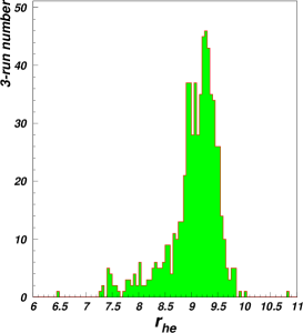
   (a) grouped with 3 runs

   

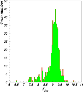
   (b) grouped with 4 runs

   

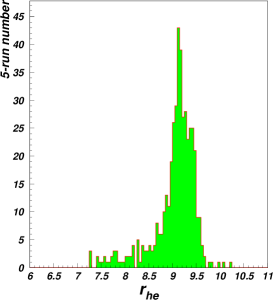
   (c) grouped with 5 runs

   Figure 5: $r_{he}$ distributions for different grouped-run number.

4.3 Uncertainty of branching ratio ${\cal B}_{h}$

There are two ${\cal B}_{h}$ values, one from PDG2002 and the other from $\psi(2S)$ scan experiment:

$$\begin{array}[]{rcl}{\cal B}_{h}(\mbox{PDG}2002)&=&(98.10\pm 0.30))\%~{}~{},\\ {\cal B}_{h}(\psi(2S)\mbox{ scan})&=&(97.79\pm 0.15)\%~{}~{}.\end{array}$$

In the total number calculation the ${\cal B}_{h}$ value form PDG2002 is used. However as a conservative estimation, the difference between above two values is used as the uncertainty of ${\cal B}_{h}$, that is

$$\nu({\cal B}_{h})=0.32\%~{}~{}.$$

4.4 Uncertainty of correction factor $G_{i}$

For $G_{1}$, the uncertainty due to different $f$ could be calculated as follows

$$\nu(G_{1})={\displaystyle\left|\frac{N^{TOT}_{\psi(2S)}(f)-N^{TOT}_{\psi(2S)}(f^{\prime})}{N^{TOT}_{\psi(2S)}(f)}\right|}=\left|\frac{\displaystyle\frac{1}{1+f}-\frac{1}{1+f^{\prime}}}{\displaystyle\frac{1}{1+f}}\right|=\left|\frac{\displaystyle f^{\prime}-f}{\displaystyle 1+f^{\prime}}\right|~{}~{}.$$

According to the definition of $f$, Eq. (17), the uncetainty of $f$ mainly comes from the statistics of $\epsilon^{C}_{h}$ and $\epsilon^{R}_{h}$, both of which are $1/\sqrt{50000}$. Notice $f=0.02179$ is a small quantity and the maximum difference between $f$ and $f^{\prime}$ is also small, so

$$\nu(G_{1})\approx|1-f|\cdot\Delta\approx 0.88\%~{}~{},$$

where $\Delta\equiv|f-f^{\prime}|_{max}=2/\sqrt{50000}$.

For $G_{2}$, the uncertainty due to different $G_{2}$ could be calculated as follows

$$\nu(G_{2})={\displaystyle\left|\frac{N^{TOT}_{\psi(2S)}(G_{2})-N^{TOT}_{\psi(2S)}(G_{2}^{\prime})}{N^{TOT}_{\psi(2S)}(G_{2})}\right|}=\left|\frac{F_{T}\cdot M_{eh}-F^{\prime}_{T}\cdot M^{\prime}_{eh}}{1-F_{T}\cdot M_{eh}}\right|~{}~{}.$$

Notice $F_{T}(=0.932)$ approximates to one, so the difference of total number calculated with $F_{T}=1$ and with $F_{T}\neq 1$, is treated as the error from factor $F_{T}$, that is

$$\nu(F_{T})={\displaystyle\left|\frac{M_{eh}\cdot(F_{T}-1)}{1-F_{T}\cdot M_{eh}}\right|}=0.20\%~{}~{}.$$

Notice $M_{eh}$ consists of two pairs of ratio, so the systematic error of numerator and denominator will cancel automatically, only the statistic error is left, which is

$$\Delta M_{eh}=\sqrt{\frac{1}{n^{T}_{e}}+\frac{1}{\tilde{n}^{T}_{e}}+\frac{1}{\tilde{n}^{T}_{h}}+\frac{1}{n^{T}_{h}}}=0.95\%~{}~{},$$

so the error due to different $M_{eh}$ could be calculated as

$$\nu(M_{eh})={\displaystyle\left|\frac{F_{T}\cdot(M_{eh}-M^{\prime}_{eh})}{1-F_{T}\cdot M_{eh}}\right|}\leq{\displaystyle\left|\frac{F_{T}\cdot\Delta M_{eh}}{1-F_{T}\cdot M_{eh}}\right|}\approx 0.91\%~{}~{}.$$

Then the uncertainty for $G_{2}$ is

$$\nu(G_{2})=\sqrt{\nu^{2}(F_{T})+\nu^{2}(M_{eh})}=0.94\%~{}~{}.$$

4.5 Other uncertainty

The other effects which could lead to the uncertainty include the correction factor $\gamma_{C}$, $\gamma_{R}$, trigger efficiency and so forth. All these uncertainties are regarded as less than 0.5%. In addition, Monte Carlo sample is used as input to test the bias of our method. The error from such bias is about 0.6%.

4.6 Summary

Put all things together, the synthetic uncertainties are summarized in Table 4.

Table 4: Error summary.

Source		Uncertainty
$n^{T}_{h}$	Fitting	0.11 %
	Statistic	0.03 %
($\&\epsilon^{R}_{h}$)	Selection	3.77 %
	$E_{beam}$ fluctuation	0.23 %
${\cal B}_{h}$		0.32 %
$G_{i}$	$G_{1}$	0.88 %
	$G_{2}$	0.94 %
Other		(0.5$\oplus$0.6) %
Total	Method 1	3.97 %
	Method 2	3.98 %

Note: Method 1 for Fraction method; Method 2 for Normalizaion method.

5 Result and Discussion

The final total number of $\psi(2S)$ event with corresponding error is

$$N^{TOT}_{\psi(2S)}=\left\{\begin{array}[]{ll}14.05\times(1\pm 3.97\%)\times 10^{6}~{}~{},\mbox{~{}~{}(Fraction Method)~{};}\\ 14.04\times(1\pm 3.98\%)\times 10^{6}~{}~{},\mbox{~{}~{}(Normalization Method)~{}.}\end{array}\right.$$

Notice Eqs. (18) and (22), two methods, the fraction method and the normalization method, correlated closely with each other and the difference between two methods for the central value is actually less than one per mille. Furthermore, the difference of the uncertainty for two methods is also fairly small. Therefore, the central value of the offline total number of $\psi(2S)$ event could be regarded as $14.0\times 10^{6}$, and the uncertainty could conservatively be estimated as 4%.

Thanks are due to Prof. J. C. Chen and Prof. D. H. Zhang for their help about Monte Carlo simulation.

References

• [1] BAI Jing-Zhi et al. Nucl. Instr. Meth., 1999,A344:319-334;
BAI Jing-Zhi et al. Nucl. Instr. Meth., 2001,A458:627-637
• [2] BAI Jing-Zhi et al. Phys. Lett., 2002, B550: 24-32
• [3] Mo Xiao-Hu, Study of Inclusive Hadronic Event, (2003.6), BES Memo
• [4] BAI Jing-Zhi et al. Phys. Lett., 1995, B355: 374-380.
• [5] Particle Data Group, Hagiwara K et al. , Phys. Rev. 2002, D66:010001
• [6] FU Cheng-Dong, Measurement of the Trigger Efficiency of $\psi^{\prime}$, (Feb. 27, 2003), BES Memo