Extraction of the $b$-quark shape function parameters using the Belle $B\rightarrow X_{s}\gamma$ photon energy spectrum

Abstract

We determine the $b$-quark shape function parameters, $\Lambda^{\mathrm{SF}}$ and $\lambda_{1}^{\mathrm{SF}}$ using the Belle $B\rightarrow X_{s}\gamma$ photon energy spectrum. We assume three models for the form of the shape function; Exponential, Gaussian and Roman.

I Introduction

The off-diagonal element $V_{ub}$ in the CKM matrix is extracted from measurements of the $B\rightarrow X_{u}\ell\nu$ process in the limited region of lepton momentum CLEOendpt , or the hadronic recoil mass $M_{X}$ BaBar , or $M_{X}$ and the leponic invariant mass squared $q^{2}$ Kakuno where the contribution of background from the $B\to X_{c}\ell\nu$ process is suppressed. In order to determine $|V_{ub}|$ we need to extrapolate measured rates from such limited regions to the whole phase space. This extrapolation factor is evaluated using a theoretical prediction that takes into account the residual motion of the $b$-quark inside the $B$ meson, so called “Fermi motion” FN . Fermi motion is included in the heavy quark expansion by resumming an infinite set of leading-twist corrections into a shape function of the $b$-quarkNeub ; Ural ; NeuMan . Since the shape function is not calculable theoretically, it has to be determined experimentally.

The best way is to make use of the photon energy spectrum for $B\rightarrow X_{s}\gamma$ since both the inclusive decay spectra in $B\rightarrow X_{u}\ell\nu$ and $B\rightarrow X_{s}\gamma$ are expressed by the same shape function up to leading order of $1/m_{b}$ in the heavy quark expansion KN ; Bigi . The first results were obtained by CLEO Gibbons , but the errors of the shape function parameters are rather large. Therefore the uncertainty of the shape function dominates the theoretical error of $|V_{ub}|$ at present. Belle has recently provided more precise data than CLEO of the $B\rightarrow X_{s}\gamma$ photon spectrum Koppenburg . We report on the results of determination of the shape function parameters using the Belle $B\rightarrow X_{s}\gamma$ data.

II Procedure

We used a method based on that devised by the CLEO collaborationAnderson . We fit Monte Carlo (MC) simulated spectra to the raw data photon energy spectrum. “Raw” refers to the spectra that are obtained after the application of the $B\rightarrow X_{s}\gamma$ analysis cuts. The use of “raw” spectra correctly accounts for the Lorentz boost from the $B$ rest frame to the center of mass system, energy resolution effects and avoids unfolding. The method is as follows;

1. Assume a shape function model.

2. Simulate the photon energy spectrum for a certain set of parameters; $(\Lambda^{\mathrm{SF}},\lambda_{1}^{\mathrm{SF}})$.

3. Perform a $\chi^{2}$ fit of the simulated spectrum to the data where only the normalization of the simulated spectrum is floated and keep the resultant $\chi^{2}$ value.

4. Repeat steps 2-3 for different sets of parameters to construct a two dimensional grid with each point having a $\chi^{2}$.

5. Find the minimum $\chi^{2}$ on the grid and all points on the grid that are one unit of $\chi^{2}$ above the minimum.

6. Repeat steps 1-5 for a different shape function model.

II.1 Shape function models

Three shape function forms suggested in the literature are employed; Exponential, Gaussian and RomanBigi ; KN . These are described in Table 1. The shape function $F$ is a function of $k_{+}(\equiv k_{0}-k_{3})$, where $k_{\mu}$ is the residual momentum of the $b$-quark in the $B$ meson, defined through

$$p_{b,\mu}=m_{b}v_{\mu}+k_{\mu},$$ (1)

where $v_{\mu}=(1,0,0,0)$ and $k_{3}$ is the $k$ component along the direction of the $u$-quark. The shape function is parameterized by $\Lambda^{\mathrm{SF}}$ and $\lambda_{1}^{\mathrm{SF}}$. These parameters are related to the $b$ quark mass, $m_{b}$, and the average momentum squared of the $b$ quark, $\mu_{\pi}^{2}$, via the relations,

$$\Lambda^{\mathrm{SF}}=M_{B}-m_{b}$$ (2)

and

$$\lambda_{1}^{\mathrm{SF}}=-\mu_{\pi}^{2},$$ (3)

where $M_{B}$ is the mass of the $B$ meson. Up to leading order in the non-perturbative dynamics the shape function is universal in describing the $b$-quark Fermi motion relevant to $b$-to-light quark transitions. The lepton and photon energy spectra in $B\rightarrow X_{u}l\nu$ and $B\rightarrow X_{s}\gamma$ decays are given by the convolution of the respective parton-level spectra with the shape function. Example shape function curves are plotted in Figure 1(a).

Shape Function	Form
Exponential	$F(k_{+};a)=N(1-x)^{a}e^{(1+a)x}$
Gaussian	$F(k_{+};c)=N(1-x)^{c}e^{-b(1-x)^{2}}$
	where $b=\left(\Gamma(\frac{c+2}{2})/\Gamma(\frac{c+1}{2})\right)^{2}$
Roman	$F(k_{+};\rho)=N\frac{\kappa}{\sqrt{\pi}}\exp\big{\{}-\frac{1}{4}\big{(}\frac{1}{\kappa}\frac{\rho}{1-x}-\kappa(1-x)\big{)}^{2}\big{\}}$
	where $\kappa=\frac{\rho}{\sqrt{\pi}}e^{\rho/2}K_{1}(\rho/2)$
where $x=k_{+}/\Lambda^{\mathrm{SF}}$
$-m_{b}\leq k_{+}\leq\Lambda^{\mathrm{SF}}$
and $a,c,\rho,N$ are chosen
to satisfy
$A_{0}=1$, $A_{1}=0$, $A_{2}=-\lambda_{1}^{\mathrm{SF}}/3$,
where $A_{n}=\int k_{+}^{n}F(k_{+})dk_{+}$

Table 1: The three models used for the shape function forms

Figure 1: Shape function model curves for Exponential $(\Lambda^{\mathrm{SF}},\lambda_{1}^{\mathrm{SF}})=(0.66,-0.40)$, Gaussian $(\Lambda^{\mathrm{SF}},\lambda_{1}^{\mathrm{SF}})=(0.63,-0.40)$, and Roman $(\Lambda^{\mathrm{SF}},\lambda_{1}^{\mathrm{SF}})=(0.66,-0.39)$, where $\Lambda^{\mathrm{SF}}$ and $\lambda_{1}^{\mathrm{SF}}$ are measured in units of $\mathrm{GeV}/c^{2}$ and $\mathrm{GeV}^{2}/c^{2}$ respectively.

II.2 Monte Carlo simulated photon energy spectrum

We generate $B\rightarrow X_{s}\gamma$ MC events according to the Kagan and Neubert prescription for each set of the shape function parameter values KN . The generated events are then simulated for the detector performance using the Belle detector simulation program. Afterwards $B\rightarrow X_{s}\gamma$ analysis cuts are applied to the MC events to obtain the raw photon energy spectrum in the $\Upsilon(4S)$ rest frame Koppenburg .

II.3 Fitting the spectrum

For a given set of shape function parameters, a $\chi^{2}$ fit of the MC simulated photon spectrum to the raw data spectrum is performed in the interval, $1.5<E^{*}_{\gamma}/\mathrm{GeV}<2.8$. The normalization parameter is floated in the fit. The raw spectrum is plotted in Figure 2, the errors include both statistical and systematic errors. The latter are dominated by the estimation of the $B\bar{B}$ background and are 100% correlated. Therefore the covariance matrix is constructed as

$$V_{ij}=\sigma^{\mathrm{stat}}_{d_{i}}\sigma^{\mathrm{stat}}_{d_{j}}\delta_{ij}+\sigma^{\mathrm{sys}}_{d_{i}}\sigma^{\mathrm{sys}}_{d_{j}}$$ (4)

where $i,j=1,2,\ldots,13$ denote the bin number, and $\sigma_{d}$ is the error in the data. Then the $\chi^{2}$ used in the fitting is given by

$$\chi^{2}=\sum_{ij}(d_{i}-f_{i})(V_{ij})^{-1}(d_{j}-f_{j}),$$ (5)

where $(V_{ij})^{-1}$ denotes the $ij^{th}$ element of the inverted covariance matrix. The $\chi^{2}$ value after the fit is used to determine a map of $\chi^{2}$ as a function of the shape function parameters.

Figure 2: Raw $B\rightarrow X_{s}\gamma$ photon energy spectra in the $\Upsilon(4S)$ frame as acquired from data. The errors include both statistical and systematic errors. Raw refers to spectra as measured after the application of Belle $B\rightarrow X_{s}\gamma$ analysis cuts.

II.4 The best fit and $\Delta\chi^{2}$ contour

The best fit parameters are associated to the minimum chi-squared case, $\chi^{2}_{\mathrm{min}}$. The $1\sigma$ “ellipse” is defined as the contour which satisfies $\Delta\chi^{2}\equiv\chi^{2}-\chi^{2}_{\mathrm{min}}=1$. The contours are found to be well approximated by the functionFac ,

$$\Delta\chi^{2}(\Lambda^{\mathrm{SF}},\lambda_{1}^{\mathrm{SF}})=\left(\frac{\lambda_{1}^{\mathrm{SF}}+a(\Lambda^{\mathrm{SF}})^{2}+b}{c}\right)^{2}+\left(\frac{(\Lambda^{\mathrm{SF}})^{2}+d}{e}\right)^{2}.$$ (6)

The parameters $a$, $b$, $c$, $d$, and $e$ are determined by fitting the function to the parameter points that lie on the contour.

III Results

The best fit parameters are given in Table 2. The parameter values are found to be consistent across all three shape function forms. The minimum $\chi^{2}$ fit for each shape function model is displayed in Figure 3. The fits to the contour with $\Delta\chi^{2}=1$ points are shown in Figure 4. The imposed shape function form acts to correlate $\Lambda^{\mathrm{SF}}$ and $\lambda_{1}^{\mathrm{SF}}$.

(a) Exponential	(b) Gaussian	(c) Roman

Figure 3: The minimum $\chi^{2}$ fits of MC simulated spectra to the raw data for each shape function model

(a) Exponential	(b) Gaussian	(c) Roman

Figure 4: The fitted $\Delta\chi^{2}=1$ contours for each shape function model

Shape	$\chi^{2}_{\mathrm{min}}$	$\Lambda^{\mathrm{SF}}$	$\lambda_{1}^{\mathrm{SF}}$
		$(\mathrm{GeV}/c^{2})$	$(\mathrm{GeV}^{2}/c^{2})$
Exponential	4.883	0.66	-0.40
Gaussian	4.272	0.63	-0.33
Roman	5.020	0.66	-0.39

Table 2: The best fit shape function parameter values

III.1 Strong Coupling $\alpha_{s}$

The strong coupling constant, $\alpha_{s}$, is an input into the parton-level calculations for both $B\rightarrow X_{s}\gamma$ and $B\rightarrow X_{u}l\nu$ spectra. By default $\alpha_{s}(\mu)$ is evaluated at the mass scale $\mu=m_{b}$. To investigate the systematic effect of this choice the analysis is redone for $\mu=m_{b}/2$ and $\mu=2m_{b}$ in the case of the exponential shape function model. The $\Lambda^{\mathrm{SF}}$ and $\lambda_{1}^{\mathrm{SF}}$ parameter values corresponding to $\chi^{2}_{\mathrm{min}}$ are given in Table 3.

$\mu$	$\alpha_{s}(\mu)$	$\Lambda^{\mathrm{SF}}$	$\lambda_{1}^{\mathrm{SF}}$
		$(\mathrm{GeV}/c^{2})$	$(\mathrm{GeV}^{2}/c^{2})$
$m_{b}$	0.210	0.66	-0.40
$m_{b}/2$	0.257	0.65	-0.41
$2m_{b}$	0.177	0.68	-0.43

Table 3: The best fit parameters for various $\alpha_{s}$ using the exponential shape function model

IV Comparison with CLEO

The CLEO collaboration has provided points which lie on their equivalent $\Delta\chi^{2}=1$ contour for the case of an exponential shape function modelHen . The data points are slightly different from those given in the Gibbons’ reportGibbons since the present data now includes the uncertainty in the $B\bar{B}$ background Monte Carlo normalizationHen .

We fit the functional form given in equation 6 to their contour data and find excellent agreement ($a=2.378$, $b=-0.347$, $c=0.178$, $d=-0.426$, $e=0.256$). The minimum $\chi^{2}$ point for the CLEO data corresponds to $(\Lambda^{\mathrm{SF}},\lambda_{1}^{\mathrm{SF}})_{\mathrm{Exp}}=(0.545,-0.342)$. We compare the CLEO and Belle contours in Figure 5. The regions bounded by the contours marginally overlap. The uncertainty in the Belle result is much reduced with respect to that of CLEO.

Unfortunately we can not produce a combined $\Delta\chi^{2}=1$ contour of the two experiments since a precise map of $\Delta\chi^{2}$ as a function of $\Lambda^{\mathrm{SF}}$ and $\lambda_{1}^{\mathrm{SF}}$ is not currently available for CLEO.

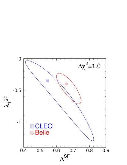
Figure 5: The fitted $\Delta\chi^{2}=1$ contours for CLEO (blue) and Belle (red) assuming an exponential shape function form.

V Summary

We have determined the $b$-quark shape function parameters, $\Lambda^{\mathrm{SF}}$ and $\lambda_{1}^{\mathrm{SF}}$, from fits of Monte Carlo simulated spectra to the raw Belle measured $B\rightarrow X_{s}\gamma$ photon energy spectrum. Raw refers to the spectrum as measured after the application of analysis cuts. We used three models for the form of the shape function; Exponential, Gaussian and Roman. We found the best fit parameters; $(\Lambda^{\mathrm{SF}},\lambda_{1}^{\mathrm{SF}})_{\mathrm{Exp}}=(0.66,-0.40)$, $(\Lambda^{\mathrm{SF}},\lambda_{1}^{\mathrm{SF}})_{\mathrm{Gauss}}=(0.63,-0.33)$, and $(\Lambda^{\mathrm{SF}},\lambda_{1}^{\mathrm{SF}})_{\mathrm{Roman}}=(0.66,-0.39)$, where $\Lambda^{\mathrm{SF}}$ and $\lambda_{1}^{\mathrm{SF}}$ are measured in units of $\mathrm{GeV}/c^{2}$ and $\mathrm{GeV}^{2}/c^{2}$ respectively. We also determined the $\Delta\chi^{2}=1$ contours in the $(\Lambda^{\mathrm{SF}},\lambda_{1}^{\mathrm{SF}})$ parameter space for each of the assumed models.

References

• (1) A. Bornheim et al. (CLEO Collaboration), Phys. Rev. Lett. 88, 231803 (2002).
• (2) B. Aubert et al. (BaBar Collaboration), Phys. Rev. Lett. 92, 071802 (2004).
• (3) H. Kakuno et al. (Belle Collaboration), Phys. Rev. Lett. 92, 101801 (2004).
• (4) F.D. Fazio and M. Neubert, J. High Energy Phys. 9906, 017 (1999).
• (5) M. Neubert, Phys. Rev. D 49, 3392 and 4623 (1994).
• (6) I. Bigi, M. Shifman, N. Uraltsev and A. Vainshtein, Int. J. Mod. Phys. A 9, 2467 (1994). R. Dickman, M. Shifman, and N. Uraltsev, Int. J. Mod. Phys. A 11, 571 (1996).
• (7) T. Mannel and M. Neubert, Phys. Rev. D 50, 2037 (1994).
• (8) I. Bigi, M. Shifman, N. Uraltsev and A. Vainstein, Phys. Lett. B328, 431 (1994).
• (9) A.L. Kagan and M. Neubert, Eur. Phys. J. C7 5 (1999).
• (10) L. Gibbons (CLEO Collaboration), hep-ex/0402009.
• (11) P. Koppenburg et al. (Belle Collaboration), hep-ex/0403004.
• (12) S. Anderson, Ph.D. thesis, University of Minnesota, 2002.
• (13) We thank R. Faccini for suggesting such a function.
• (14) D. Cronin-Hennessy, private communication.