Neutral Flavor Tagging for the Measurement of Mixing-induced Violation at Belle
Abstract
We describe a flavor tagging algorithm used in measurements of the violation parameter at the Belle experiment. Efficiencies and wrong tag fractions are evaluated using flavor-specific meson decays into hadronic and semileptonic modes. We achieve a total effective efficiency of .
keywords:
Flavor tagging , violation , , - mixingPACS:
29.85.+c , 07.05.Kf , 11.30.Er, , , , , , , , , , , , , , ,
1 Introduction
In the Standard Model (SM) of elementary particles, violation arises from an irreducible complex phase in the weak interaction quark-mixing matrix (CKM matrix) [1]. In particular, the SM predicts a -violating asymmetry in the time-dependent rates for and decays to a common eigenstate [2]. This -violating asymmetry in the dominated by the transition, has recently been observed by the Belle and BaBar groups [3, 5]. The measurement at Belle is based on a sample of pairs collected at the resonance at the KEKB asymmetric-energy collider. In the decay chain , where one of the two mesons decays at time to and the other, at time to a final state that distinguishes and , the decay rates and their asymmetry are time dependent. The time dependence for transitions is given by
| (1) | |||||
| (2) |
where represents the normalized decay rate, is the lifetime, is the CP-eigenvalue of , is the mass difference between the two mass eigenstates, = , the -flavor charge = +1 () when the tagging meson is a (). The parameter is one of the three interior angles of the CKM unitarity triangle, defined as . The eigenstates are reconstructed from , , , , , or decays.
An identification of the flavor of the accompanying meson, called flavor tagging in this article, is required to observe this kind of -violating asymmetry. A perfect tagging algorithm with a perfect detector will tag every meson that decays into a flavor specific decay mode and will identify the flavor of the meson. A practical tagging algorithm in a realistic detector will tag only a fraction (the tagging efficiency) of mesons and of those tagged, only a fraction of them will be identified correctly. The fraction of mesons identified incorrectly is called the wrong tag fraction . The observed time dependence thus becomes
| (3) | |||||
and the observed -violating asymmetry ,
| (4) | |||||
Here, we ignore a possible small difference between wrong tag fraction for and . The observed -violating asymmetry is diluted by , which is called the dilution factor. The statistical significance of the asymmetry measurement is proportional to , i.e. the number of events required to observe the asymmetry for a certain statistical significance is inversely proportional to , which is called the “effective tagging efficiency”. At the same time, since the the factor is proportional to the amplitude of observed -asymmetry, the wrong tag fraction directly affects the central value of . Therefore, a precise measurement of is crucial in order to minimize the systematic uncertainty in the measurement.
Our tagging algorithm has been developed to maximize while making it possible to determine the value of experimentally. The flavor tagging described in this paper is used not only for the measurement but also for other measurements such as measurements [18, 19] and measurements of -violating asymmetries in the decay [20]. In this paper, we present an algorithm for flavor tagging and describe its performance. The experimental apparatus of the Belle experiment is described in the next section. The flavor tagging algorithm is described in Section 3, and the measurement of its performance and wrong tag fractions with the control samples of self-tagged neutral decays, in Section 4.
2 Experimental Apparatus
The Belle experiment is conducted at the KEKB energy-asymmetric (3.5 GeV) (8.0 GeV) collider with a crossing angle of 22 mrad. The corresponding center-of-mass (CMS) energy is 10.58 , which is on the resonance. The decays into pairs with a Lorentz boost of nearly along the axis, which is defined as opposite to the positron beam direction. The time difference between the two meson decays is measured from the distance between the two decay vertices ().
The Belle detector [6] is a general-purpose spectrometer surrounding the interaction point. It consists of a barrel, forward and backward components. It is placed in such a way that the axis of the detector solenoid is parallel to the axis. In this way, the Lorentz force on the low energy positron beam is minimized.
Precision tracking and vertex measurements are provided by a central drift chamber (CDC) [7] and a silicon vertex detector (SVD) [8]. The CDC is a small-cell cylindrical drift chamber with 50 layers of anode wires including 18 layers of stereo wires. A low- gas mixture [He (50%) and (50%)] is used to minimize multiple Coulomb scattering and to ensure a good momentum resolution, especially for low momentum particles. It provides three-dimensional trajectories of charged particles in the polar angle region in the laboratory frame, where is measured with respect to the axis. The SVD consists of three layers of double-sided silicon strip detectors arranged in a barrel and covers 86% of the solid angle. The three layers at radii of 3.0, 4.5 and 6.0 cm surround the beam-pipe, a double-wall beryllium cylinder of 2.3 cm outer radius and 1 mm thickness. The strip pitches are 84 m for the measurement of coordinate and 25 m for the measurement of the azimuthal angle . The impact parameter resolution for reconstructed tracks is measured as a function of the track momentum (measured in GeV/c) to be = [19 50/()] m and = [36 42/()] m. The momentum resolution of the combined tracking system is %, where is the transverse momentum in GeV/c.
The identification of charged pions and kaons uses three detector systems: the CDC measurements of , a set of time-of-flight counters (TOF)[9] and a set of aerogel Čherenkov counters (ACC)[10]. The CDC measures energy loss for charged particles with a resolution of = 6.9% for minimum-ionizing pions. The TOF consists of 128 plastic scintillators viewed on both ends by fine-mesh photo-multipliers that operate stably in the 1.5 T magnetic field. Their time resolution is 95 ps () for minimum-ionizing particles, providing three standard deviation (3) separation below 1.0 GeV/, and 2 up to 1.5 GeV/. The ACC consists of 1188 aerogel blocks with refractive indices between 1.01 and 1.03 depending on the polar angle. Fine-mesh photo-multipliers detect the Čherenkov light. The effective number of photoelectrons is approximately 6 for particles. Using this information, , the probability for a particle to be a meson, is calculated. A selection with retains about 90% of the charged kaons with a charged pion misidentification rate of about 6%.
Photons are reconstructed in a CsI(Tl) crystal calorimeter (ECL) [11] consisting of 8736 crystal blocks, 16.1 radiation lengths () thick. Their energy resolution is 1.8% for photons above 3 GeV. The ECL covers the same angular region as the CDC. Electron identification [12] in Belle is based on a combination of measurements in the CDC, the response of the ACC, the position and the shape of the electromagnetic shower, as well as the ratio of the cluster energy to the particle momentum. The electron identification efficiency is determined from the two-photon processes to be more than 90% for GeV/. The hadron misidentification probability, determined using tagged pions from inclusive decays, is below .
All the detectors mentioned above are inside a super-conducting solenoid of 1.7 m radius that generates a 1.5 T magnetic field. The outermost spectrometer subsystem is a and muon detector (KLM)[13], which consists of 14 layers of iron absorber (4.7 cm thick) alternating with resistive plate counters (RPC). The KLM system covers polar angles between 20 and 155 degrees. Muon identification is based on the depth of penetrated KLM layers and the position matching from the CDC. The overall muon identification efficiency, determined by using the two-photon process and simulated muons embedded in candidate events, is greater than 90% for tracks with GeV/c detected in the CDC. The corresponding pion misidentification probability, determined using decays, is less than 2%.
3 Flavor Tagging Algorithm
3.1 Principle of Flavor Tagging
We determine the flavor of the accompanying meson based on the flavor information of the final state particles that belong to . Namely, the flavor of can be determined from the charge (flavor) of
-
1.
high-momentum leptons from decays,
-
2.
kaons, since the majority of them originate from decays through the cascade transition ,
-
3.
intermediate momentum leptons from decays,
-
4.
high momentum pions coming from decays,
-
5.
slow pions from decays, and
-
6.
baryons from the cascade decay .
The flavor tagging algorithm cannot always determine the flavor of the mesons from the final state particles; i.e. in general. This is caused by:
-
•
inefficiency in particle detection and identification,
-
•
flavor-nonspecific decay processes such as ,
-
•
processes that have very little information on -flavor such as , for which the charged particles in the final state are all pions.
The incorrect assignment of the flavor is mainly caused by
-
•
particle misidentification and
-
•
smaller physical processes that give a flavor estimate that is opposite to the dominant process, e.g. the charged kaon from the decay in processes.
To maximize , we need to maximize , and minimize using all available information for each event. As described in detail in the following subsections, a larger is obtained by treating events with large ’s and small ’s separately. For this purpose, we use an expected event-by-event dilution factor , which is described in detail in the next section. We first find a signature of the aforementioned flavor specific categories in each charged track and/or a baryon candidate in an event. We assign to each track/ candidate. We combine all such particle level ’s taking their correlations into account, and estimate the value for the event. We classify events into six regions according to their values. The value is determined using Monte Carlo (MC) simulation and is related to as if the MC simulates the data perfectly. For each region, we assign a wrong tag fraction , which is measured using the control data sample. The values of are used along with decay time information in an unbinned maximum likelihood fit to determine the asymmetry parameter .
3.2 Flavor Tagging Algorithm
We use two parameters, and , as the flavor tagging outputs. The parameter is the flavor of the tag-side , as defined in Section 1. The parameter is an expected flavor dilution factor that ranges from zero for no flavor information to unity for unambiguous flavor assignment . In order to obtain a high overall effective efficiency, we must assign the best estimated flavor dilution factor to each event. To best accomplish this, we use multiple discriminants in the event. Using a multi-dimensional look-up table binned by the values of the discriminants, the signed probability, , is given by
| (5) |
where and are the numbers of and in each bin of the look-up table prepared from a large statistics MC event sample. For example, consider a table with only one bin. The tagging efficiency and effective tagging efficiency can be written as
| (6) | |||||
| (7) |
If we subdivide this bin into two bins, the tagging efficiencies, flavor dilution factors and effective tagging efficiencies can be written as
| (8) | |||||
| (9) | |||||
| (10) |
Using and , the sum of the effective efficiencies of the two bins becomes
| (11) |
If , then the effective efficiency increases by subdividing. This can easily be generalized to the case of subdivision into bins. The increase of the effective tagging efficiency is proportional to the dispersion of the flavor dilution factor, and is always positive. The number of of bins is practically limited by the quality and quantity of the Monte Carlo simulation data sample. Therefore, bins with a large dispersion of and with sufficient Monte Carlo statistics are subdivided.
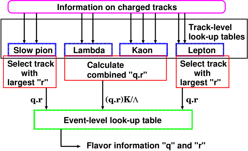
Figure 1 shows a schematic diagram of the flavor tagging method. The flavor tagging proceeds in two stages: the track stage and the event stage. In the track stage, each pair of oppositely charged tracks is examined to satisfy criteria for the -like particle category. The remaining charged tracks are sorted into slow-pion-like, lepton-like and kaon-like particle categories. The -flavor and its dilution factor of each particle, , in the four categories is estimated using discriminants such as track momentum, angle and particle identification information. In the second stage, the results from the first stage are combined to obtain the event-level value of .
In the Belle detector, there is a small asymmetry between particle and anti-particle production and detection. For example, the observed yields and signal-to-noise ratios of and candidates are different due to differences in interactions of the protons and anti-protons in the detector and differences in their yields in the background. In our method, and are treated separately and the effect of the small charge asymmetry is automatically taken into account. The candidates have higher tagging efficiency than candidates due to the larger yields of protons in the background. On the other hand, for ’s is lower than for ’s as the look-up table for ’s contains larger backgrounds that are generated correctly in the MC simulation. For other tagging categories such as lepton-, kaon- and slow-pion-like tracks, there are also small asymmetries, which are treated in the same way as candidates.
Using the MC-determined flavor dilution factor as a measure of the tagging quality is a straightforward and powerful way of taking into account correlations among various tagging discriminants. Using two stages, we keep the look-up tables small enough to provide sufficient MC statistics for each bin. In the following we provide details about each stage of the flavor tagging. Four million MC events corresponding to eight million ’s are used to generate the particle-level look-up tables. To reduce statistical fluctuations of the values in the particle-level look-up tables, the value in each bin is calculated by including events in nearby bins with small weights. The event-level look-up table is prepared using MC samples that are statistically independent of those used to generate the track-level tables to avoid any bias from a statistical correlation between the two stages. Seven million MC events corresponding to fourteen million ’s are used to create the event-level look-up table. We use GEANT3[14] to fully simulate the detector. Two event generators, QQ[15] and EvtGen[16], are used to simulate the tag-side meson decays. We used QQ-generated MC for early measurements of [3, 4] and EvtGen-generated MC for more recent measurements [17].
3.3 Particle-level Flavor Tagging
For the particle-level flavor tagging, charged tracks that do not belong to and that satisfy the impact parameter requirements cm and cm are considered. To find and candidates, we also use pairs of oppositely charged tracks that do not belong to according to a secondary vertex reconstruction algorithm. Tracks that are a part of a candidate or a candidate are not used. However, the number of ’s in the event is used as a discriminant in the -like and kaon-like particle categories.
3.3.1 Electron-like and Muon-like Track Categories
A track is assigned to the electron-like track category if the CMS momentum is larger than 0.4 GeV/ and the ratio of its electron and kaon likelihoods is larger than 0.8. A track is passed to the muon-like track category if the track has larger than 0.8 GeV/ and the ratio of its muon and kaon likelihoods is larger than 0.95. The likelihoods are calculated by combining the ACC, TOF, , and ECL or KLM information.
The discriminants for lepton-like track categories are summarized in Table 1. The charge of the particle provides the -flavor , and other discriminants determine its quality . The identifier “ or ” specifies whether a track belongs to the electron-like or the muon-like track categories. The lepton identification is optimized to reduce the kaon contamination, while a substantial fraction of pions is included in the muon-like track category. Prompt pions from the virtual decay sometimes preserve the charge (flavor) of the boson and therefore can be used to identify the flavor of the meson. About a half of such pions are included in the muon-like track categories and the rest, in the kaon-like track category. Such pions in the muon-like track category are included in the bins with low lepton ID probability and with high momentum.
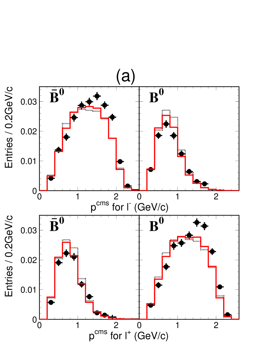
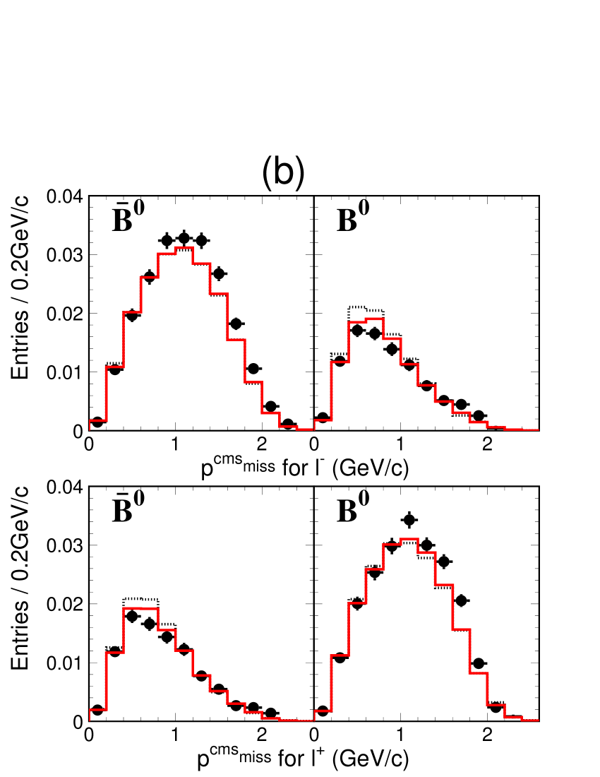
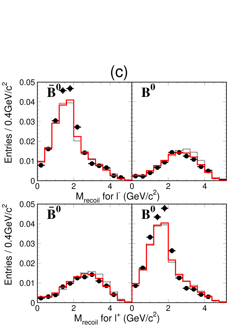
The variables and are used to subdivide the table as the purity and the efficiency of the lepton identification vary as a function of these variables. The requirement is also set to accept most of the primary leptons from the decays but includes some contamination due to secondary leptons from decays. Since the leptons from cascade decays give an incorrect flavor assignment, separation from the primary leptons in decay is important. The variable discriminates primary leptons that tend to have higher momenta. The variables and are calculated using all the observed charged and neutral particles that do not belong to . A neutrino from semileptonic decay carries away more momentum than one from a semileptonic decays. The distribution for semileptonic decays peaks around the mass and has a tail toward the lower side due to missing particles, while the one for semileptonic decay distributes widely up to 5 since is calculated including the decay products of the primary meson.
Figure 2 shows the , and distributions for the data and the MC. Although some disagreement is visible, the experimental bias due to this disagreement is found to be negligible since is evaluated from control samples as described in Section 4.
Within the lepton categories, leptons from semileptonic decays yield the highest effective efficiency while leptons from cascade decays and high-momentum pions from make small additional contributions.
3.3.2 Slow-pion-like Track Category
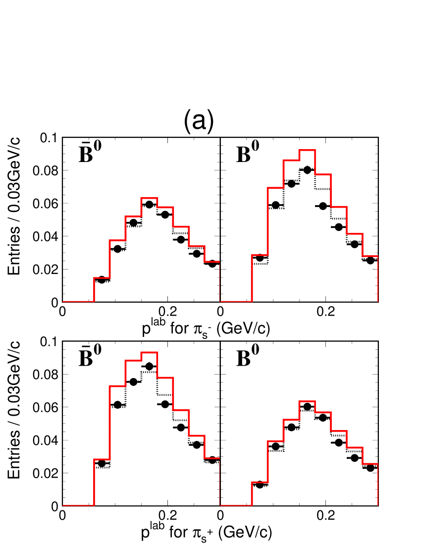
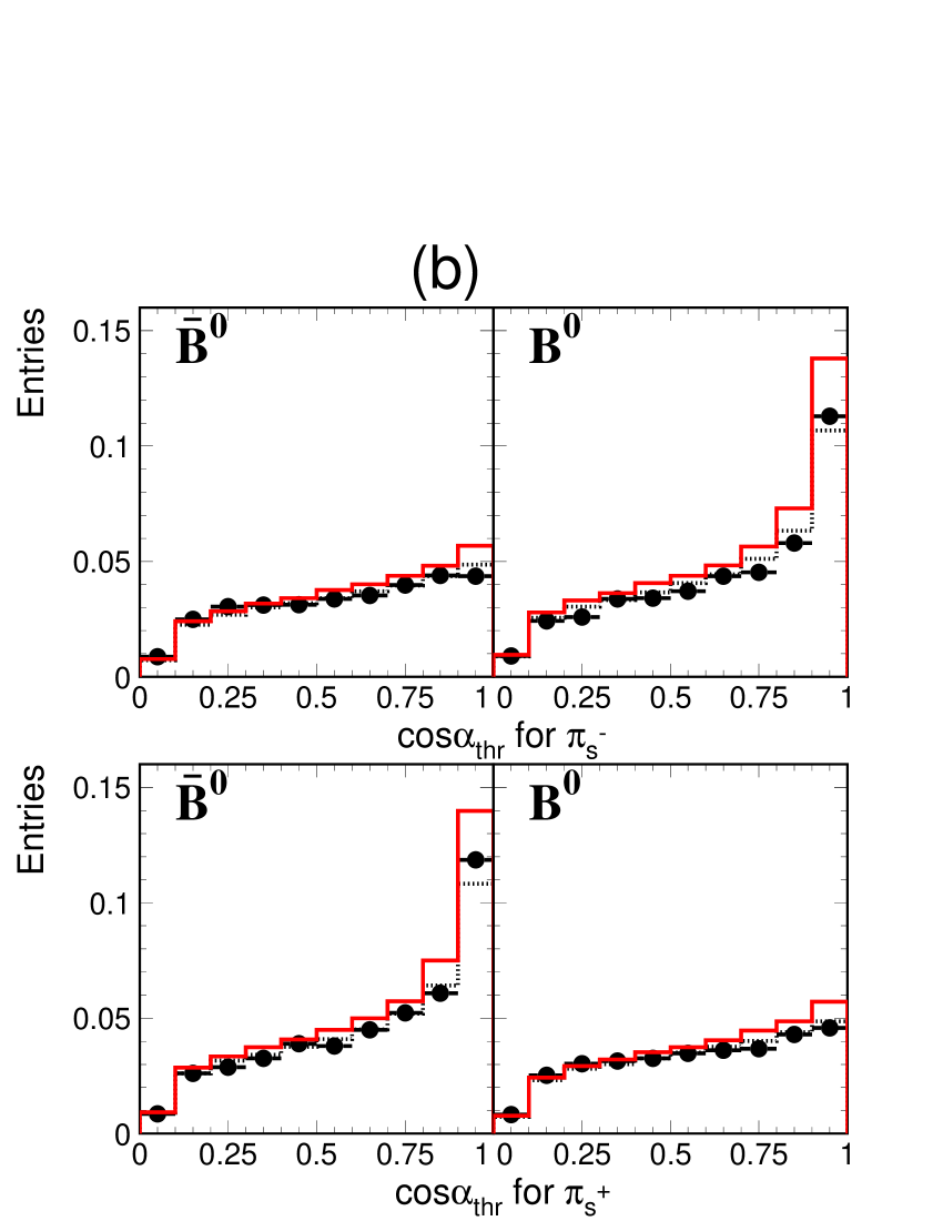
A track that has CMS momentum below 0.25 GeV/ and is not identified as a kaon, is assigned to the slow-pion-like track category. The discriminant variables for the slow-pion-like track category are given in Table 2. The largest background is from other (i.e. non- daughter) low momentum pions. Since the value is small, the pion from the decay has a low momentum and has a flight direction that follows the direction. We use , the angle between the direction of the slow-pion-like track and the axis of the thrust calculated from the tag-side particles in the CMS to select decays.
The other background in this category is from electrons produced in photon conversions and Dalitz decays. Electrons coming from photon conversion are identified through the secondary vertex reconstruction algorithm and are rejected. To separate slow pions from the remaining electrons, we use only because the tracks do not have enough transverse momenta () to reach the ECL detector, which gives and other useful information to discriminate electrons from pions. The ID probability from strongly depends on the laboratory momentum; the losses are equal for electrons and pions around . Thus, we use instead of in this category. Figure 3 shows the distribution of and the momenta of the slow pion candidates in the laboratory frame, which are uniquely determined by the values of and .
3.3.3 Kaon-like Track Category
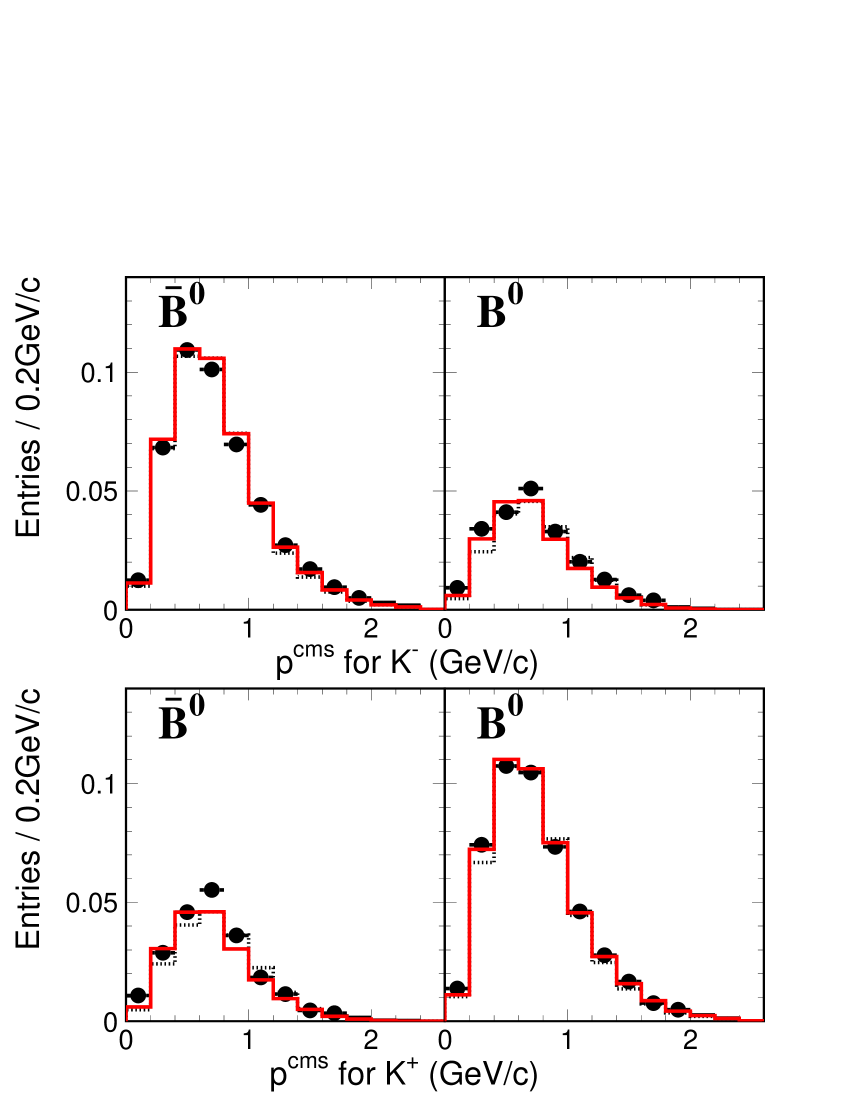
If a track does not fall into any of the categories described above, and is not positively identified as a proton, it is classified as a kaon-like track. Charged kaons from are included into this category. Some pions are also included in this category. The discriminants for this category are listed in Table 3. The variables , and ID separate kaons from pions. For identification, the information from the , TOF and ACC detectors is combined into a likelihood variable and a single kaon probability is calculated. The table is subdivided into and bins as the purity of kaon changes as a function of these variables.
The kaon-like track category is subdivided into two parts: events with and without decays (a switch “w/ or w/o ”), since they have different purities; a kaon accompanied with ’s tends to originate from a strange quark in a decay or from popping, while one without ’s has a higher probability to be from the cascade decay ().
The bins for low kaon probability and high contain fast pions. Fast pions from a prompt decay, such as , have flavor information and give some contribution to . Figure 4 shows the CMS momentum distribution of kaon-like track candidates compared to those in MC.
3.3.4 -like Particle Category
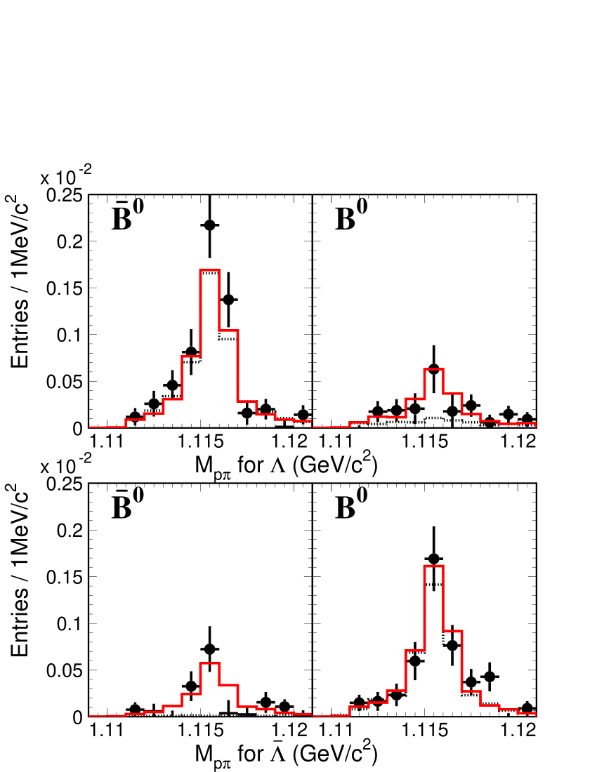
candidates are selected from pairs of oppositely-charged tracks one of which is identified as proton, and that also satisfy , , cm and with a secondary vertex position in the plane above 0.5 cm. Figure 5 shows the distributions for the data and the MC. The discriminants for this category as well as the definitions of , and are listed in Table 4. The last column is the number of bins for the corresponding discriminant.
As the purity (signal-to-noise ratio) of the candidates varies as a function of the variables , , and , we subdivide this category using these variables. Since the number of candidates is small, for each discriminant we subdivide into two (high and low quality) bins. The high quality bin contains candidates with , and cm.
3.4 Event-level Flavor Tagging
The track-level ’s are combined for event-level tagging. From the lepton-like and slow-pion-like track categories, the track with the highest -value from each category is chosen as the input to the event level look-up table. The flavor dilution factors of the kaon-like and -like particle candidates are combined by calculating the product of the flavor dilution factors in order to account for the cases with multiple quark contents in an event. The product of flavor dilution factors gives better effective efficiency than taking the track with the highest . Table 5 shows the discriminants for event-level tagging. By using a three-dimensional look-up table, the correlations between flavor information for lepton-like, slow-pion-like, kaon-like and -like particles are correctly taken into account. In the event-level look-up table, one of the bins in Table 5 corresponds to “empty” for the case when there is no output from a particular particle-level category.
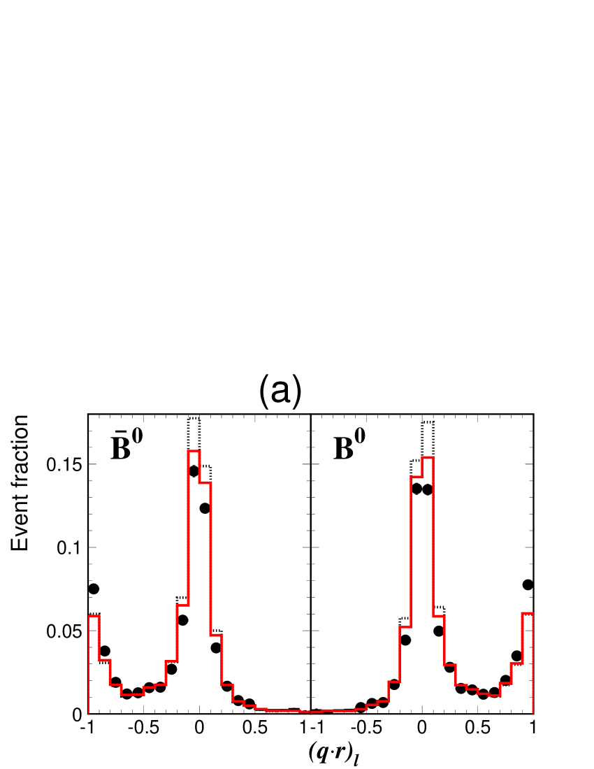
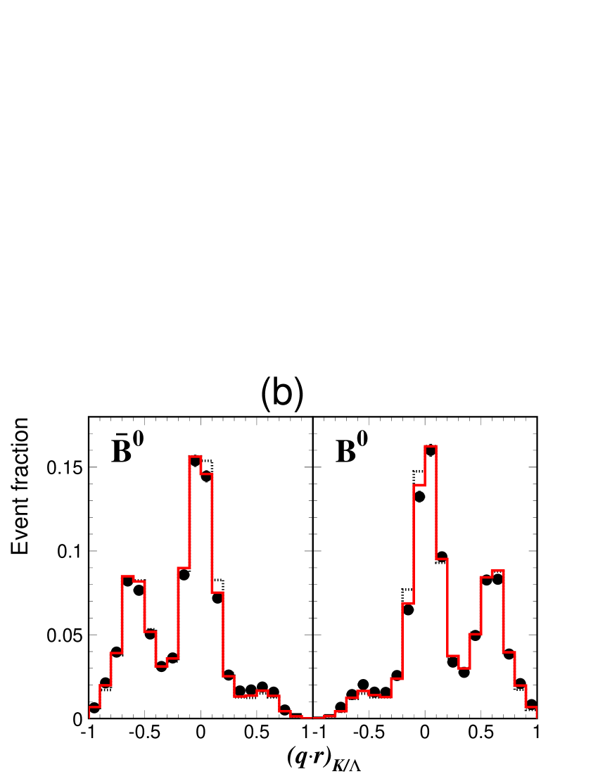
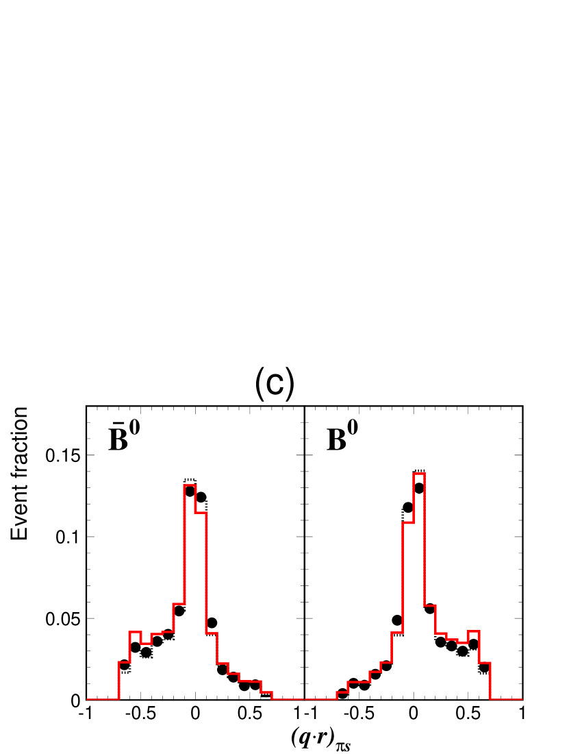
Figure 6 shows the distributions of input values for the event layer. The distribution of has peaks around due to the high momentum primary leptons from semileptonic decays. The effective efficiency for the lepton category is 12% according to MC simulation. The distribution of has peaks around , which correspond to events with a single kaon or a candidate. The entries around correspond to events with multiple kaon and/or candidates with consistent flavor information. Kaons have higher yields but less flavor information compared to leptons. The combined effective efficiency estimated for kaon and categories is 18% according to MC. The distribution of contains no entries beyond , as the slow-pion-like track category has much more background than other categories. The effective efficiency for the slow-pion-like track category is estimated to be 6% according to MC. The peaks around zero in the three distributions are due to pions that have little flavor information.
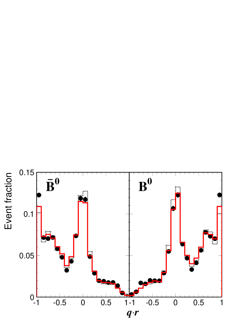
The probability that we can assign a non-zero value for is 99.6% according to MC; i.e. almost all the reconstructed candidates can be used to extract . Using a MC sample that is statistically independent of those used to generate the look-up tables, we estimate the effective efficiency to be . Since the lepton-like, kaon/-like and slow-pion-like particle tagging categories are not exclusive, the effective tagging efficiency is smaller than the sum of the efficiencies for the individual particle categories. We compare the distribution of obtained from the control data samples with the MC expectation. As shown in Figure 7, the data and MC are in good agreement.
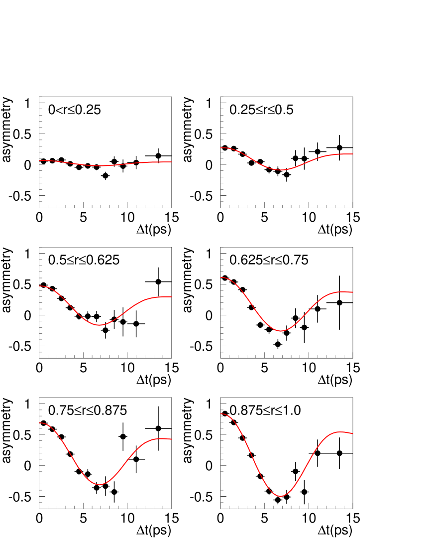
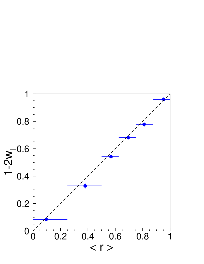
Finally, we obtain the wrong tag fraction, for each event from the MC-determined event-level flavor dilution factor, . Trusting the Monte Carlo simulation completely we could assign for each event from the relation, . However, using the method described in the following section, we measure using the control data samples of flavor specific decays and use the measured values in the unbinned maximum likelihood fit to extract . All tagged events are sorted into six subsamples according to the value of ; , , , , and . Wrong tag fractions are measured for the six regions. The average value of for each region () and measured wrong tag fraction () should satisfy , if the MC that is used for constructing the look-up tables simulates generic decays correctly. Using the measured (and therefore average) value for the region instead of a value calculated for each event from MC, we introduce no systematic bias into the measurement of from the Monte Carlo simulation, although the effective tagging efficiency degrades. The degradation from the subdivision into bins is estimated to be about , according to a Monte Carlo study. Nevertheless, in such a categorization based on the value, we can achieve a higher effective tagging efficiency than using the traditional method of treating lepton, kaon and slow pion tags separately; by using a conventional tagging method with kaons and high momentum leptons, we obtain an total effective tagging efficiency of .
We have also investigated the dependence of flavor tagging performance on MC. We prepared two sets of lookup tables, a QQ-generated table and a EvtGen-generated table. Comparing the QQ-generated and the EvtGen-generated tables, we find the EvtGen-generated table has the larger effective tagging efficiency. As a result, we switched to EvtGen-MC tables starting with the updated analysis [17]. In this section, the performance of the flavor tagging with EvtGen-MC is discussed and that with QQ-MC is referred to for comparison purposes only. The performance of the latter is described in [4].
4 Flavor Tagging Performance
The flavor tagging performance is evaluated using the control samples of self-tagged -meson decays, which are described in Appendix A. The flavor tagging efficiency, is measured to be 99.8%, which is consistent with the MC expectation. The wrong tag fraction is obtained by fitting the time-dependent - mixing oscillation signal. The analysis method is similar to the one used in the previous Belle - mixing analysis [18, 19]. The time evolution of neutral -meson pairs with opposite flavor (OF) or same flavor (SF) is given by:
| (12) |
and the OF-SF asymmetry,
| (13) |
We obtain the wrong tag fraction using an unbinned maximum likelihood fit to the reconstructed distribution of the SF and OF events with and fixed to the world average values [22]. The likelihood function is defined as:
| (14) |
where the index runs over all selected OF(SF) events. The function is the sum of signal probability density function smeared by the resolution and the background component, written as:
where and are the signal fraction and the background shape, respectively, whose description can be found elsewhere [18, 19], and is the resolution function. A small fraction of events at large (outliers) are represented by a Gaussian of a large width, . The outlier-fraction , the width of and the resolution function are determined in the lifetime analysis [21].
Figure 8 shows the measured OF-SF asymmetries as a function of . Figure 9 shows the measured vs. , which confirms the validity of our tagging method.
The fit results are summarized in Table 6. We also evaluate the wrong tag fractions for -tagged events and -tagged samples separately as a check, since they can be different due to charge asymmetries in the particle identification and proton fakes in candidates. The values for the two samples are listed in Table 7. We will use separate for -tagged and -tagged samples as the statistics of the control samples increases. 111 The latest update of based on a data sample of pairs uses separate values for -tagged and tagged samples.
Systematic errors are summarized in Table 8. The uncertainties in semileptonic modes are the dominant components. The systematic errors due to the uncertainty of the signal fraction are estimated by changing each fraction or parameter representing the fraction by , repeating the fit and adding the deviations from the main result in quadrature. For the hadronic modes, we consider the effect of changing the signal region in the energy difference by 10 MeV and beam-energy constrained mass by 3MeV, where and are the energy and the momentum of the reconstructed meson in the center of mass system. Each parameter in the background shape is varied by , the fit is repeated and the errors are added in quadrature. We also check a possible difference between the background shape in the signal region and the background control sample using MC simulation and include it in the systematic error. We use MC to estimate the background in the semileptonic sample, where denotes non-resonant and heavier charmed mesons. We evaluate the systematic errors due to uncertainties of the branching fractions of each component by successively setting each component in turn to unity in the MC (with all others set to zero), and repeating the fit. We take the largest variation in as the systematic error. The effect of the uncertainty in the background for the semileptonic mode is also included. Systematic errors originating from the vertex reconstruction are estimated by modifying the vertex quality and track quality selection for the tagging side by and by varying the flight length assumed in the interaction point constraint by m. We also check the result with different ranges, 40 ps or 100 ps instead of the nominal range of 70 ps. The resolution function uncertainty is obtained by modifying each parameter in the resolution function by . The dependence on the lifetime and the is measured by varying the measured values by . We test for a bias in a reconstruction with large statistics signal MC samples and observe no statistically significant discrepancy, therefore no systematic error due to reconstruction bias is included.
The total effective efficiency obtained by summing over the six regions is
where is the event fraction in each of the six regions. The error includes both statistical and systematic contributions.
5 Summary
We have developed a flavor tagging algorithm for the measurement of the violation parameter and other measurements at the Belle experiment. The algorithm is designed to maximize the effective tagging efficiency, , where is the efficiency and is the wrong tag fraction. We introduce two variables and , where is the flavor charge of a meson and is the MC-determined event-by-event flavor dilution factor. The value is related to through . In our approach, we independently determine from control data samples, which are self-tagging events and check the relation, . We therefore avoid possible biases that may be introduced by the use of MC. We have achieved an effective efficiency of according to MC simulation, which is significant improvement over the value of achieved by the classical method of flavor tagging using only leptons and kaons.
The flavor tagging performance is estimated from samples of decays into the self-tagged modes, and . A total of 65332 events are used to evaluate the performance. We obtain an effective tagging efficiency of ()%, which agrees well with the MC expectation.
Acknowledgments
We would like to thank the members of the Belle collaboration. We especially acknowledge those who calibrate the tracking and the particle identification devices of the Belle detector. We are grateful to T. E. Browder for a careful reading of the manuscript. This work was supported in part by Grant-in-Aid for Scientific Research on Priority Areas (Physics of violation) from Ministry of Education, Culture, Sports, Science and Technology of Japan.
| variable | description | number of bins |
|---|---|---|
| charge | track charge | 2 |
| or | identifier of an electron or muon | 2 |
| lepton ID | lepton-ID quality value | 4 |
| the magnitude of the momentum in the CMS | 11 | |
| the polar angle in the laboratory frame | 6 | |
| the hadronic recoil mass | 10 | |
| the magnitude of the missing momentum in the CMS | 6 | |
| total | 31680 |
| variable | description | number of bins |
|---|---|---|
| charge | track charge | 2 |
| the magnitude of the momentum in the laboratory frame | 10 | |
| the polar angle in the laboratory frame | 10 | |
| the cosine of the angle between the slow pion candidate and the thrust axis of the tag-side particles in the CMS | 7 | |
| ID | pion ID probability from | 5 |
| total | 7000 |
| variable | description | number of bins |
|---|---|---|
| charge | Track charge | 2 |
| w/ or w/o | switch to indicate whether the event contain ’s or not | 2 |
| momentum in the center-of-mass system of | 21 | |
| polar angle in the laboratory system | 18 | |
| ID | quality value of ID(, TOF, ACC) | 13 |
| total | 19656 |
| variable | description | number of bins |
|---|---|---|
| flavor | flavor of ( or ) | 2 |
| presence | switch that indicates whether the event contains ’s or not | 2 |
| invariant mass of the pion and the proton candidate at the secondary vertex | 2 | |
| the angle difference between the momentum vector and the direction of the vertex point from the nominal IP | 2 | |
| difference of the two tracks at the vertex point | 2 | |
| total | 32 |
| variable | description | number of bins |
|---|---|---|
| for the highest from outputs of lepton category | 25 | |
| from the product of likelihood; where the subscript runs over all outputs of the kaon and categories. | 35 | |
| for the highest from outputs of slow pion category | 19 | |
| total | 16625 |
| interval | ||||
|---|---|---|---|---|
| 1 | 0.000 – 0.250 | 0.398 | ||
| 2 | 0.250 – 0.500 | 0.146 | ||
| 3 | 0.500 – 0.625 | 0.104 | ||
| 4 | 0.625 – 0.750 | 0.122 | ||
| 5 | 0.750 – 0.875 | 0.094 | ||
| 6 | 0.875 – 1.000 | 0.136 |
| interval | for | for | |
|---|---|---|---|
| 1 | 0.000 – 0.250 | ||
| 2 | 0.250 – 0.500 | ||
| 3 | 0.500 – 0.625 | ||
| 4 | 0.625 – 0.750 | ||
| 5 | 0.750 – 0.875 | ||
| 6 | 0.875 – 1.000 |
| source | ||||||
|---|---|---|---|---|---|---|
| Semileptonic signal fraction | ||||||
| Semileptonic background shape | ||||||
| Semileptonic composition | ||||||
| Semileptonic background | ||||||
| Hadronic signal fraction | ||||||
| Hadronic background shape | ||||||
| Hadronic background mixing | ||||||
| Vertex reconstruction | ||||||
| Resolution parameters | ||||||
| lifetime and | ||||||
| Total |
Appendix A Control Samples for Flavor Tagging
Control samples of self-tagged -mesons are used to measure ’s directly from data, and minimize the systematic uncertainty in our measurement. The control samples are also used for the evaluation of the flavor tagging performance and to check flavor tagging inputs and outputs. We use the semileptonic decay mode, [18] and hadronic modes , and [19] and their charge conjugates as control samples. We fully reconstruct those -meson decays and tag the -flavor of the associated -mesons using the algorithm described in Section 3. Using the 78 fb-1 data sample corresponding to pairs, we select 47317 semileptonic decay candidates with 79.2% purity and 18015 hadronic decay candidates with purities of 87.9%, 84.3% and 72.6% for the , and modes, respectively. In the measurement and evaluation described in Section 4, the effect of - mixing is taken into account by fitting the time dependence of the flavor mixing. For the figures that show flavor tagging input variables and outputs in Section 3, we use [22] to take the effect of mixing into account. In those figures, the number of entries in an event for () is calculated as , where and are the entries and the total number of events from the background subtracted () control samples, respectively, and and are those from the background subtracted () control samples.
References
- [1] M. Kobayashi and T. Maskawa, Prog. Theor. Phys. 49, 652 (1973).
- [2] A. B. Carter and A. I. Sanda, Phys. Rev. D 23, 1567 (1981); I. I. Bigi and A. I. Sanda, Nucl. Phys. B193, 85 (1981).
- [3] K. Abe et al. (Belle Collab.), Phys. Rev. Lett. 87, 091802 (2001)
- [4] K. Abe et al. (Belle Collab.), Phys. Rev. D 66, 032007 (2002).
- [5] B. Aubert et al. (BaBar Collab.), Phys. Rev. Lett. 87, 091801 (2001); B. Aubert et al. (BaBar Collab.), Phys. Rev. D 66, 032003 (2002).
- [6] A. Abashian et al.(Belle Collab.), Nucl. Inst. and Meth. A 479, 117 (2002).
- [7] H. Hirano et al., Nucl. Instr. and Meth. A 455, 294 (2000); M. Akatsu et al., Nucl. Instr. and Meth. A 454, 322 (2000).
- [8] G. Alimonti et al., Nucl. Instr. and Meth. A 453, 71 (2000).
- [9] H. Kichimi et al., Nucl. Instr. and Meth. A 453, 315 (2000).
- [10] T. Iijima et al., Nucl. Instr. and Meth. A 453, 321 (2000).
- [11] H. Ikeda et al., Nucl. Instr. and Meth. A 441, 401 (2000).
- [12] K. Hanagaki et al., Nucl. Instr. and Meth. A 485, 490 (2002).
- [13] A. Abashian et al., Nucl. Instr. and Meth. A 449, 112 (2000).
- [14] R. Brun et al., GEANT 3.21, CERN Report DD/EE/84-1, 1984.
-
[15]
The QQ meson decay event generator was developed by the CLEO
Collaboration (see
http://www.lns.cornell.edu/public/CLEO/soft/QQ). - [16] D. J. Lange, Nucl. Instr. and Meth. A 462, 152 (2001).
- [17] K. Abe et al. (Belle Collab.), Phys. Rev. D 66, 071102(R) (2002).
- [18] K. Hara et al. (Belle Collab.), Phys. Rev. Lett. 89, 251803 (2002).
- [19] T. Tomura et al. (Belle Collab.), Phys. Lett. B 542, 207 (2002).
- [20] K. Abe et al. (Belle Collab.), Phys. Rev. D 68, 012001 (2003), updated by K. Abe et al. (Belle Collab.), hep-ex/0401029, submitted to Phys. Rev. Lett.
- [21] K. Abe et al. (Belle Collab.), Phys. Rev. Lett. 88, 171801 (2002).
- [22] K. Hagiwara et al. (Particle Data Group), Phys. Rev. D 66, 010001 (2002).