Investigation of top mass measurements with the ATLAS detector at LHC

Abstract.

Several methods for the determination of the mass of the top quark with the ATLAS detector at the LHC are presented. All dominant decay channels of the top quark can be explored. The measurements are in most cases dominated by systematic uncertainties. New methods have been developed to control those related to the detector. The results indicate that a total error on the top mass at the level of 1 GeV should be achievable.

1 Introduction

A precise measurement of the top quark mass will be a main goal of top physics at the LHC. The combined top mass value from the Tevatron run I is $m_{t}=174.3\pm 5.1$ GeV [1], and the expected accuracy obtained after run II will be 3 GeV [2].

Motivations for an accurate determination of the top quark mass are numerous. It is a fundamental parameter of the Standard Model (SM) and should therefore be measured as precisely as possible. An accurate value of the top mass would help to provide a rigorous consistency check of the SM and to constrain some parameters of the model such as the mass of the Higgs boson. Furthermore, a high level of accuracy on the top mass value (for example improving the accuracy down to $\mathchar 257\relax m_{t}\sim 1$ GeV) is also desirable, both within the SM and the Minimal Supersymetric Standard Model (MSSM) framework [3]. In the SM, such an accuracy would significantly improve the precision on the W boson mass prediction while in the MSSM, it would put constraints on the parameters of the scalar top sector and would therefore allow sensitive test of the model by comparing predictions with direct observations.

Because the top quark, as other quarks, cannot be observed as a free particle, the top quark mass is a purely theoretical notion and depends on the concept adopted for its definition. With increasingly-precise measurements on the horizon, it is important to have a firm grasp of exactly what is meant by the top quark mass. Thus far the top quark mass has been experimentally defined by the position of the peak in the invariant mass distribution of the top quark’s decay products, a W boson and a b quark jet. This closely corresponds to the pole mass of the top quark, defined as the real part of the pole in the top quark propagator.

The renormalisation scale dependence is less than 10 MeV for the range of the scale between 30-150 GeV. The dominant theoretical uncertainty for the top mass caused by uncertainty on the strong coupling constant is less than 150 MeV to the binding energy, which would give uncertainty of 75 MeV in the pole mass. Corresponding theoretical uncertainty in the $\overline{MS}$ mass would be about $\pm$12 MeV[4]. However, this definition is still adequate for the analysis of top quark production at LHC where uncertainty in the top mass measurement will be of order 1 GeV. Because of fragmentation effects it is believed that the top quark mass determination in an hadronic environment is inherently uncertain to $\cal O(\mathchar 259\relax_{QCD})$ [3][5].

At the LHC, the top quark will be produced mainly in pairs through the hard process $gg\rightarrow t\bar{t}$ ($90\%$ of the total $t\bar{t}$ cross-section) and $q\bar{q}\rightarrow t\bar{t}$ (remaining $10\%$ of the cross-section). The next-to-leading order cross-section prediction for $t\bar{t}$ production is $\sigma(t\bar{t})=833$ pb [6]. Thus the LHC will be a top factory as more than 8 million $t\bar{t}$ pairs will be produced per year at low luminosity (corresponding to an integrated luminosity of $10\ \rm fb^{-1}$). The electroweak single top production processes, whose cross-sections are in total approximately one third of those of $t\bar{t}$ production, have not been investigated for the determination of the top mass.

Within the SM, the top quark decays almost exclusively into a W boson and a b-quark ($t\rightarrow Wb$). Depending on the decay mode of the W bosons the $t\bar{t}$ events can be classified into three channels: the lepton plus jets channel, the dilepton channel and the all jets channel. In the lepton plus jets channel, one of the W boson decays leptonically ($W\rightarrow l\nu$) and the other one hadronically ($W\rightarrow jj$). Considering electrons and muons, the branching ratio is $\rm BR=2\times 2/9\times 6/9\simeq 30\%$. The final state topology is $gg\rightarrow t\bar{t}\rightarrow(jjb)(l\nu b)$. In the dilepton channel, both W bosons decay leptonically with $\rm BR=2/9\times 2/9\simeq 5\%$. In the all jets channel, both W bosons decay hadronically with $\rm BR=6/9\times 6/9\simeq 44\%$.

This paper summarizes studies of the top mass measurement, including updates of studies presented in the ATLAS Technical Design Report [7] as well as several new analysis.

Unless otherwise indicated, all analysis were performed with events generated with Pythia [8] and passed through the ATLAS fast simulation package Atlfast [9] for particles and jets reconstruction and momenta smearing. Jets are defined as massless objects by summing the momenta of clusters of energy deposited in the calorimeters. Clusters are associated to form jets using a cone algorithm with $\delta(R)<0.4$. A tagging efficiency of 60% for b-jets was assumed. Cross-checks of some results have been made using the detailed GEANT-based simulation of the ATLAS detector. The top mass is extracted by an analytic fit to the event by event reconstructed invariant mass.

2 Top mass measurement in the lepton plus jets channel

The lepton plus jets channel is probably the most promising channel for an accurate determination of the top quark mass. Three methods to measure the top mass are envisaged. The simplest method consists in extracting the top mass from the three jets invariant mass of the hadronic top decay. In the second method, the entire $t\bar{t}$ system is fully exploited to determine the top quark mass from a kinematic fit. In the last method, the top mass is still determined from a kinematic fit, but the jets are reconstructed using a continuous algorithm.

2.1 Event selection and background rejection

Taking into account the total $t\bar{t}$ cross-section and the branching ratio, one can expect 2.5 millions $t\bar{t}$ pairs with this topology to be produced per year assuming an integrated luminosity $10fb^{-1}$.

The signal final state $t\bar{t}\rightarrow Wb\ Wb\rightarrow jjb\ l\nu b$ (with $l=e,\mu$) is characterized by one high transverse momentum lepton, large transverse missing energy $E_{T}^{miss}$, and high jet multiplicity. The following background processes were considered: $b\bar{b}\rightarrow l\nu+jets$, $W+jets\rightarrow l\nu+jets$, $Z+jets\rightarrow l^{+}l^{-}+jets$, $WW\rightarrow l\nu+jets$, $WZ\rightarrow l\nu+jets$, and $ZZ\rightarrow l^{+}l^{-}+jets$. At production level, the signal over background ratio is very unfavorable (S/B $\sim 10^{-5}$).

Process	Cross-section	Total efficiency
	(pb)	($\%$)
$t\bar{t}$ signal	250	3.5
$b\bar{b}\rightarrow l\nu+jets$	$2.2\times 10^{6}$	$3\times 10^{-8}$
$W+jets\rightarrow l\nu+jets$	$7.8\times 10^{3}$	$2\times 10^{-4}$
$Z+jets\rightarrow l^{+}l^{-}+jets$	$1.2\times 10^{3}$	$6\times 10^{-5}$
$WW\rightarrow l\nu+jets$	17.1	$7\times 10^{-3}$
$WZ\rightarrow l\nu+jets$	3.4	$1\times 10^{-2}$
$ZZ\rightarrow l^{+}l^{-}+jets$	9.2	$3\times 10^{-3}$

Table 1.: Cross-section and selection efficiency for signal and background processes. For the background, the hard scattering processes are generated with a cut on the transverse momentum at 20 GeV

A high level of rejection was obtained using the following requirements: one isolated lepton with $p_{T}>20$ GeV, $E_{T}^{miss}>20$ GeV, and at least four jets reconstructed with a cone size of $\mathchar 257\relax R=0.4$ with $p_{T}>40$ GeV and $|\eta|<2.5$, of which at least two are tagged as b-jets. The efficiency of the selection for the various background processes is shown in table 1. After selection cuts, the signal over background ratio is extremely good (S/B $\sim 78$), and the remaining number of signal events is approximately 87000 (for an integrated luminosity of $10^{-1}$fb).

Fig. 1.: $t\bar{t}$ sample as a function of the number of b-tagged jets in the event.

The requirement of having at least two b-tagged jets in the final state helps in rejecting a large part of the physical background, but also reduces considerably the signal sample. The fraction of signal events with at least two b-tagged jets is three times smaller than the fraction with at least one b-tagged jet (see figure 1). Requiring only one b-tagged jet would decrease the signal over background ratio from 78 to 28, which would still be acceptable. This extended sample can be used for the top mass measurement using the hadronic top decay, requiring the tagged b-jet to be the one belonging to the hadronic top final state.

2.2 Top mass measurement using the hadronic top decay

In the following method, the top mass will be determined from the invariant mass of the three jets arising from the hadronic top decay ($t\rightarrow Wb\rightarrow jjb$). To accurately reconstruct the decay, one should: i) identify the jets associated to the hadronic top decay among all other jets, ii) precisely calibrate the jet energies and directions.

2.2.1 Jet association

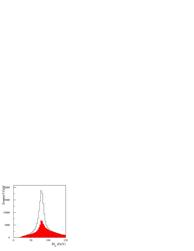
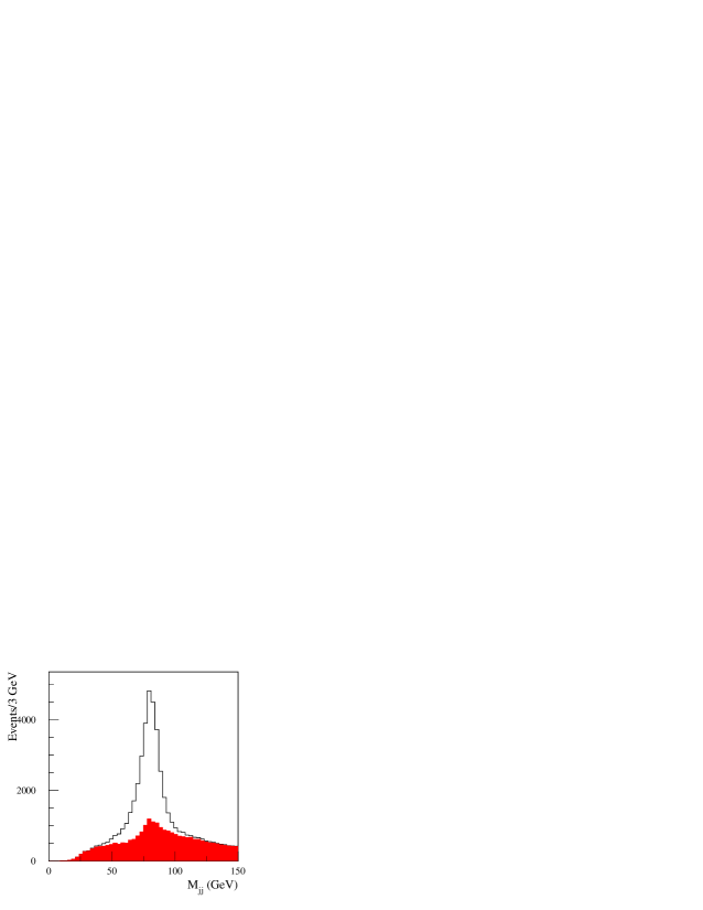
Fig. 2.: Dijet invariant mass distributions for events with at least 1 b-tagged jet (left plot), and at least 2 b-tagged jets (right plot). The shaded area represents the combinatorial background. Both plots are for 10 fb^-1.

At least four jets are expected in the event: two from the hadronic W decay and two b-jets. Additional jets will be produced by initial state radiation (ISR) and final state radiation (FSR) effects. The association of jets to the original partons is done as follows. The hadronic W decay is first reconstructed: all the non b-tagged jets are paired together and the jet pair with an invariant mass closest to the W mass is taken as the right combination for the W. The di-jet invariant mass distributions for events selected by requiring two b-tagged jets or at least one are shown on figure 2. When the two associated jets are reconstructed, 80 $\%$ of the true W decays are selected, which is realized in 45 $\%$ of the cases. This leads, in a mass window $|M_{jj}-M_{W}^{PDG}|<20$ GeV, to a purity of 55 $\%$ for events selected with at least one b-tagged jet and 66 $\%$ for events selected with two b-tagged jets. The width of the mass distribution is 7.4 GeV for both cases.

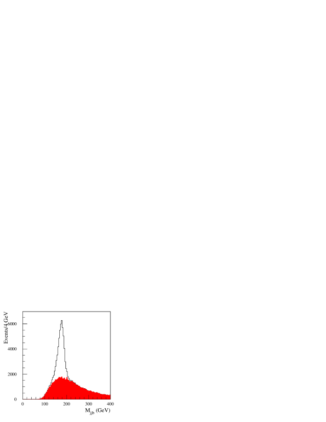
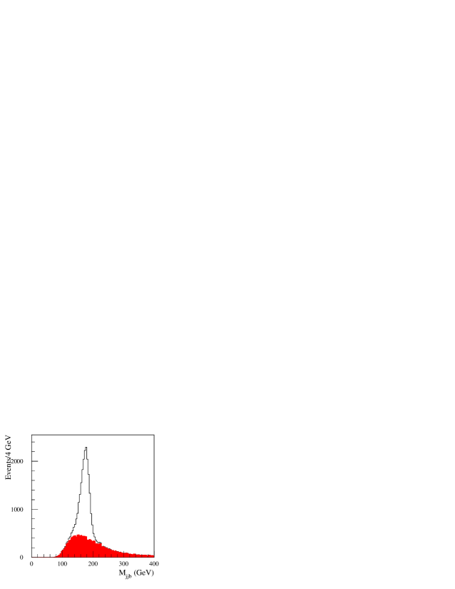
Fig. 3.: Top mass distributions for the 1 b-tagged jet sample (left plot) and the 2 b-tagged jets sample (right plot). The shaded area represents the combinatorial background. Both plots are for 10 fb^-1.

The next step is to associate a b-tagged jet to the reconstructed W. When events are selected with only one b-tagged jet, the association is performed if the b-tagged jet is closer to the reconstructed W than to the isolated lepton ($\mathchar 257\relax R(b,W)<\mathchar 257\relax R(b,lepton)$). The efficiency of this association criteria is $82\%$. In the presence of two b-tagged jets, the chosen b-tagged jet is the one giving the highest $p_{T}$ for the reconstructed top, giving an association efficiency of $81\%$. The reconstructed three jets mass distributions are presented on figure 3 for the two event selection criteria. The peak width is 12 GeV in both cases.

The overall association purity and efficiency within a top mass window of $\pm$35 GeV around the top mass peak are summarized in table 2. The top mass determination will not be limited by the statistics even if the analysis is restricted to the two b-tagged jets sample. Nevertheless, the large one b-tagged jet sample allows further dedicated cuts with negligible impact on the statistical precision of the top mass determination. In the sample with two b-tagged jets, the overall reconstruction efficiency is $1.2\%$, leading to 30000 events for one year of running at low luminosity (per 10 fb^-1). For simplicity, only this case will considered in the following.

	1 b-tagged jet sample	2 b-tagged jets sample
Top purity ($\%$)	65	69
Total efficiency ($\%$)	2.5	1.2

Table 2.: Summary table for the two samples considered. Purity and total efficiency are related to a top mass window of $\pm$35 GeV around the generated $m_{t}$ value.

2.2.2 In situ jet energy and direction calibration

As the top mass is determined from the invariant mass of a three-jet system, the accuracy of the measurement depends on how well the jet energies and directions are reconstructed. A mis-measurement of $1\%$ of the jet energies induces a top mass shift of 1.6 GeV. Similarly, a mis-measurement of $1\%$ of the cosinus of opening angle between the two jets from the W and between the reconstructed W and the b-jet induces a top mass shift of 1.2 GeV. Therefore an excellent absolute energy scale and angle measurement are required to precisely determine the top quark mass.

Numerous effects have to be taken into account to determine the initial parton energy from the energies deposited in the ATLAS calorimeters. Prior to data taking, the accumulated knowledge on the detector performances and characteristics, on physics effects like initial and final state radiations, underlying or minimum bias events plus the impact of the jet finding algorithms will allow to reach a 5-10 $\%$ on the absolute energy scale [7]. In-situ calibrations will fix the absolute energy scale through the study of known processes, taking into account in a global way the remaining inaccuracies on the knowledge on the various effects described previously.

It has been shown that an accurate absolute energy calibration of light quark jets and b-jets can be extracted from Z+jet events [7, 10], within an expected precision of about 1 $\%$. However, this calibration applied to the W mass reconstruction [11, 12], leads to a shifted W mass. Due to the energy sharing between jets, the opening angles are systematically underestimated leading to a less precise mass measurement [13].

Here, to avoid any dependency from external inputs, it is proposed to perform an situ calibration in which both the absolute energy and direction calibration are extracted from the $W\rightarrow jj$ channel itself. For this purpose, a cleaner sample of W candidates has been selected from the $t\bar{t}$ events. Initially, the jets are not calibrated but corrected for cell energy sharing effects. In addition to the preselection cuts, the di-jet invariant mass is required to fall within a mass window of $\pm$ 20 GeV around the peak value and the three-jet invariant mass to fall within a mass window of $\pm$ 15 GeV around the peak value.

The in-situ calibration is performed through a $\chi^{2}$ minimization procedure in which the dijet mass is constrained to the known W mass.

Non-calibrated jet energies are shifted from the initial parton energies due mainly to the jet cone algorithm procedure and FSR effects. However the induced shift is in general smaller than the energy resolution of the jets. This allows to fix the $\sigma_{E_{i}}$ term to the intrinsic calorimeter energy resolution. The same approach is employed for the jet directions.

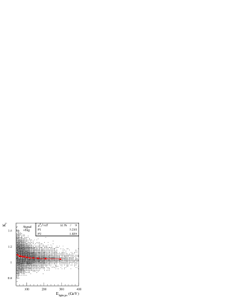
Fig. 4.: Calibration factors obtained event by event, and parametrization after calibration fit.

Fig. 5.: Final jjb invariant mass distribution.

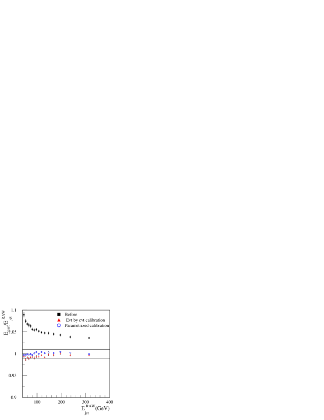
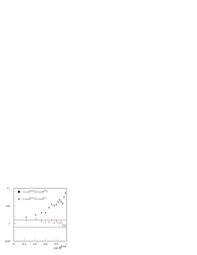
Fig. 6.: Results of the calibration fit on jet energy and direction. The two solid lines show the $\pm 1\%$ precision level.

An energy correction factor K is obtained at the end of the fitting procedure, for each jet and for each event. The distribution as a function of the raw initial jet energy is shown in figure 5. Finally, the function $\rm K=P2+\frac{P1}{E^{RAW}}$ is fitted to the distribution (the resulting parameters are shown on the figure) leading to a calibration function, without an a priori knowledge on the initial calibration function shape. In figure 6 the comparison between the initial parton energy and the calibrated jet energy at various steps of the procedure is represented. One can see the impressive effect of the in-situ calibration procedure as the ratio of the parton energy to the reconstructed jet energy remains well below the level of $1\%$. The improvement brought by this procedure is also clear on the reconstruction of the opening angle between the two jets, as seen on figure 6. It should be noted that the combinatorial background does not introduce a sizable bias on the calibration factors.

2.2.3 Top mass reconstruction

The selected three jets invariant mass distribution is shown in figure 5. The light quark jets were calibrated as described above and the b-quark jets were calibrated using Z+b events [7]. The mass peak is in agreement within 100 MeV of the generated value. The peak width is around 11 GeV, leading to a statistical error on the top mass of the order of 100 MeV for one year of running at low luminosity (per 10 fb^-1).

2.2.4 Full simulation results

The analysis presented in section 2.2 of the determination of the top quark mass using the hadronic top decay has been repeated using fully simulated events. For this purpose, 30000 $t\bar{t}$ events were processed through the GEANT-based ATLAS detector simulation package.

Events were generated under restrictive conditions at generator level. These conditions include, for example, cuts on the transverse momentum of the $t\bar{t}$ decay products. Therefore any direct comparison with the results presented in section 2.2 should be avoided. The comparison is made using the same generated events which have been passed through both the fast and full simulation package.

Fig. 7.: Top mass determination using the hadronic top decay: $m_{jj}$ and $m_{jjb}$ invariant mass distributions. The left-handed plots represent the distributions obtained from fast simulation and the right-handed plots represent the distribution obtained from full simulation.

Figure 7 represents the $m_{jj}$ and $m_{jjb}$ distributions for fast and full simulation. The $m_{jj}$ invariant mass resolution is $7.3\ \rm GeV$ for fast simulation and $8.1\ \rm GeV$ for full simulation. The $m_{jjb}$ invariant mass resolution is $11.4\ \rm GeV$ for fast simulation and $13.4\ \rm GeV$ for full simulation. In the top mass window $175\pm 35\ \rm GeV$, the signal purity and overall efficiency are $P=(79\pm 2)\%$ and $E=(6.4\pm 0.5)\%$ for fast simulation and $P=(78\pm 2)\%$ and $E=(5.7\pm 0.5)\%$ for full simulation. These results are summarized in table 3.

Quantity	Fast simulation	Full simulation
$m_{jj}$ resolution (GeV)	7.3	8.1
$m_{jjb}$ resolution (GeV)	11.4	13.4
Signal purity ($\%$) in $175\pm 35\ \rm GeV$	79	78
Signal efficiency ($\%$) in $175\pm 35\ \rm GeV$	6.4	5.7

Table 3.: Top mass determination using the hadronic top decay: comparison between fast and full simulation.

The results obtained for the signal purity and overall efficiency as well for the $m_{jj}$ and $m_{jjb}$ invariant mass resolutions are in reasonable agreement between fast and full simulation, though the resolutions from GEANT are somewhat worse. In addition, the shape and amount of the combinatorial background for both the W and top masses reconstruction are also in good agreement between the two types of simulations.

2.2.5 Systematic uncertainties

To estimate the effect of an absolute jet energy scale uncertainty, different miscalibration coefficients were applied to the reconstructed jet energy. A top mass shift per percent of miscalibration was obtained. For light quark jets, the effect is small as the jet are re-calibrated in-situ. For b-quark jets, a $1\%$ miscalibration induces a top mass shift of 0.7 GeV.

The presence of initial state radiation of incoming partons (ISR) and final state radiation from the top decay products (FSR) can impact the measurement of the top mass. To estimate their effect, a top mass shift due to ISR was computed as the difference between the value of the top mass determined with ISR switched on (usual data set) and ISR switched off. The same approach was employed for FSR. The level of knowledge of ISR and FSR is of order of $10\%$. Therefore, as more conservative estimate, the systematic uncertainty on the top mass was taken to be $20\%$ of the corresponding mass shifts.

Systematics	$\rm\delta m_{t}$ (GeV)
Light jet energy scale	0.2
b jet energy scale	0.7$\times x\%$
Initial State Radiation	0.1
Final State Radiation	$1$
b-quark fragmentation	0.1
Combinatorial background	0.1
Statistical error	0.1

Table 4.: Summary of systematic errors in the inclusive lepton plus jets sample. x represents the level at which the b jet energy scale will be known.

The b-quark fragmentation was described by the Peterson fragmentation function [14]. This function is parametrized in terms of one variable $\varepsilon_{b}$. The default value was set at $\varepsilon_{b}=-0.006$, with an uncertainty of 0.0025 [15]. The top mass was determined with another sample of events generated with $\varepsilon_{b}=-0.006+0.0025$. The difference of the top mass value between the usual sample and the latter was taken to be the systematic uncertainty on the top mass due to the knowledge of $\varepsilon_{b}$.

Uncertainties due to the combinatorial background (which is the main background) were also estimated by varying the assumptions of the background shape and size in the fitting procedure. Fits of the three-jet invariant mass distribution were performed using a Gaussian shape for the signal and either a polynomial or a threshold function for the background. The resulting systematic error on the top mass was 0.1 GeV.

All the results are summarized in table 4. The main contributions are from FSR and b-quark energy scale. Adding in quadrature all the contribution leads to a total systematic uncertainty on the top mass of the order of 1.3 GeV, provided the b-quark jets can be calibrated within $1\%$.

2.3 Top mass measurement using a kinematic fit

In the previous section, it was shown that the top quark mass can be measured in the lepton plus jets channel with an accuracy better than 2 GeV. This error is totally dominated by systematic effects, in particular the b-quark jet energy scale and FSR. In order to reduce further the systematic uncertainties, another method is proposed in the following, where the entire $t\bar{t}$ final state is reconstructed by a kinematic fit. This method is aimed to reduce the impact of poorly reconstructed jets (due to effects arising from FSR and semi-leptonic decays of b-quark jets). The final state can divided into two parts: i) the leptonic part corresponding to the leptonic top decay ($t(\bar{t})\rightarrow l\nu b(\bar{b})$) and ii) the hadronic part corresponding to the hadronic top decay ($\bar{t}(t)\rightarrow jj\bar{b}(b)$).

The hadronic part is reconstructed in a similar way to the previous section. For the light quark jets, the absolute energy scale was taken from the in-situ calibration described above and for b-quark jets, it was taken from Z+b events [7]. The invariant mass distribution of the selected di-jet pairs is reconstructed with a width on 6.2 GeV (see figure 8). The three-jet system is reconstructed with a width of 11.2 GeV (see figure 8). Over the entire mass range, the purity is $51\%$ and is increased to $71\%$ within a mass window of $\pm$ 35 GeV around the peak value.

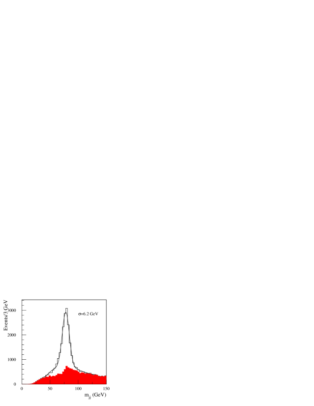
Fig. 8.: Hadronic part: reconstructed W mass (left plot) and reconstructed top mass (right plot). The combinatorial background contributions are shown (shaded areas) together with the full invariant mass distributions (full line).

Fig. 9.: Ratio of the neutrino transverse momentum at parton level over the reconstructed neutrino transverse momentum.

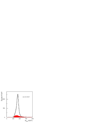
Fig. 10.: Reconstructed top mass from the leptonic part. The combinatorial background contribution is shown (shaded area) together with the full invariant mass distribution (full line).

The leptonic final state cannot be directly reconstructed due to the presence of the undetected neutrino. Nevertheless, the neutrino four-momentum can be estimated in two steps. First, the transverse component of the neutrino momentum can be approximated by the transverse missing energy (see figure 10). The longitudinal component of the neutrino momentum can then be deduced with a quadratic ambiguity, by constraining the invariant mass of the lepton-neutrino system to the known W mass value. Finally, the remaining b-tagged jet is associated to the reconstructed W. In most of the cases, there are only two b-tagged jets present in the event, and one has already been associated. In case of additional b-jets, the closest one to the isolated lepton is chosen. Per event, two leptonic top masses are computed, corresponding to the two neutrino $p_{Z}$ solutions. The distribution of the leptonic top mass the closest to the hadronic mass is represented in figure 10. It is fitted by a third order polynomial plus a Gaussian, leading to a peak width of 12.4 GeV, similar to the hadronic resolution. The event is eventually kept if one of the two leptonic top masses is within the same top mass window as the hadronic part.

Therefore, the entire $t\bar{t}$ final state can be reconstructed, with a twofold ambiguity due to the neutrino reconstruction. After selection and mass window cuts, the final sample is composed of 18000 signal events and 7000 combinatorial events (the contribution from other physical background processes is totally negligible). The total signal ($t\bar{t}$ events with all jets well assigned) efficiency is $0.7\%$ with a purity of $73\%$.

2.3.1 Top mass determination

The kinematic fit is performed in such a way that the jets and lepton energy, the jets direction (in terms of $\eta$ and $\phi$) and the three components of the reconstructed neutrino momentum can vary freely within their corresponding resolutions. The following kinematic constraints were employed:

$\rm m_{jj}=M_{W}^{PDG}$, $\rm m_{l\nu}=M_{W}^{PDG}$ and $\rm m_{jjb}=m_{l\nu b}=M_{top}^{fit}$

On an event-by-event basis and for both neutrino solutions, a $\rm\chi^{2}$ is minimized [13]. The output of the fit is the top mass estimator $\rm M_{top}^{fit}$. The neutrino solution with the lowest $\rm\chi^{2}$ is selected.

The shapes of the $\rm\chi^{2}$ distributions are different for signal and combinatorial background, as is shown in figure 11: a cut at $\rm\chi^{2}<4$ increases the $\rm t\bar{t}$ purity to more than 80$\%$. The fitted top mass is also shown in figure 11.

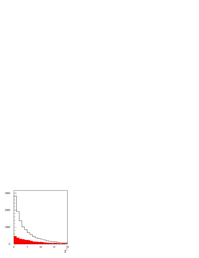
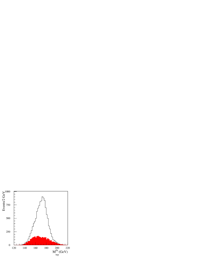
Fig. 11.: Left plot: $\chi^{2}$ distribution. Right plot: top mass after kinematic fit.

Fig. 12.: Left plot: relative difference between b-jets and b-partons energies. The shaded area defines the “badly reconstructed” b-jets. Right plot: probability to have the two b-tagged jets “well reconstructed” as a function of $\chi^{2}$.

The constraints which define the $\rm\chi^{2}$ are strong on the di-jet and the lepton-neutrino systems, due to the good knowledge of the W mass, but give a poor relative constraint on the two b-tagged jets. As a consequence, the $\rm\chi^{2}$ is directly related to the quality of the reconstruction of the b-jets, particularly as the b-jet energy can be underestimated when FSR or leptonic decays occurs. Furthermore, the quality of the top mass reconstruction can be altered, with a mass value underestimated in correlation with the effects on the b-jets energy reconstruction. The left plot of figure 12 shows the relative difference between the b-jets and b-partons energies. The jets which belong to the tail of this distribution can be defined as badly reconstructed jets. The probability to have the two b-jets “well reconstructed” decreases when the $\rm\chi^{2}$ increases (see figure 12). The top mass dependence on the $\rm\chi^{2}$ is shown in figure 15. It can be noticed that the fitted top mass becomes independent on the $\rm\chi^{2}$ if only events with “well reconstructed” b-jets are kept. To some extend, the $\rm\chi^{2}$ value allows to distinguish between “well reconstructed” b-jets from the others.

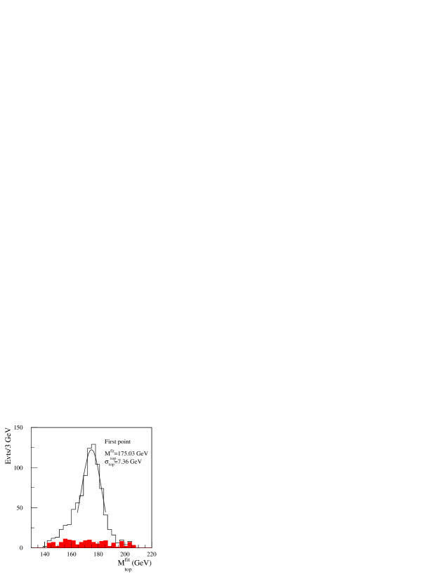
Fig. 13.: Top mass distributions for different values of $\chi^{2}$. One can observe that for the highest $\chi^{2}$ the corresponding top mass is lower, and the mass resolution is higher. The combinatorial background contributions is shown (shaded area) together with the full invariant mass distribution (full line).

The top mass is estimated in the following way. Equal samples per slices of $\rm\chi^{2}$ are built. The top mass is computed for each sample, from a Gaussian fit around $\rm\pm 1.5\sigma$ of the mass peak. Figure 13 presents two examples, for slices of $\rm\chi^{2}$ with mean values $\rm\chi^{2}=0.12\;and\;\chi^{2}=3.63$. Finally, the top mass is determined as $\rm m_{t}=M_{top}^{fit}(\chi^{2}=0)$, from a fit by a linear function to the distribution (see figure 15). In one year of running at low luminosity (per $10fb^{-1}$) the statistical error would be 120 MeV.

2.3.2 Systematic uncertainties

Fig. 14.: Fitted top mass versus $\chi^{2}$.

Fig. 15.: Reconstructed top mass versus generated top mass. The superimposed line is described by the function $M_{top}^{Rec}=P_{1}\times M_{top}^{Gen}$.

The study of the systematic uncertainties were handled in the same way as in the previous section. The results are presented in table 5. For FSR, taking $20\%$ of the mass shift obtained between FSR switched on and off leads to a systematic error on the top mass of 0.5 GeV. However, this estimate is an upper limit as the mass shift takes into account effects due to a wrong b-quark jet calibration. This effect could possibly be reduced: if the absolute b-jet scale is obtained with Z+b events generated with FSR off, the systematic error would be decreased to 0.1 GeV. This is not surprising, since when the size of the FSR contribution increases, only the slope in the figure 15 is modified. This demonstrate that events with large FSR contributions populate high $\chi^{2}$ values.

Internal Systematics	$\rm\delta m_{t}$ (GeV)
light jet energy scale	0.2
Initial State Radiation	0.1
Final State Radiation	$\leq$ 0.5
b-quark fragmentation	0.1
Combinatorial background	0.1
Total	$\leq$ 0.6
Statistical error	0.1
b jet energy scale	0.7$\times x\%$

Table 5.: Summary of the systematic errors for the top mass in the inclusive lepton plus jets sample, when the top mass is reconstructed using a kinematic fit.

The linearity of the method has been checked using several samples generated with different top masses. The same algorithm was used on all samples, with the same calibration functions for light and b jets. As is shown in figure 15 the estimated top mass depends linearly on the generated top mass.

In table 5, the errors are divided into three types: i) the statistical error, ii) internal systematic errors and iii) the systematic error due to the b-quark jet absolute energy scale which depends on external inputs. No systematic errors have been accounted for the Monte Carlo description of the decay as it has been demonstrated to be negligible [12]. Assuming the b-quark jet absolute energy scale can be determined within $1\%$, the total error on the top mass measurement is of the order of 0.9 GeV.

In summary:

$\rm m_{t}=m\pm 0.1_{\;(stat.)}\pm(0.3-0.6)_{\;(internal\;syst.)}(\pm 0.7\times x)_{\;(external\;syst.)}$

where x = b-quark jet miscalibration in $\%$.

2.4 An additional technique: mass measurement using a continuous jet algorithm

The main sources of systematic uncertainty entering in the top mass measurement in the inclusive lepton plus jets channel arise from the non-precise knowledge of the correction factors applied to the jet energy and of some physics processes parameters. In order to reduce the impact of the latter effects (mainly final state radiation) in the top mass determination, an approach based on the continuous definition of jets has been investigated [16].

This approach is based on the following ingredient: a continuous jet definition and mass estimation. This idea was first introduced in [17]. It is based on the consideration that the discrete nature of the standard jet definition may cause some problems. Two of these problems are: i) from the mathematical point of view, the breakdown of continuous distributions gives rise to instabilities (large statistical fluctuations) and therefore increases the statistical error on the measurement result, ii) the transition from a continuous energy deposition in the calorimeter to a fixed structure jet causes the loss of important information. As an example, let us consider the case of final state radiation.

As a result, the fraction of the total energy contained in the cone around the quark direction in any standard jet finding algorithm is subject to large fluctuations which cannot be precisely predicted from theory. This induces a large contribution to the systematic errors in the mass measurement. A continuous jet definition allows instead to reduce the dependence of the estimation of the details of the jet shape description in the Monte Carlo and in the jet reconstruction procedure.

In addition, this method can be coupled to a jet energy calibration based on the W mass measurement and on the reconstruction of the $t\bar{t}$ final state with a constraint kinematic fit, as presented in the previous section.

2.4.1 Method

The event selection criteria are similar to the ones used in the previously described analysis (see section 2.1). The continuous jet algorithm has been realized in the following way. Initially, a ”fixed cone” jet finding algorithm is used, with a definite cone size. For the same event, the analysis is then repeated varying the jet cone size. Here, the cone sizes range from 0.3 to 1.0 with step of 0.1.

In a preliminary stage of the analysis for each cone size a jet energy correction factor has been defined by calculating the two-jet invariant mass distribution for non b-tagged jets with $p_{T}>40$ GeV. The W-peak position has been fitted using the sum of a Gaussian and Tchebyshev polynomials up to the fourth order.

The same corrections as for the light quark jets have been applied for the b-jets, even if not being the optimal ones. Two non b-tagged jets with $p_{T}>40$ GeV have been selected for which the combined invariant mass was close to the mass of the W peak for a given cone size chosen for the jet reconstruction algorithm. The requirement $|M-M_{W_{true}}|<25~{}~{}GeV$ has been used. A b-quark jet energy rescaling has been applied to the b-tagged jets with $p_{T}>40$ GeV, according to the correction factor for the given cone size. At least two b-quarks are required in each event. If there are more, the combination with the highest $p_{T}$ is selected.

For the given cone size, a constraint fit procedure was then applied to the selected jets. This kinematic fit uses three constraints $m_{jj}=M_{W}$, $m_{l\nu}=M_{W}$ and $m_{l\nu b}=m_{jjb}$ which, together with the missing momentum measurement, allows to determine the neutrino momentum unambiguously. Only the energies of the jets are tuned during the fit. However, in the method proposed here, a slightly different approach has been exploited to improve the accuracy of the reconstruction procedure: a robust modification [18, 19] of the fitting functional have been used instead of the usual $\chi^{2}$ [16].

Only the events with a small minimum value of the fitting functional have been retained. This value is not a $\chi^{2}$ because of the robust fitting method and depends on jet and missing momentum error parameterizations. The invariant mass of the 3-jet system obtained after the constraint fit has then been considered as the top quark mass estimate for the current event and current jet cone size.

After having a top quark mass estimate for a certain jet cone size, the cone size is changed and the whole procedure is repeated for the given event, starting again from the jets finding. If the jet finding procedure is unable to find the required minimum number of jets with $p_{T}>40$ GeV the algorithm skips to the next event. All the top quark masses calculated for all the events and all the jet cone sizes are finally summed up in one single histogram. The distribution obtained as the result of the reconstruction procedure is shown in the left plot of figure 16.

For different events, the mass value at the peak position is obtained for different cone sizes. The point here is that a position of accumulation should be a more robust estimator of the jet system invariant mass with respect to the single value which is obtained by calculation of only one mass for each event. In figure 17 the 3-jet system invariant masses (the top quark mass estimator) are shown as a function of the cone size $\mathchar 257\relax R$ as well. The summed distribution for all the $\mathchar 257\relax R$ values is shown at the bottom of figure 17.

Fig. 16.: Left plot: Summary distributions of the top quark mass estimates for all cone sizes. Right plot: Difference between the generated and reconstructed top quark masses, for different top mass values, after having applied the mass reconstruction procedure as described in the text. The result of a linear (constant) fit is also shown.

Fig. 17.: Mass distributions for the three jets system and for various cone sizes. The vertical line indicates the generated top mass value. The bottom-right plot represents the sum of all distributions.

The top quark decay peak is then fitted with a Breit-Wigner function including a 4th order Tchebyshev polynomial to describe the background. The position of the peak is considered as the final estimate of the top quark mass. The Breit-Wigner shape has been selected because it gives a much better description of the signal compared with a Gaussian shape. However, an equally good $\chi^{2}$ may be obtained by using a sum of two Gaussian with the same mean for the signal description. The difference between the results with the two methods has been treated as a systematic error.

2.4.2 Results

A typical mass distribution obtained by applying the top quark mass reconstruction procedure described above is shown in figure 18 for 400000 $t\bar{t}$ generated events with $m_{t}^{MC}=175$ GeV.

A mean statistical error of the top quark mass estimation obtained with the fit of the mass distribution in figure 18 by a Gaussian function plus a 4th order polynomial background is $\delta m_{t}\sim 100$ MeV, for 400000 generated events.

In order to evaluate the statistical properties of the top quark mass estimation procedure from $\delta m_{t}$, some additional steps are needed. Due to the continuous jet definition method and to the data based b-jet energy correction, the statistical error given by the fit of the distribution is not correct. The invariant mass distributions obtained from the same event sample with different cone sizes used by the algorithm are strongly correlated and cannot be treated as independent. The statistical error of the b-jet energy correction factors has to be taken into account. Both effects lead to an underestimate of the statistical error as obtained from the invariant mass distribution fitting procedure. For the correction, one should rescale statistical errors from the fitting procedure. On the other side the mass distributions obtained with the different jet cone sizes are not the same because even the number of reconstructed jets in event may be different for $\mathchar 257\relax R=0.3$ and $\mathchar 257\relax R=1.0$, then the summed distribution has more information than one obtained with the single $\mathchar 257\relax R$. So one must rescale a statistical error obtained in the fitting procedure by a factor in the range $1...\sqrt{8}$. The determination of such rescaling factor is not an easy task to be performed analytically. However, one can easily determine the corresponding correction in Monte Carlo experiment, with the help of pull distribution. For each of the top quark masses ($m_{t}=165,170,175,180,185$ GeV), $400000$ events were generated and reconstructed. This procedure has been repeated five times. The differences between the generated and reconstructed top masses are determined for all input top masses and the corresponding pull distribution is obtained. The dispersion of the pull distribution (equal to the scaling factor) is 1.6. After multiplying $\delta m_{t}$ by 1.6, taking into account b-tagging efficiency and rescaling to an integrated luminosity of 10 fb^-1, an estimated statistical error about $\delta m_{t}\sim 65$ MeV is found. The final statistical error of the top mass will be less than 100 MeV.

2.4.3 Systematic errors

As expected, and as can be seen in figure 17, the reconstructed three-jet mass depends on the jet cone size. The final value extracted for the top mass will, therefore, depend on the choices for the minimum and maximum cone sizes to use in the analysis. The analysis, which used a cone size step of 0.1 with minimum and maximum values of 0.3 and 1.0 respectively, was re-done excluding either the minimum or maximum values and again by shifting the grid of cone sizes by 0.05. The largest change observed in the resultant top mass, namely 250 MeV, has been assigned as the systematic error in the top mass due to uncertainty in the range of cone sizes to use.

The effect of the $\chi^{2}$ cut value on the determination of the top mass has been checked. The difference between the reconstructed top mass and the generated value has been plotted versus the $\chi^{2}$ cut value. A maximum difference of 200 MeV was found. This value has been taken as the systematic error due to the $\chi^{2}$ dependence of the top quark mass determination.

The description of the background and signal shapes in the fitted invariant mass distribution has been taken into account. Changing the background description, the degree of polynomial, the top mass peak shape from a Gaussian to a Breit-Wigner or to the sum of two Gaussians with common means lead to a systematic error on the top mass of 90 MeV.

The effects of initial and final state radiation have been computed in the same way as before. The systematic error due to ISR is found to be negligible and the error due to FSR is found to be 200 MeV.

Fig. 18.: Reconstructed top mass. The full fine represents the result of a fit by a Gaussian plus a 4th order polynomial.

Since the light quark jets are calibrated in-situ, a negligible systematic error in the top mass measurement results from the uncertainty in the light quark jet energy scale. For the b-jet energy scale, a 1% miscalibration induces a top mass shift of 700 MeV, as was discussed in section 2.3.2 for the kinematic fit with fixed cone size.

A study was performed to investigate whether one could reduce the b-jet energy scale systematic error by calibrating the b-jets using the same in-situ calibration obtained for the light quark jets. Proceeding this way will increase the statistical error, due to the data based calibration, but also introduce a systematic shift of the top mass due to any differences of energy losses between light quark jets and b-jets. These differences are expected due to physics effects, and also due to detector and reconstruction effects. The systematic error due to the b-quark fragmentation parameter $\epsilon_{b}$ was estimated as before and was found to be 50 MeV. The b-jet energy scale depends also on the branching fraction of the semi-leptonic b-hadron decays, due to the presence of the undetected neutrino. To estimate the influence of the imprecise knowledge of the semi-leptonic decay fraction of b-hadrons (which is known with an accuracy of $7\%$), all semi-leptonic branching ratios were scaled by 1.07 in the Monte Carlo, resulting in a top mass shift of 60 MeV. Due to the fixed jet cone reconstruction procedure, the b-jet energy scale depends on the parton shower evolution and in particular on the $\alpha_{s}$ evolution parameters. Introducing the b-quark mass corrections into the default $\alpha_{s}(p_{T})$ evolutions in showers led to a systematic error of 90 MeV. Combining these uncertainties in quadrature would give a total systematic error on the top mass due to the differences of the physics effects between light quark jets and b-jets of 130 MeV. While this result is very encouraging, it must be stressed that these comparisons were made using a fast, parameterized Monte Carlo description of the ATLAS detector. Further study will be performed with full GEANT-based simulation of the detector to increase the confidence of this potential reduction in the systematic error.

The shape of the W signal used to rescale the b-jet energy is another source of systematic uncertainty. The systematic error was estimated by taking into account the asymmetric shape of the W signal distribution, changing the background shape under the W peak and the fitting region. These sources account for a systematic error on the top mass of 100 MeV.

The various contributions to the top mass systematic error for the continuous jet analysis are summarized in table 6. Adding the various contributions in quadrature leads to a total systematic error on the top quark mass of the order of 1 GeV, dominated by the uncertainty in the external calibration for the b-jets. Should it be possible to realize the improvement suggested by the study of b-jet calibration using the in-situ light quark calibration, the total error could be reduced to of order 400 MeV.

Source	$\rm\delta m_{t}$ (GeV)
Range of jet cone sizes	0.25
$\chi^{2}$ dependence	0.2
Signal and background shape	0.1
ISR and FSR	0.2
External b-jet calibration 1%	0.7
Internal b-jet calibration
Physics effects	0.13
W signal shape	0.1

Table 6.: Summary of the systematic errors for the top mass in the inclusive lepton plus jets sample, when the top mass is reconstructed using a continuous jet definition. For more details, see the text.

2.5 Summary

Three methods to determine the top quark mass in the lepton plus jets channel have been presented in chapters 2.2, 2.3 and 2.4. In the first method (2.2) the top mass is extracted from the invariant three jets mass of the hadronic top decay, in the second method (2.3) the top mass is determined from a kinematical fit of the entire $t\bar{t}$ decay, and in the third method the top mass is determined from a kinematic fit and using a continuous jet algorithm. The main sources of uncertainties arise from final state radiation and b-quark jet energy scale. It was shown that the contribution from light quark jets energy scale to the systematics errors can be reduced to a negligible level using an in situ calibration. Provided that the b-quark jet absolute energy scale can determined within $1\%$, the top quark mass can be measured with a precision at the level of 1 GeV in one year of LHC running at low luminosity (per $10fb^{-1}$).

2.6 Top mass measurement using large $p_{T}$ events

In this section, we present an alternative method which uses a special sub-sample of the single lepton plus jet events where the top has high transverse momentum, for example $p_{T}>200$ GeV.

In this topology, the two quarks are produced back-to-back, and the daughters from the two top decays would appear in distinct hemispheres of the detector: the “hadronic” one from the decay $t\rightarrow Wb\rightarrow jjb$, and the “leptonic” one from the decay $t\rightarrow Wb\rightarrow l\nu b$. Due to the high $p_{T}$ of the event, detector systematics as well as backgrounds from other processes are expected to be very small. The distinct feature of these events which is exploited here, is the fact that due to the high $p_{T}$ the three jets from the hadronic top decay tend to overlap in space, as shown in figures 20,20, and 22.

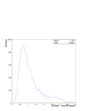
Fig. 19.: $\mathchar 257\relax R$ distance between the top quark and the furthest quark from the hadronic W decay.

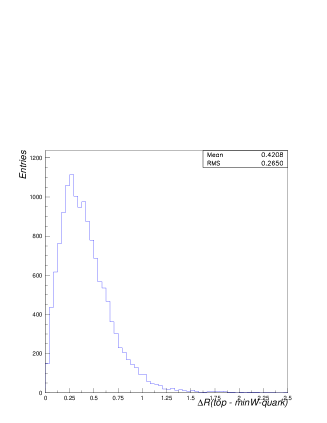
Fig. 20.: $\mathchar 257\relax R$ distance between the top quark and the closest quark from the hadronic W decay.

Therefore one could reconstruct the top mass without using the jets as in the methods described in the previous section, but from summing up the individual calorimeter towers over a large cone ($\mathchar 257\relax R$ in [0.8-1.8]) around the top direction. The top direction itself can be determined in two ways: i) as opposite to the top direction reconstructed in the leptonic decay, where the missing energy in the event is used to reconstruct the neutrino, and ii) as the direction of the invariant mass of the three jets in the hadronic top decay. Figure 22 shows the percentage of the generated events with all the three jets from the hadronic top decay lying within a distance $\mathchar 257\relax R$ from the top quark direction.

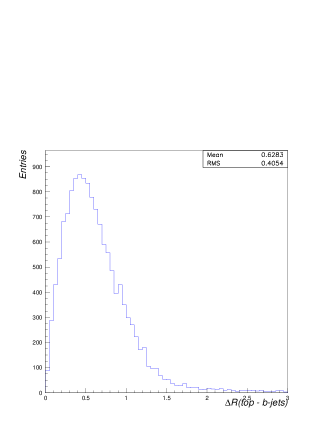
Fig. 21.: $\mathchar 257\relax R$ distance between the top and the b-quark at parton level.

Fig. 22.: Percentage of the events having all the three jets from the hadronic top decay within a cone aperture $\mathchar 257\relax R$ from the top, at parton level.

Using directly the calorimeter towers, avoids problems with the jet reconstruction and energy calibration, one of the major source of systematic errors in the top mass measurement, and introduces a different set of systematic errors. This method is therefore very interesting and useful for the final combined top mass determination by ATLAS.

2.6.1 Event selection and reconstruction

Samples of high $p_{T}$ $t\bar{t}$ events were generated with a cut of 200 GeV in the center of mass of the hard scattering. The cross-section of this topology corresponds to about $2\%$ of the total $t\bar{t}$ cross-section. Events are selected to pass the trigger selection and by requiring one isolated lepton with $p_{T}>30$ GeV and $|\eta|<2.5$, the transverse missing energy greater than 30 GeV ($E_{T}^{miss}>30$ GeV), and at least four jets reconstructed using a cone of $\mathchar 257\relax R$ = 0.4 with $p_{T}>40$ GeV and $|\eta|<2.5$, of which two must be tagged as b-jets.

The overall efficiency is 9$\%$, resulting to $\sim$15000 selected events per (10 fb^-1) . Due to the high $p_{T}$ of the event and the requirement for two tagged b-jets, the background (mainly W+jet, WW or QCD events) is reduced into negligible levels and therefore not discussed further.

For the events passing the preselection cuts described above, the top quark direction was determined as described. First the hadronic W invariant mass was reconstructed from the two highest $p_{T}$ non b-tagged jets. Combinations where $m_{jj}=M_{W}\pm 20$ GeV were selected. The two jets were combined with the closest b-jet to reconstruct the top. Finally, the reconstructed top $p_{T}$ was required to be above 235 GeV. After all the cuts $\sim$3600 events remain per $10^{-1}$ fb, with an overall efficiency of $2\%$.

Once the top direction is determined, the invariant mass of all the calorimeter towers ($\mathchar 257\relax\eta\times\mathchar 257\relax\phi=0.1\times 0.1$) around this direction is evaluated according to the formula:

$$m_{clust}^{2}(\mathchar 257\relax R)=(E^{2}-p^{2})=(\sum_{i=1}^{n(\mathchar 257\relax R)}E_{i})^{2}-(\sum_{i=1}^{n(\mathchar 257\relax R)}\mathchoice{\mbox{\boldmath$\displaystyle\bf p$}}{\mbox{\boldmath$\textstyle\bf p$}}{\mbox{\boldmath$\scriptstyle\bf p$}}{\mbox{\boldmath$\scriptscriptstyle\bf p$}}_{i})^{2}.$$

where $E_{i}$ is the total calorimeter energy in the i-th tower evaluated in electromagnetic scale, and $\mathchoice{\mbox{\boldmath$\displaystyle\bf p$}}{\mbox{\boldmath$\textstyle\bf p$}}{\mbox{\boldmath$\scriptstyle\bf p$}}{\mbox{\boldmath$\scriptscriptstyle\bf p$}}_{i}$ is its three momentum vector. The index $n(\mathchar 257\relax R)$ runs over all the towers within the selected cone radius. This invariant mass is directly proportional to the top quark mass: $m_{clust}=m_{clust}^{top}$.

Figure 24 shows the reconstructed $m_{clust}^{top}$ invariant mass for a cone size of $\mathchar 257\relax R$=1.3. A clear Gaussian distribution is observed with the peak value around the nominal top mass. Fitting the peak region with a Gaussian, we obtain a peak width of 9.6 GeV, comparable to that obtained with the jet method.

Fig. 23.: Reconstructed $m_{clust}^{top}$ spectrum for $\mathchar 257\relax R$=1.3.

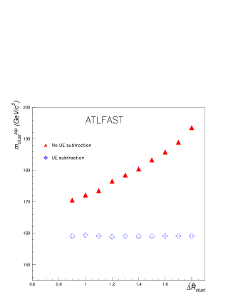
Fig. 24.: Fitted $m_{clust}^{top}$ invariant mass, as a function of the cone size, before and after the $UE_{tower}$ is subtracted.

As shown in figure 22, more than 80$\%$ of the events where the three jets are at $\mathchar 257\relax R\leq 1.3$ from the top quark direction are selected.

The invariant mass $m_{clust}^{top}$, is evaluated using various cone sizes in the range from $\mathchar 257\relax R$=0.8 to 1.8, as there is no reason a priori to select a given value. On the contrary, the resulting invariant mass has to be independent from the cone size used. For each $\mathchar 257\relax R$ cone size, a Gaussian is fitted around the peak position in the invariant mass $m_{clust}^{top}$ distribution. The fitted peak values for the different cone sizes are shown in figure 24. The variation observed can be attributed to the Underlying Event contribution which is added for each calorimeter tower, resulting in an increased invariant mass value as the cone size increases. A method to evaluate the UE contribution in each tower follows.

2.6.2 The Underlying Event (UE) estimation

The Underlying Event contribution per calorimeter tower ($UE_{tower}$) was estimated from the same high $p_{T}$ top sample. It represents the average transverse energy $E_{T}$ deposited per calorimeter tower in each event, once all the towers related with the high $p_{T}$ products are excluded. The values as well as the number of towers used in each case have been computed for different rapidity regions [22]. An average over all rapidity and isolation cut range, gives a value of $UE_{tower}$=447.5 MeV, which is subtracted from the energy of each tower in the calculation of $m_{clust}$.

In figure 24 the invariant mass $m_{clust}^{top}$ is shown after the the $UE_{tower}$ is subtracted. The resulting values are now independent of the cone size, with an average value of 159 GeV and with all values within $\pm$0.15$\%$. Varying the $UE_{tower}$ by $\pm$10$\%$, a cone size dependence is again observed, raising to a bit less than $\pm$2$\%$, which demonstrates that the value used is the correct one and gives the precision required for the target top mass measurement error. In ATLAS, once the real data become available, the $UE_{tower}$ will be calculated in situ as done here, but also using other event samples, resulting to an overall error of about $10\%$.

2.6.3 Mass scale calibration

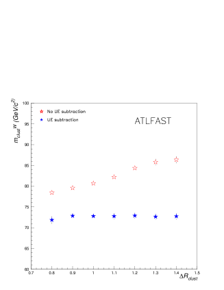
Fig. 25.: The fitted $m_{clust}^{W}$ invariant mass, before and after UE subtraction.

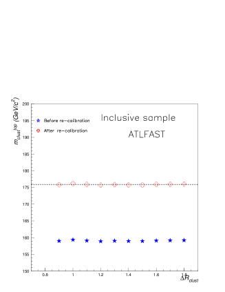
Fig. 26.: The fitted $m_{clust}^{top}$ invariant mass, after $UE_{tower}$ subtraction and after mass scale is applied.

After the $UE_{tower}$ contribution is subtracted, the reconstructed $m_{clust}^{top}$ invariant mass has become independent of the cone size, but the resulting values are now $\sim$9$\%$ lower than the generated top quark mass. This a priori is expected as no particular mass scale or absolute energy scale has been used so far. As a first attempt the $m_{clust}^{top}$ values could be calibrated using the Monte Carlo data. However doing so the method will be dependent on the exact modelling of the process and won’t be anymore a “direct” measurement of the top mass. The best way is to obtain a mass scale calibration using the data themselves.

The method studied here is to apply the same reconstruction procedure, with the same $UE_{tower}$, to other known particles with well measured masses and extract from there the necessary mass scale calibration factors. In our case the easiest way is to use the inclusive top sample and apply the same reconstruction method to the W mass reconstruction. This sample offers high statistics, and has practically the same event topology as the high $p_{T}$ sample. Rescaling the corresponding $m_{clust}^{W}$ invariant mass values to the nominal mass of the W, we can obtain the mass scale calibration coefficient $C_{top}$ averaging all the cone sizes $\mathchar 257\relax R$. Finally, to determine the top mass, the average value of all the $m_{clust}^{top}$ values after calibration is used. Fixing the mass scale with the W, and then transferring the results to the top, it implies that the same calibration is used for the both the light quarks and the b-jets.

Events were generated in the single lepton plus jets topology, without $p_{T}$ cut applied to the hard scattering process. The large statistics available, allow to apply tight cuts in order to select events where the two jets from the hadronic W decay are close in space (as in the high $p_{T}$ sample) and at the same time far away from the b-jet. Events were selected by requiring an isolated lepton with $p_{T}>20$ GeV and $|\eta|<$2.5, $E_{T}^{miss}>20$ GeV, at least four jets (reconstructed in a cone of $\mathchar 257\relax R$=0.4), with $p_{T}>40$ GeV and $|\eta|<$2.5, of which two are tagged as b-jets. In addition, the distance between the two highest non b-tagged jets, should be $\mathchar 257\relax R<$1.3 and the two b-jets of the event should be at a distance $\mathchar 257\relax R\geq$2.0 away from the reconstructed W direction.

The two highest $p_{T}$ non b-tagged jets were used to reconstruct the W and find its direction. Then the $m_{clust}^{W}$ invariant mass was calculated around this direction subtracting from each tower the same $UE_{tower}$ as calculated before. In figure 26 the fitted value of the invariant mass $m_{clust}^{W}$ are shown. As for the top, the reconstructed values after the UE is subtracted become independent from the cone size (within $\pm$0.7$\%$) and about 7.7 GeV lower than the nominal W mass.

Figure 26 shows the resulting $m_{clust}^{top}$ values after the mass scale calibration is applied. The variation between the points is $\pm$0.22%. As an example, for $\mathchar 257\relax R$=1.2(1.3) the $m_{clust}^{top}$ invariant mass after the $UE_{tower}$ subtraction was 158.9(159.0) GeV, and after applying the calibration becomes 175.7(175.8) GeV. Taking the average of the calibrated $m_{clust}^{top}$ invariant mass for all cone sizes, a value for $m_{t}=175.9$ GeV is obtained, which is within 0.5$\%$ from the generated top quark mass.

Fig. 27.: Reconstructed $m_{clust}^{top}$ spectrum obtained using a cone size of $\mathchar 257\relax R$=1.3 around the top direction.

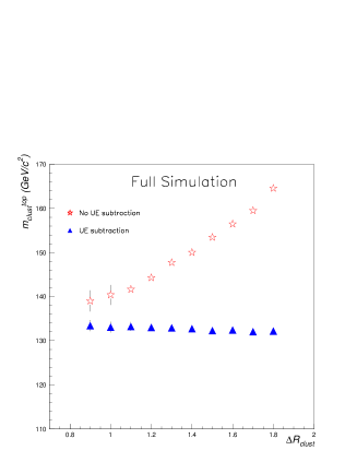
Fig. 28.: The $m_{clust}^{top}$ invariant mass dependence on the cone size before and after the $UE_{tower}$ is subtracted.

2.6.4 Full simulation results

The results presented so far were obtained using the fast detector simulation [9]. The same analysis was repeated with a sample of full (GEANT-based) simulated events of the ATLAS detector. Figure 28 shows the reconstructed $m_{clust}^{top}$ invariant mass spectrum for a cone size of $\mathchar 257\relax R$=1.3. The variation of the fitted values for different cone sizes is shown in figure 28.

Although the peak values in this case are lower than those of the fast simulation, the overall variation for the same cone size range stays about the same. The difference between the fast and full simulation can be attributed to the shower shape development which is not included in the fast simulation.

The $UE_{tower}$ was evaluated following the same procedure as before. The average $UE_{tower}$ is now 42.5 MeV [22], much lower than the fast simulation. Since now there are more calorimeter towers contributing but with lower energy in each, compared to the fast simulation case where the energy for each particle is deposited to a single tower. This value was used for all the full simulation studies described below.

The $m_{clust}^{top}$ invariant mass after the $UE_{tower}$ subtraction is shown in figure 28 as a function of cone size used. As expected, it remains basically independent from the cone size, but lower by $24.6\%$ from the generated top mass. The variation observed, $\pm$0.9$\%$, is bigger than with the fast simulation sample, and can be attributed to the poor quality of the fits due to the lack of statistics. Using only the points up to $\mathchar 257\relax R$=1.4 the average value is 133 GeV, with a variation of $\pm$0.2$\%$.

The same mass scale calibration procedure was used, with a sample of 30000 fully simulated inclusive $t\bar{t}$ events, applying the same cuts and reconstruction procedure. The fitted $m_{clust}^{W}$ peak values for different values of $\mathchar 257\relax R$ are shown in figure 30, before and after the $UE_{tower}$ is subtracted.

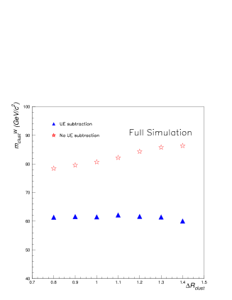
Fig. 29.: The fitted $m_{clust}^{W}$ invariant mass, before and after the $UE_{tower}$ is subtracted.

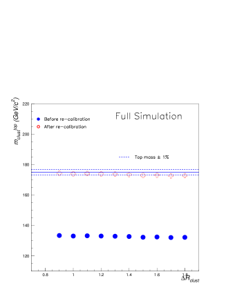
Fig. 30.: The fitted $m_{clust}$ invariant mass before and after rescaling and $UE_{tower}$ subtraction and as a function of the cone size.

After the UE contribution is subtracted, the resulting $m_{clust}^{W}$ invariant mass remains independent from the cone size but 23.5$\%$ below the nominal W mass. The mass scale is determined as before, and $m_{clust}^{top}$ invariant mass values after the calibration factors are applied are shown in figure 30. The resulting values are constant within $\pm 1.4\%$ from the generated top quark mass, for the whole range of cone values used. The average $m_{t}$ is 172.6 GeV, which is 1.4$\%$ below the generated top mass, and with all points within $\pm$0.9$\%$. Restricting to the range up to $\mathchar 257\relax R\leq$1.4, where basically we run out of statistics, the $m_{t}$ changes to 173.8 GeV, with the points now having a spread of $\pm$0.3$\%$.

In summary, the full and fast simulation data show the similar results and confirm the competitiveness of the proposed reconstruction method. However, further studies with larger statistics samples should be made in particular for high $\mathchar 257\relax R$ values.

2.6.5 Systematic uncertainties

Several studies have been performed which cover most of the possible systematic errors. Studies requiring large statistics and several settings of generator parameters were performed with the fast detector simulation, while for the cases where the exact detector response is important samples of full detector simulation were used. In some cases where large computing effort was required only the sensitivity of the results was investigated without going to details. More information on these studies can be found in [22].

To study the linearity of the reconstructed top mass several samples of high $p_{T}$ top events with different input top quark mass in the generator from 160 GeV to 190 GeV were produced and analyzed in exactly the same way. For all the samples, the same $UE_{tower}$ and mass scale calibration factors obtained as explained before were used. In the mass range 170-180 GeV, the reconstructed top mass is in very good agreement with the generated value. For larger values a bigger error is observed which is somehow expected as the event environment changes and the UE and mass scale calibrations are not optimal anymore.

The sensitivity to initial (ISR) and final (FSR) state radiation was studied in the same way as in other analysis. Samples of high $p_{T}$ top events were generated with the ISR or FSR contributions switched off at the generator level, and the analysis was repeated keeping the same $UE_{tower}$ estimate and the mass scale calibration factors. Doing so, and for a cone radius $\mathchar 257\relax R=1.3$ a shift in the reconstructed top mass of 0.7(0.3) GeV is observed when ISR(FSR) was not present. It has to be pointed out this error is a very pessimistic approach, as the exact level of the ISR(FSR) contributions in the events will be measured and known at LHC to about 10% level and the generators will be correctly tuned to this. Therefore as in the other analysis, the final error quoted for the top mass is 20% of the total mass shift observed, equal to 0.1 GeV.

The sensitivity on the b-quark fragmentation was studied by generating samples where the $\epsilon_{b}$ parameter in the Peterson formula was varied within its error currently at 0.0025 [14]. The top mass was reconstructed in each sample using the same $UE_{tower}$ and mass scale. The observed top mass shift among the samples is quoted as the error due to this effect. As an example, for a cone size of $\mathchar 257\relax R$=1.3 the mass shift was 0.3 GeV. Similar values obtained for other cone sizes.

The UE energy estimate per tower plays an important role in this top reconstruction method. To evaluate the sensitivity of the reconstructed mass due to this, the value calculated (447.5 MeV for the fast and 42.5 MeV for the full simulation data) was varied by $\pm$10% and the top reconstruction and the mass scale calibration was repeated each time. As shown in figure 32 the reconstructed values stay well within $\pm 1\%$ of the generated value.

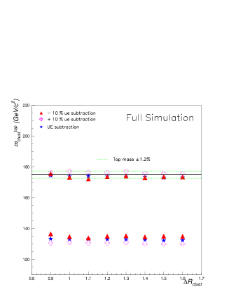
Fig. 31.: Reconstructed $m_{clust}^{top}$ mass dependence on the $UE_{tower}$ energy estimate. At each case the mass scaling factors have been recalculated as explained in the text.

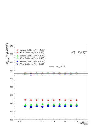
Fig. 32.: Reconstructed $m_{clust}^{top}$ mass values before and after the rescaling from the W reconstruction in the inclusive sample for three values of $e/h$.

To study the contribution of a possible calorimeter mis-calibration in the top mass measurement, the energy in each tower was varied according to a Gaussian with different values of sigma from 1 to 5%, well beyond the expected reach by ATLAS. The analysis was repeated in each case keeping the $UE_{tower}$ unchanged. For a cone size of $\mathchar 257\relax R=1.3$ the observed shift in the reconstructed top mass is 0.6(1.2) GeV when a mis-calibration of 1(5)% is added (0.7(1.3) GeV in full simulation). This value however is rather pessimistic, since whatever the cell mis-calibration would be the $UE_{tower}$ would be computed accordingly, and the whole error will be incorporated into the mass scale calibration.

Tests with the ATLAS calorimeter prototypes have shown that the combined $e/h$ is different than 1.0 [23]. Moreover it was demonstrated that in both fast and full detector simulation programs the $e/h$ effect on the calorimeters is not correctly treated [24]. To study the sensitivity of the reconstructed top mass due to this, given that in this method the individual calorimeter towers that combine information from several calorimeters is used, several fast simulation samples were generated where the energy deposited by hadrons has been corrected according to the Groom’s formula [25] thus simulating values of $e/h$ between 1.0 and 1.63. The whole analysis was repeated in each case. Changing $e/h$ to 1.63, a rather extreme value, the $UE_{tower}$ estimate changes from 447.5 MeV to 417.5 MeV, and the reconstructed top mass by 0.7%, as expected from the mass scale calibration procedure.

Since for the top mass reconstruction the whole calorimeter volume is used, either to calculate the UE contribution either to evaluate the top mass, the presence of electronics noise may have an impact on the results. To study this, a test using the full simulated data was performed, where the electronics noise was added as Gaussian noise to the cell energies according to the expected values for each calorimeter. Repeating the same procedure as before, the $UE_{tower}$ value changes from 42.5 MeV to 16 MeV, a surprising low value. Following the same procedure and applying the mass scale calibration, the average reconstructed top mass, is 175.17 GeV but shows a variation within $\pm$ 1.2% for the full range of cone sizes used between 0.9 and 1.6, partially enhanced due to the lack of statistics. Further studies are needed to fully understand the effect, once the detector is built.

2.6.6 Summary

The method presented here uses a special sub-sample of the single lepton plus jet events where the top has high transverse momentum. The case with $p_{T}>200$ GeV was studied here, which due to the high $t\bar{t}$ production at LHC offers good statistics per year at low luminosity ($10fb^{-1}$).

After some pre-selection cuts aiming to efficiently select the hadronic top decay products with minimal contribution from the background, the top direction is found using jets similarly to the inclusive sample. Then, using the unique feature of these events, where the hadronic top decay products are well collimated in space, all the calorimeter towers within a cone of radius $\mathchar 257\relax R_{clust}$ around the reconstructed top direction are summed, forming a top invariant mass. It was then shown that the reconstructed invariant mass becomes independent of the cone radius used (varied between 0.8 and 1.8) once the underlying event contribution is subtracted. Finally, the mass scale was determined by applying the same reconstruction method for the $W\rightarrow jj$ decay in the top events of the inclusive sample. After recalibration, the results obtained with both the fast and full detector simulation are comparable with the other methods, and demonstrate that the top mass can be reconstructed with an accuracy of 1%.

Using this method the reconstructed top mass is sensitive to a different set of systematic errors, a first study of which as was performed. From the results obtained, the major contribution is in the mass scale calibration procedure, with all the errors stay below the 1$\%$ level. Table 7 summarizes results. For some of the studies described above, the final systematic error once the detector and the data are available will be incorporated in the mass scale calibration procedure, therefore are not included as individual lines in the table.

	$|\mathchar 257\relax m_{t}|$ (GeV)	$\delta m_{t}$ (GeV)
Initial state radiation	0.7	0.1
Final state radiation	0.3	0.1
b-quark fragmentation	0.3	0.3
UE estimate ($\pm 10\%$)	1.3	1.3
mass scale calibration	0.9	0.9

Table 7.: Top mass shift ($|\mathchar 257\relax m_{t}|$) and quoted systematic error on $m_{t}$ ($\delta m_{t}$) due to various sources of systematic uncertainties.

3 Top mass measurement in the dilepton channel

The dilepton events can provide an indirect measurement of the top quark mass. The difficulty comes from the fact that, in principle, one cannot fully reconstruct the top decays due to the presence of undetected neutrinos in the final state. For the determination of the top mass, previous methods have exploited the correlation between the top mass and kinematic quantities, such as the mass $m_{lb}$ of the lepton-b-jet system [7].

Here, in a first step, assuming a value for the top mass, it is proposed to reconstruct the top decays by solving the set of equations describing the kinematic constraints of the decays. Then, to determine the top mass, the solutions obtained for different input top masses will be compared to the data [26].

3.1 Event selection

The dilepton events are characterized by two high $p_{T}$ isolated leptons, large traverse missing energy $E_{T}^{miss}$ and two jets coming from the fragmentation of the b-quarks. Taking into account the branching ratio, about 400000 dilepton events can be expected for integrated luminosity $10fb^{-1}$.

The background is coming mainly from Drell-Yan processes and $Z\rightarrow\tau\tau$ associated with jets, and from WW+jets and $b\bar{b}$ production. Events are selected by requiring two opposite sign isolated leptons with $p_{T}>35$ GeV and $p_{T}>25$ GeV respectively and $|\eta|<2.5$, $E_{T}^{miss}>40$ GeV, and two jets with $p_{T}>25$ GeV. After event selection, 80000 signal events are left, with a signal over background ratio around 10.

3.2 Method for the final state reconstruction

For the determination of the momenta of both the neutrino ($\nu$) and anti-neutrino ($\bar{\nu}$), it is assumed that the masses of the top and anti-top are known. The reconstruction algorithm is based on solving a set of equations coming from the kinematic properties of the conservation of momentum and energy [26]. The set of equations consists of six equations for six unknown components of momenta of neutrino and antineutrino. First two equations describe conservation of transversal momentum of the $t\overline{t}$ system, assuming that this momentum is 0. The other equations constrain invariant masses of both lepton+neutrino systems to the masses of $W^{+}$ and $W^{-}$ bosons, and masses of both lepton+neutrino+jet system to the masses of top and antitop quarks. All $W^{+}$, $W^{-}$, top and antitop masses are assumed to be known.

After some derivations [26], the following two linear equations with the unknowns $p_{x}^{\overline{\nu}}$, $p_{y}^{\overline{\nu}}$, $p_{z}^{\overline{\nu}}$ and $p_{z}^{\nu}$, are obtained:

$$\left(2\frac{{E_{\overline{b}}p_{x}^{l^{-}}}}{{E_{\overline{l}}}}-2p_{x}^{\overline{b}}\right)p_{x}^{\overline{\nu}}+\left(2\frac{{E_{\overline{b}}p_{y}^{l^{-}}}}{{E_{\overline{l}}}}-2p_{y}^{\overline{b}}\right)p_{y}^{\overline{\nu}}+\left(2\frac{{E_{\overline{b}}p_{z}^{l^{-}}}}{{E_{\overline{l}}}}-2p_{z}^{\overline{b}}\right)p_{z}^{\overline{\nu}}$$ (1)

$$+2E_{\overline{l}}E_{\overline{b}}-2M_{W^{-}}+M_{\overline{t}}-2(p_{x}^{\overline{l}}p_{x}^{\overline{b}}+p_{y}^{\overline{l}}p_{y}^{\overline{b}}+p_{z}^{\overline{l}}p_{z}^{\overline{b}}+\frac{{E_{\overline{b}}M_{W^{-}}}}{{E_{\overline{l}}}})+m_{b}^{2}=0$$

$$-2\left(p_{x}^{l}+p_{x}^{\overline{l}}+p_{x}^{\overline{b}}-k_{1}-\frac{E_{b}p_{x}^{l}}{k_{4}}\right)p_{x}^{\overline{\nu}}-2\left(p_{y}^{l}+p_{y}^{\overline{l}}+p_{y}^{\overline{b}}-k_{2}-\frac{E_{b}p_{y}^{l}}{k_{4}}\right)p_{y}^{\overline{\nu}}$$ (2)

$$+2\left(p_{z}^{l}-K_{8}+\frac{E_{b}p_{z}^{l}}{k_{4}}\right)p_{z}^{\nu}+k_{1}^{2}+k_{2}^{2}+k_{4}^{2}+M_{t}+E_{b}^{2}-k_{8}^{2}$$

$$-{p_{x}^{\overline{l}}}^{2}-{p_{y}^{\overline{l}}}^{2}-{p_{x}^{\overline{b}}}^{2}-{p_{y}^{\overline{b}}}^{2}+2\left(\frac{E_{b}(p_{x}^{l}k_{1}+p_{y}^{l}k_{2})}{k_{4}}+k_{4}E_{b}+k_{1}p_{x}^{l}+k_{2}p_{y}^{l}\right)$$

$$-2\left(\frac{E_{b}M_{W^{+}}}{k_{4}}+p_{x}^{\overline{l}}p_{x}^{\overline{b}}+p_{y}^{\overline{l}}p_{y}^{\overline{b}}+M_{W^{+}}\right)=0$$

Where: $E_{p}$ is the energy of particle $p$, $M_{p}$ is a function of the mass of particle $p$, $k_{i}$ is a function of momenta of leptons and b-quarks, $p_{i}^{p}$ represents the i-th component of momentum of particle $p$, $\overline{l}$ represents either $e^{+}$ or $\mu^{+}$, $l$ represents either $e^{-}$ or $\mu^{-}$, $\nu$ is either $\nu_{e}$ or $\nu_{\mu}$, $\overline{\nu}$ is either $\overline{\nu_{e}}$ or $\overline{\nu_{\mu}}$.

Additional derivations lead to one quartic equation with only one unknown, which is analytically solved. All the derivations were performed using a software tool for symbolic algebraic manipulations.

The remaining components of both neutrino and anti-neutrino momenta can be easily computed. Finally, the complete kinematic reconstruction can be performed.

The reconstruction algorithm can provide no solution or more than one solution. In the first case, the right-handed sides of the two equations from the initial set of six equations describing momenta conservation are varied in the range [-250 GeV:+250 GeV] starting with 0 until an acceptable solution is found. The solubility of the system is improved from $88\%$ to $97.6\%$ (this means that the $t\bar{t}$ decay is reconstructed for $97.6\%$ of the events). In the second case, the choice of the solution is based on the computing of weights for known distributions of various kinematic quantities of the $t\bar{t}$ decay [26]. The right solution is chosen in $73\%$ of the events.

Therefore, the reconstruction algorithm exhibits an efficiency of $97.6\%$ with a purity of $73\%$.

Fig. 33.: Mean weight as a function of the input top mass. The maximum mean value gives the top mass.

Fig. 34.: Mean weight as a function of the top mass, with ISR switched off.

3.3 Top mass determination

It has just been demonstrated that the entire $t\bar{t}$ decay can be reconstructed by assuming a value for the top quark mass. For the top mass determination, the reconstruction algorithm will be fed with various top masses and the corresponding solutions will be compared to the data.

3.3.1 Method

The method was tested using samples of events containing approximately the same amount of events that will be collected during one year of running at low luminosity (per $10fb^{-1}$), after selection cuts are applied.

The principle of the determination of the top mass is the following: for each event, one tries to solve the equations for various input top masses, and to compute the weight of the best solution for a given top mass value. If the input top mass value is quite different from the correct value, no solution may be found, or the solution will have a small weight.

For each input top mass value, a mean weight over the entire set of events is computed. The top mass is given by the value having the maximum mean weight.

The weight mean value as a function of the input top mass is represented on figure 34. As expected, the curve is peaked around the generated top mass value of 175 GeV. The maximum mean weight is obtained by fitting this curve with a quadratic function, leading to a reconstructed top mass in agreement with the generated value. The error on the reconstructed value is 0.3 GeV. This error takes into account both statistical effects and effects due to the reconstruction method itself.

3.3.2 Systematic uncertainties

The effect of the systematic uncertainties sources on the top mass determination has been checked following the methods described in section 2. For initial and final radiation, top mass shifts were determined by switching ISR and FSR off separately in the Monte Carlo, and the corresponding error was obtained by taking $20\%$ of the mass shifts. The b-quark jets calibration was assumed to be known within 1 $\%$. For the b-quark fragmentation parameter, a mass shift was computed between the top mass obtained with the default value $\varepsilon_{b}=0.006$ and with $\varepsilon_{b}=0.0035$. The error due to the parton distribution function was estimated by measuring the top mass shift between a sample of events simulated with the default set and a sample of events simulated with another set. The values are summarized in table 8.

source of uncertainty	$|\mathchar 257\relax m_{t}|$ (GeV)	$\delta m_{t}$ (GeV)
Statistics and reconstruction method		0.3
b-jet energy scale	0.6	0.6
b-quark fragmentation	0.7	0.7
Initial state radiation	0.4	0.1
Final state radiation	2.7	0.6
Parton distribution function	1.2	1.2

Table 8.: Top mass shift $\mathchar 257\relax m_{t}$ and resulting systematic error on $m_{t}(\delta m_{t})$ due to the various source of systematic errors, in the dilepton channel.

An example, for ISR switched off, of the mean weight as a function of the input top mass is shown on figure 34. The values of the estimated systematic errors listed in table 8 are not large. This is due to a very positive aspect of the reconstruction method. For a given systematic uncertainty source, the curve of the mean weights versus the input top mass is modified in two ways compared to the curve obtained with the default sample. The mean weights are smaller, giving a maximum mean value smaller than the initial value, and the peak is shifted giving a corresponding shifted top mass. This second effect only is relevant in the systematic uncertainty studies.

3.4 Summary

It was shown that, assuming a mass for the top quark, the final state topology of dilepton events can be fully reconstructed by solving a set of equations describing the kinematic constraints of the $t\bar{t}$ decay. The decay reconstruction algorithm has high efficiency and purity. A step further, for the determination of the top mass, consists in feeding the reconstruction algorithm with different input top masses and to compare the solutions with the data.

There is also a possibility to consider more than two jets in final state. In this case one has to solve the set of equations for all 2-jets combinations. Surprisingly, this has also no impact on the estimation of the top mass value, however, it is one of the subjects to be studied yet.

A preliminary study of the systematics uncertainties shows that the top mass can be extracted with a reasonable accuracy, at the same level as other techniques. This method can therefore provide a useful input for the combined ATLAS top mass measurement.

4 Top mass measurement in the six jets channel

The all jets channel final state topology consists, in the absence of initial or final state radiation, of six jets (including two $b$-jets), no high $p_{T}$ leptons, and small transverse missing energy $E_{T}$. With no energetic neutrinos in the final state, the all hadronic mode is the most kinematic-ally constrained of all the $t\bar{t}$ topologies, but it is also the most challenging to measure due to the large QCD multijet background. Nevertheless, at the Fermilab Tevatron Collider both the CDF and DØ collaborations have shown that it is possible to isolate a $t\bar{t}$ signal in this channel [27, 28]. The CDF collaboration obtained a signal significance over background of better than three standard deviations [27] by applying simple selection cuts and relying on high $b$-tagging efficiency. To compensate for the less efficient $b$-tagging, the DØ collaboration developed a more sophisticated event selection technique based on a neural network [28].

The potential of the ATLAS detector to study the all hadronic decays of $t\bar{t}$ pairs has been explored. In the search for an optimal strategy for signal extraction from background, the kinematic properties of both signal and background events are investigated, and a kinematic fit of selected events is performed. Finally, a clean sample is obtained by selecting events in which both reconstructed top and antitop quarks have a high traverse momentum ($p_{T}>$ 200 GeV). This subsample is then used for the reconstruction of the top mass. Nevertheless, the top mass is reconstructed in the inclusive sample as well.

4.1 Signal selection

Taking into account the branching ratio, the next-to-leading order cross-section prediction for the all jets channel is 370 pb. Therefore, for an integrated luminosity of $10\ \rm fb^{-1}$, one can expect 3.7 million $t\bar{t}$ pairs with this final state topology.

The main source of background is QCD multijet events, which arise from $2\rightarrow 2$ parton processes ($q_{i}q_{j}\rightarrow q_{i}q_{j}$, $q_{i}g\rightarrow q_{i}g$, $gg\rightarrow gg$, $q\bar{q}\rightarrow gg$, $q_{i}\bar{q_{i}}\rightarrow q_{j}\bar{q_{j}}$, $gg\rightarrow q\bar{q}$) convoluted with parton showers. The heavy-flavor ($c\bar{c}$, $b\bar{b}$, $t\bar{t}$) content in a QCD multijet sample stems from direct production (e.g. $q_{i}\bar{q_{i}}\rightarrow q_{j}\bar{q_{j}}$, $gg\rightarrow q\bar{q}$), gluon-splitting (where a final state gluon branches into a heavy quark pair), and flavor excitation (initial state gluon splitting). In the analysis that follows, $t\bar{t}$ production was excluded from the QCD background processes. The QCD background was generated with a $p_{T}$ cut on the hard scattering process above 100 GeV, resulting in a production cross-section of 1.73 $\mu$b. Processes involving the production of $W$ and $Z$ bosons (with their subsequent decay into jets) were not included since their contributions are small compared to the QCD multijet background.

As the first step in the selection of the all hadronic $t\bar{t}$ topology, events were required to have six or more reconstructed jets, of which at least two must be tagged as $b$-jets. Jets were reconstructed using a fixed cone algorithm with $\mathchar 257\relax R$=0.4. Jets were required to have $p_{T}$ greater than 40 GeV, and to satisfy $|\eta|<3$ ($|\eta|<2.5$ for $b$-jet candidates). The efficiencies for these selection criteria for both $t\bar{t}$ signal and QCD multijet background are 2.7 $\%$ and 0.011 $\%$ respectively, resulting in a signal over QCD background of 1/19, indicating that these simple selection cuts can already reduce the multijet background to manageable level.

4.2 Signal and background kinematic properties

Further progress in enhancing the $S/B$ ratio could be sought using variables that provide discrimination between the signal and the QCD background. Therefore, some kinematic variables sensitive to the energy flow in the event, additional radiation and event shape (including several variables used in the neural network analysis of the DØ collaboration [28]) were examined. Those variables include:
$H_{T}$: the sum of all jet transverse energies in the event ($\sum\limits_{j=1}^{N_{jets}}E_{T_{j}}$).
$H_{T}^{4j}$: $H_{T}$ without the transverse energy of the two leading jets.
$E_{T}^{b\ jets\ 1,2}$: the transverse energy of the two leading $b$-jets.
$\sqrt{\hat{s}}$: the invariant mass of the jets in the final state.
$\it{A}$: the aplanarity, ${3\over 2}Q_{1}$, calculated from the normalized momentum tensor.
$\it{S}$: the sphericity, ${3\over 2}(Q_{1}+Q_{2})$, calculated from the normalized momentum tensor.
$\it{C}$: the centrality, $H_{T}/H_{E}$, where $H_{E}=\sum\limits_{j=1}^{N_{jets}}E_{j}$ is the sum of all the jet total energies. The centrality characterizes the transverse energy flow.
$\mathchar 257\relax R_{jj}^{min}$: the minimal separation between two jets in $\eta$-$\phi$ space.

The first four of these variables are related to the energy deposition in the event, while the others are more related to the event shape or topology. The normalized distributions for these variables, for $p_{T}^{jet}>$ 40 GeV, are plotted for $t\bar{t}$ signal and QCD background in figure 35 (left plot for the first four variables and right plot for the others). It can be seen that the variables sensitive to the event shape provide a somewhat better discrimination between the signal and background. However, it is clear that none of these variables provides at the LHC the clear discrimination which was observed at the Tevatron energy [28]. Therefore, it would appear difficult to select a relatively clean signal based on cuts on these variables, or even the use of a more sensitive cut based on a multivariate discriminant, where the variables are treated collectively [28, 29].

Fig. 35.: Distributions for $t\bar{t}$ signal (hatched) and QCD multijet background (unhatched). Left: the $H_{T}$, $H_{T}^{4\ jets}$, $E_{T}^{b\ jets\ 1,2}$, and $\sqrt{\hat{s}}$ distributions. Right: aplanarity, sphericity, centrality and $\mathchar 257\relax R_{min}^{jj}$ distributions. See the text for more details.

4.3 Final state reconstruction with a kinematic fit

The key feature distinguishing top quark events from QCD multijet background is the fitted mass obtained from the least-squares kinematic fit of the events to the $t\bar{t}$ decay hypothesis [30]. In order to simplify the analysis, massless jets have been assumed and the error on the measured jet direction was neglected with respect to the error on the measured jet energy.

The reconstruction algorithm and fitting procedure proceed in two steps. First, the two $W\rightarrow jj$ decays are reconstructed by selecting di-jet combinations from jets not tagged as $b$-jets. This is done by minimizing a $\chi^{2}_{W}$ function [31].

Next, the two $W\rightarrow jj$ candidates are combined with the $b$-tagged jets to form the top and antitop quark candidates ($jjb$ combination). The energies of the $b$- and $\bar{b}$-jets are constrained by minimizing a $\chi^{2}_{t}$ function [31]. There are two ways to associate the b-tagged jets to the reconstructed W bosons. The association giving the smallest value of $\chi^{2}_{t}$ is chosen. After the event reconstruction and fitting procedure, additional qualitative cuts are applied [31].

	after selection	after kinematic fit	within the window
	cuts	and $\chi^{2}$ cuts	130-200 GeV
$t\bar{t}(\%)$	2.7	0.3	0.18
QCD $(\%)$	0.011	0.00017	0.000007
$S/B$	1/19	1/2.6	$\approx 6/1$

Table 9.: Efficiency for $t\bar{t}$ signal and QCD multijet background after applying various level of cuts, and for $p_{T}^{jet}$ threshold $>$ 40 GeV. The last row shows the resulting signal to background ratio.

Table 9 presents the efficiency and $S/B$ ratio for $t\bar{t}$ signal and QCD multijet background after selection cuts are applied, after the kinematic fit procedure, and after the additional requirement that the reconstructed top and antitop quarks masses lie within the window 130-200 GeV. The kinematic fit and limits on the top (antitop) mass significantly improve the value of $S/B$ ratio so that, for top masses within the 130-200 GeV window, the $S/B$ ratio is $\approx$ 6. This result is obtained with a large statistical error on the remaining background ($40\%$), and a more accurate determination would require generation of significantly larger Monte Carlo background samples.

4.4 High transverse momentum $t\bar{t}$ events

The signal over QCD background can be further improved by restricting the analysis to a sample of high transverse momentum $t\bar{t}$ events where both reconstructed top and anti-top quarks have $p_{T}>200$ GeV. To study this sample, $t\bar{t}$ signal and QCD background events were generated with a $p_{T}$ cut on the hard scattering process above 200 GeV. The corresponding cross-sections are 53.5 pb for signal and 86.1 for QCD multijet background.

4.4.1 Top mass reconstruction

For the high $p_{T}$ sample, the same selection cuts were applied as for the inclusive sample. After the kinematic fit and the requirement that both reconstructed top and anti-top quarks have $p_{T}>200$ GeV, the selection efficiencies and $S/B$ ratios are given in table 10.

The invariant mass distribution of the accepted $jjb$ combinations and for the QCD background (the shaded area) is shown in figure 36. Within the window 130-200 GeV the signal over background ratio is $\approx$ 18.

Fig. 36.: Invariant mass distribution of the accepted $jjb$ combinations for the high $p_{T}$ sample, normalized to an integrated luminosity of 10 fb${}^{-}1$. The shaded area shows the QCD multijet background.

The distribution fitted by a Gaussian leads to a reconstructed top mass consistent with the generated value with a peak width of 10.1 GeV. For an integrated luminosity of 10 fb ^-1, a sample of 3300 events would be collected with fully reconstructed top and antitop quarks with $p_{T}>200$ GeV. This number of events would lead to a statistical error of $\delta m_{t}$(stat)=$\pm 0.18$ GeV. It can be noted that this clean sample could be used for the study of differential distributions for both top and anti-top quarks [31].

	after kinematic fit	within the window
	and $\chi^{2}$ cuts	130-200 GeV
$\varepsilon_{t\bar{t}}(\%)$	0.68	0.63
$\varepsilon_{QCD}(\%)$	0.00041	0.000021
$S/B$	1/1	$\approx 18/1$

Table 10.: Efficiency for high $p_{T}$ $t\bar{t}$ signal and QCD multijet background where reconstructed top and antitop quark both have $p_{T}>200$ GeV, for different cuts applied and for $p_{T}^{jet}$ threshold $>40$ GeV. The last row shows the resulting signal to background ratio.

4.4.2 Systematic uncertainties

The systematic uncertainties have been treated in a similar way as in the inclusive lepton plus jets channels. It was assumed that jet energy scale for both light quark and b-quark jets will be known at the level of $1\%$. For the b-quark fragmentation parameter $\varepsilon_{b}$, a top mass shift was determined between the top mass obtained with the default parameter ($\varepsilon_{b}=0.006$) and with $\varepsilon_{b}=0.0035$. For initial and final state radiation, mass shifts were obtained between ISR and FSR switched on and off separately. The resulting systematic error was taken by considering $20\%$ of the mass shifts. The results are summarized in table 11, for the high $p_{T}$ sample.

Systematics	$\delta m_{t}$ (GeV)
Light jet energy scale	0.8
b-jet energy scale	0.7
b-quark fragmentation	0.3
Initial state radiation	0.4
Final state radiation	2.8

Table 11.: Systematic error on $m_{t}(\delta m_{t})$ due to the various source of systematic errors for the high $p_{T}\mbox{(top)}$ sample for the all jets channel.

The total systematic error is the order of 3.0 GeV for the high $p_{T}$ sample. This value is larger than in the case of the lepton plus jets channel where the top mass is determined in the same way, as the invariant mass of the three jets coming from the hadronic top decay (see section 2). Clearly, the sources of systematic uncertainties have an impact on the resolution of the kinematic fit.

4.5 Summary

It has been shown that the top mass can be determined in the all jets channel. The $t\bar{t}$ signal is extracted from the huge QCD background ($S/B\sim 3\times 10^{-8}$ at production level) by the use of kinematic cuts and a kinematic fit which allows to reconstruct the complete final state topology. The signal over background ratio can be further increased by selecting high $p_{T}$ events. Once the entire $t\bar{t}$ decay is reconstructed, the top mass is determined as the invariant mass of the three jets arising from each top quark ($t\rightarrow jjb$ and $\bar{t}\rightarrow jj\bar{b}$). It was shown that a total error on the top mass of the order of 3 GeV can be reached.

5 Top mass measurement in leptonic final states with $J/\mathchar 265\relax$

Here, one exploits the correlation between the top mass and the invariant mass $M_{lJ/\mathchar 265\relax}$ of the system made of a $J/\mathchar 265\relax$ from the decay of a b-hadron and the isolated lepton (e or $\mu$) coming from the associated W decay (see figure 37) [32]. In order to uniquely define the final state topology and therefore to reduce considerably the combinatorial background, the presence of a muon-in-jet (with the same sign than the isolated lepton) from the b-quark is required in the other top quark decay.

Fig. 37.: Diagram of the top decay to leptonic final state with $J/\mathchar 265\relax$.

The overall branching ratio is $3.2\times 10^{-5}$. Due to this strong suppression this method will be only applicable during the high luminosity phase of the LHC, where 2700 events will be produced per year.

5.1 Analysis

Events are selected by requiring one isolated lepton with $p_{T}>30\ \rm GeV$ and $|\eta|<2.4$, and three non-isolated muons with $p_{T}>3\ \rm GeV$ and $|\eta|<2.4$, with the invariant of two of them (with opposite signs) being compatible with the $J/\mathchar 265\relax$ mass. After selection cuts are applied and for one year of running at high luminosity, about 430 events are expected. The $lJ/\mathchar 265\relax$ invariant mass distribution, for five years high luminosity running, is shown on figure 39.

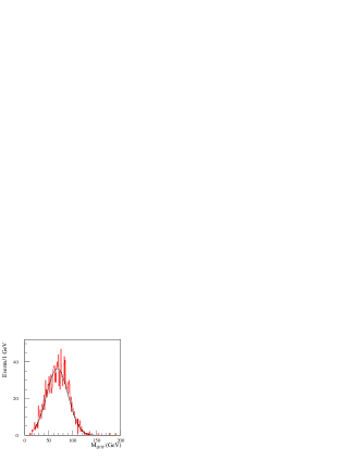
Fig. 38.: Invariant mass distribution $M_{lJ/\mathchar 265\relax}$, for five years of running at high luminosity.

Fig. 39.: Correlation the top mass and the $lJ/\mathchar 265\relax$ invariant mass $M_{lJ/\mathchar 265\relax}$.

The distribution fitted by a Gaussian leads to a mean $lJ/\mathchar 265\relax$ invariant mass of 68.1 GeV with a peak width of 22.4 GeV. The combinatorial background is small. For five years of running at high luminosity, the statistical error on $M_{lJ/\mathchar 265\relax}$ would be approximately 0.5 GeV. To improve the statistics, various strategies might be considered, such as for example removing the requirement of the muon-in-bjet and determine the final state topology by jet charge measurements. Nevertheless, further study is needed to evaluate the effectiveness of these approaches.

The correlation between the top mass and $lJ/\mathchar 265\relax$ invariant mass is shown on figure 39. One expects the uncertainties of the top mass to scale as a factor $1/0.58\simeq 1.7$ compared to the estimated errors on $M_{lJ/\mathchar 265\relax}$. Therefore, for five years of running at high luminosity, the statistical uncertainty on the top mass would approximately 0.8-0.9 GeV.

5.2 Background processes

The major sources of background come from processes involving $b\bar{b}$ production. Potential backgrounds such as W+jets, Z+jets and boson pair productions are briefly discussed.

The boson pair production processes (WW, WZ and ZZ) have small cross-sections compared to signal [33]. Furthermore, all the final states topologies are different with respect to the signal (except for one particular case but with tiny cross-sections [33]). These processes can be neglected.

The cross-sections for W+jets and Z+jets processes are about a factor of 20 higher or similar to the signal cross-section, respectively. Here also nevertheless, the final states are different with respect to the signal. These processes can be neglected as well.

The total cross-section for inclusive $b\bar{b}$ production is approximately $10^{6}$ larger than the signal cross-section. The final state is simply missing one isolated lepton compared to the signal. Taking into account the various branching ratios and for one year of running at high luminosity, of the order of $3.5\times 10^{9}b\bar{b}$ events with three non-isolated muons can be expected, compared to 2700 signal events. $10^{6}b\bar{b}$ events with three non-isolated muons have been generated. Only $2.9\%$ of the events are reconstructed with three non-isolated muons with $p_{T}>3\ \rm GeV$ and $|\eta|<2.4$. Only $0.05\%$ of the events are reconstructed with one isolated lepton with $p_{T}>30\ \rm GeV$ and $|\eta|<2.4$. No events survive when both of these requirements (corresponding to the signal selection cuts) are applied. In addition, a cut on the transverse missing energy could be applied ($p_{T}^{miss}>20\ \rm GeV$) which would reduce the $b\bar{b}$ rate by a factor of 6 and have no effect on the signal [33]. Therefore, and although more statistic would be helpful, the $b\bar{b}$ background process can probably be controlled.

The $Wb\bar{b}$ process has exactly the same final topology as the signal. The cross-section, for $W\rightarrow l\nu$, is approximately 85 pb [34]. After selection cuts, the reconstruction efficiency if $1.2\%$ ($16\%$ for the signal). Therefore, after selection cuts, the signal over background ratio would $S/B\approx 55$. This background process can also be controlled.

In conclusion, all the background processes are either negligible or can be kept under control.

5.3 Systematic uncertainties

This technique is insensitive to the jet energy scale which is the main source of systematic uncertainty in direct top mass measurements. However, the main limitation to a precise determination of the top mass using this method relies on how well the Monte Carlo describes the top production and decay. Particularly, the proper description of the fragmentation of the b hadrons is a crucial point.

The most relevant sources of systematic uncertainties have been investigated in the following. Shifts of $M_{lJ/\mathchar 265\relax}$ ($\mathchar 257\relax M_{lJ/\mathchar 265\relax}$) have been determined, defined as the difference between the value of $M_{lJ/\mathchar 265\relax}$ under nominal conditions and under the condition of the systematic uncertainty source, as described in the previous sections. Due to the huge amount of the required Monte Carlo statistics, the mass shifts have been obtained with a non negligible error [33]. Nevertheless, the quoted numbers should give a realistic estimate of the impact of the systematic uncertainty sources.

Fig. 40.: Dependence of the reconstructed $M_{lJ/\mathchar 265\relax}$ on the top quark transverse momentum.

The mass shifts obtained for initial state radiation, parton distribution function and the b-quark fragmentation parameter are summarized in table 12.

Source	Mass shift in GeV
ISR	0.1
PDF	0.2
$\epsilon_{b}\pm 10\%$	+0.4/0.0
$\epsilon_{b}\pm 20\%$	+0.8/0.1

Table 12.: $M_{lJ/\mathchar 265\relax}$ shifts for the various systematic uncertainties sources.

The $lJ/\mathchar 265\relax$ invariant mass can be determined with a systematic uncertainty of the order of 0.5 GeV which translates to a systematic error on the top mass of the order of 1 GeV.

5.4 Top transverse momentum:

The stability of $M_{lJ/\mathchar 265\relax}$ as a function of $p_{T}(top)$ has been controlled and a strong $p_{T}(top)$ dependence has been found, as shown on figure 40. This analysis has been repeated at generator level using the following selection criteria: no cut applied, cuts on isolated lepton only, cuts on non-isolated muons only, and all cuts applied. As expected, no dependence is observed when no cuts are applied. The cuts on the non-isolated muons introduces a small effect whereas the cuts on the isolated lepton has a strong impact [33]. This effect is a kinematic one. It can be kept under control as long as the Monte Carlo is well tuned to the data, which is needed in any case for the determination of the top mass from $M_{lJ/\mathchar 265\relax}$.

5.5 Summary

During the high luminosity phase of the LHC, the top quark mass can be determined in leptonic final states with $J/\mathchar 265\relax$. This indirect method relies heavily on the proper Monte Carlo description of the top production and decay. The top mass can be determined with both a statistical and systematic uncertainty at the level of 1 GeV.

6 Conclusion

The LHC will be an excellent place to study the top quark properties. The very large sample of top events that will be accumulated will allow a precision measurement of the top quark mass. Various methods applied to statistically independent samples gathering all dominant decay channels of the top quark have been investigated. The studies have shown that after only one year of data taking at low luminosity (per $10fb^{-1}$), a total error on the top mass at the level of 2 GeV can be achieved. In the inclusive lepton plus jets channels, the error can probably be further reduced down to 1 GeV. In all channels, the errors are dominated by systematic uncertainties (the systematic errors are summarized in table 13).

Source of error	Lepton+jets	Lepton+jets	Dilepton	All jets
in GeV	inclusive	large clusters		high pT
	sample	sample		sample
Energy scale
Light jet energy scale	0.2	-	-	0.8
b-jet energy scale	0.7	-	0.6	0.7
Mass scale calibration	-	0.9	-	-
UE estimate	-	1.3	-	-
Physics
Background	0.1	0.1	0.2	0.4
b-quark fragmentation	0.1	0.3	0.7	0.3
Initial state radiation	0.1	0.1	0.1	0.4
Final state radiation	0.5	0.1	0.6	2.8
PDF	-	-	1.2	-

Table 13.: Summary of the systematics errors in the top mass measurement, in the lepton plus jets channel, in the all jets channel and in the dilepton channel.

The analyses presented in this paper are differently sensitive to the various sources of systematic errors. This will allow reliable cross-checks between the various methods and an efficient extraction of the combined ATLAS measurement of the top quark mass.

In the inclusive lepton plus jets channel, errors are dominated by the b-jet energy scale and the knowledge of FSR. It was shown that these effects can be better controlled using a continuous jet definition. A possibility has been seen to reduce the systematic error due to the b-jet scale uncertainty by calibrating the b-jets with the same calibration as determined for light jets, though this must be further studied will full detector simulation before conclusions can be reached. In the lepton plus jets channel, using a sub-sample of hight $p_{T}$ top events, the top mass can be reconstructed with a large calorimeter cluster. In the all jets channels, it was demonstrated that the $t\bar{t}$ signal can be efficiently extracted from the huge QCD background. In the dilepton channel, it was presented that despite the two undetected neutrinos the final state can be fully reconstructed assuming a value for the top mass. Finally, during the high luminosity phase of the LHC, the top mass can also be precisely determined in leptonic final states with $J/\mathchar 265\relax$.

7 Acknowledgments

This work has been performed within the ATLAS Collaboration and we would like to thank collaboration members for helpful discussions. We are very grateful to Marina Cobal and John Parsons for their careful reading of the paper. We made use of the ATLAS physics simulation and analysis framework tools which are the fruit of a collaboration-wide effort.

References

- 1. A. Castro: FERMILAB-CONF-01/095-E. Proceedings of the 13th Convegno Sulla Fisica AL LEP (LEPTRE 2001), Rome, Italy (2001).
- 2. CDF II Detector Technical Design Report FERMILAB-pub-96/390-E.
- 3. CERN Yellow Report 2000-004, 9 may 2000, edited by G. Altarelli and M.L. Mangano, top physics chapter, page 23.
- 4. T. Lee, Heavy quark mass determination from the quarkonium ground state energy: a pole mass approach, JHEPJHEP10 (2003) 044.
- 5. M.C. Smith and S.S. Willenbrock, Phys. Rev. Lett. 79 (1997) 3825.
- 6. R. Bonciani et al., Nucl. Phys. B 529 (1998) 424.
- 7. ATLAS Collaboration: ATLAS Detector and Physics Performance Technical Design Report, CERN-LHCC-99-14-15 (1999).
- 8. T. Sjostrand, Computer Phycics Communication 82 (1994).
- 9. E. Richter-Was, D. Froidevaux and L. Poggioli, ATLFAST2.0 a fast simulation package for ATLAS., ATLAS Internal Note ATL-PHYS-98-131 (1998).
- 10. C. Biscarat, R. Lefevre, C. Santoni ’In Situ Jet Energy Calibration In The ATLAS Experiment’, proceedings of the 9th International Conference on Calorimetry in High Energy Physics, Annecy, France, 9-14 October 2000/Ed. by B. Aubert, J. Colas, P. Nédélec, L. Poggioli.
- 11. M. David, M. Cobal, A. De Angelis, A. Maio ’Measurement Of The Top Quark Mass With The ATLAS Detector At LHC’, ATLAS Internal Note ATL-COM-PHYS-2001-004
- 12. M. David, ’Systematic uncertainties on the determination of the top mass at the LHC/ATLAS from fragmentation effects’ PHD thesis, Universidade de Lisboa, October 2001
- 13. P. Roy, PHD thesis, Blaise Pascal University, PCCFT0202 (2002).
- 14. C. Peterson et al., Phys. Rev. D27 (1983) 105.
- 15. ALEPH Collaboration, Phys. Rep. 294 (1998) 1.
- 16. V. Kostioukhine, ATLAS Internal Note ATL-PHYS-2001-006.
- 17. F. Tkachev, ”Measuring multijet structure of hadronic energy flow or what is a jet?”, HEP-PH/9601308.
- 18. R. Maronna, ”Robust M-estimators of multivariate location and scatter”. The Annals of Statistics vol. 4 (1976) 51.
- 19. D.F. Andrews, ”A Robust method for multiple linear regression”. Technometrics vol. 16(1974) 4.
- 20. CDF Collaboration, Phys. Rev. D50(1994)2966; Phys. Rev. D51-(1995)4623; Phys. Rev. Lett. 74(1995)2626.
- 21. DØ Collaboration, Phys. Rev. Lett. 74(1995)2422.
- 22. I. Efthymiopoulos and F. Fassi, ATLAS Internal note ATL-COM-PHYS-99-050 (2002).
- 23. S. Aguvall et al. (ATLAS/TileCal Collaboration). ”Hadronic Shower Development in Iron-Scintillator Tile Calorimetry”. Nucl. Instr. and Meth., A443 (2000) 51-7, hep-ex/9904032.
- 24. I.Efthymiopoulos (ATLAS/TileCal Collaboration). ”Comparison between the ATLAS/TileCal hadron barrel calorimeter prototype test-beam data and hadronic simulation packages” VI International Conference on Calorimetry in High Energy Physics, Frascati, Italy, Jun. 1996. Published in the Proceedings of the conference, Frascati Physics Series, Vol V, pp 497-507.
- 25. T. A. Gabrial et al, Nucl. Inst. and Meth. A338 (1994) 336.
- 26. V. Šimák et al., ATLAS Internal note ATL-COM-PHYS-99-073 (1999).
- 27. F. Abe et al., CDF Collaboration, Phys. Rev. Lett. 79 (1997) 1992.
- 28. B. Abbot et al., DØ Collaboration, Phys. Rev. D 60 (1999) 012001; B. Abbot et al., DØ Collaboration, Phys. Rev. Lett. 83 (1999) 1908; hep-ex/9901023.
- 29. B. Abbott et al., DØ Collaboration, Phys. Rev. D 58 (1998) 052001.
- 30. J.M. Benlloch, N.Wainer, W.T. Giele, Phys. Rev. D 48 (1993) 5226.
- 31. L. Simic et al., ATLAS Internal note ATL-PHYS-2002-009 (2002).
- 32. CMS Letter of Intent, CERN/LHCC92-3 (1992) 90.
- 33. P. Grenier, ATLAS Internal note ATL-PHYS-2001-016 (2001).
- 34. B.P. Kersevan and E. Richter-Was, ATLAS Physics Communication ATL-COM-PHYS-2001-13.