Recent Results from D0

Abstract

We discuss recent ($B$ physics) results from D0. The results presented here correspond to an integrated luminosity of $\approx 115$ pb^-1 of data collected at the Tevatron, between April 2002 and June 2003, at a center of mass energy of ($p$ $\overline{p}$ collisions) of 1.96 TeV.

1 Introduction

The $B$ physics program at D0, is designed to be complementary to the program at the $B$-factories at SLAC and KEK and includes studies of $B_{s}$ oscillations, quarkonia (${J\mskip-3.0mu/\mskip-2.0mu\psi\mskip 2.0mu}$, $\chi_{c}$, $\mathchar 28935\relax$), searches for rare decays such as $B_{s}\rightarrow\mu^{+}\mu^{-}$, $B$ spectroscopy, e.g., $B^{*}_{sJ}$, lifetimes of the different $B$ hadrons, search for the lifetime difference in the $B_{s}$ CP eigenstates, study of beauty baryons, $B_{c}$, b production cross-section, etc.

One of the more important topics in $B$ physics is the search for $B_{s}$ $\kern 1.79993pt\overline{\kern-1.79993ptB}{}_{s}$ mixing. Global fits to the unitarity triangle, assuming that the Standard Model is correct, indicate that the 95% CL interval for the mixing parameter $\Delta M_{s}$ is (14.2-28.1)ps^-1 M. Battaglia (2003). The current limit is $\Delta M_{s}>14.9{\rm ps}^{-1}$ at the 95% CL M. Battaglia (2003). A measured value of $\Delta M_{s}$ much larger than the upper limits given here could pose a problem for the Standard Model.

2 D0 Detector

For the current run of the Tevatron (Run II), the D0 detector went through a major upgrade. The inner tracking system was completely revamped. The detector now includes a Silicon tracker, surrounded by Scintillating Fiber tracker, both of which are enclosed in a 2 Tesla solenoidal magnetic field. Pre-shower counters are located before the calorimeter to aid in electron and photon identification. The muon system has been improved, e.g. more shielding to reduce beam background was added.

The D0 detector has excellent tracking and lepton acceptance. Tracks with pseudo-rapidity ($\eta$) as large as 2.5–3.0 ($\theta\approx 10^{\circ}$) and transverse momentum (p_T) as low as 180 MeV/c are reconstructed.

The muon system can identify muons within $|\eta|<2.0$. The minimum p_T of the reconstructed muons varies as a function of $\eta$. In most of the results presented here, we required muons to have p${}_{T}>2$ GeV/c.

Low pT electron identification is currently limited to p${}_{T}>2$ GeV/c and $|\eta|<1.1$; however, we are working to improve both the momentum and $\eta$ coverage.

A Silicon based (hardware) trigger is being commissioned which will allow us to trigger on long-lived particles, such as the daughters of charm and beauty hadrons. We expect to start including this trigger in the online system after the current Tevatron shutdown ends in Mid-November. We are currently making impact parameter cuts at Level 3 (software trigger). The hardware trigger will allow us to make these cuts at an earlier stage.

3 Data Sample

The results presented here are based on data collected between April 2002 and June 2003. The dataset correspond to an integrated luminosity of about 115 pb^-1. We collected data with a dimuon as well as a single muon trigger. To reduce the data rate, a luminosity dependent prescale was applied to the single muon trigger (the prescale was 1 for instantaneous ${\cal L}<20\times 10^{30}{\rm cm}^{-2}{\rm s}^{-1}$). In both these triggers, the requirement that muons have hits in all layers of the muon system implies that they have total momentum $\geq 3$ GeV.

4 Results

$B_{s}$ oscillations is one of three processes where the flavour of the initial state changes by two units, the others being $K{\bar{K}}$ and $B^{0}_{d}{\bar{B}^{0}_{d}}$ mixing. Studies of $K{\bar{K}}$ mixing yielded results on indirect and direct CP violation, whereas the (unexpected) large value of $B^{0}_{d}{\bar{B}^{0}_{d}}$ mixing implied that the top quark was much heavier than expectations. If our current understanding of the Standard Model and the CKM matrix are correct, then $B_{s}$ oscillations should be in the allowed region, and any deviation could be a sign of new physics. If the mixing parameter, $\Delta M_{s}$ is very large then the difference in the widths of the CP eigenstates of the $B_{s}$ may be detectable.

The significance of a $B$ mixing measurement can be expressed as,

$${\rm Sig.}=\sqrt{\frac{N\epsilon D^{2}}{2}}\exp^{-(\Delta M_{s}\times\sigma_{t})^{2}/2}\sqrt{\frac{S}{S+B}}$$ (1)

where $N$ is the number of reconstructed $B_{s}$ events, $\epsilon D^{2}$ is a measure of how well we know the flavour of the $B_{s}$ at production, $\sigma_{t}$ is the proper time resolution, and $S/(S+B)$ expresses the cleanliness of the signal.

To study $B_{s}$ oscillations we therefore need three ingredients, (a) final state reconstruction, (b) ability to measure $B$ decay lengths, and (c) flavour tagging of the $B$ both at production and decay.

4.1 Final State Reconstruction

We can reconstruct $B_{s}$ in both the hadronic and semi-leptonic final states. The advantage of the former is that since it is a fully reconstructed decay, the proper time resolution is much better, whereas the branching fraction for the latter is much larger ($\approx 10\%$ vs. 0.5%).

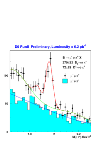
Figure 1: $B_{s}$ semi-leptonic yield

In Fig. 1 we show the $B_{s}\rightarrow D_{s}\mu X$ signal for ${\int{\cal L}}\approx 6.2$ pb^-1. The blue shaded histogram represents the wrong sign combinations. By comparison, we expect to see about 1.0 $B_{s}\rightarrow D_{s}\pi$ events/pb^-1.

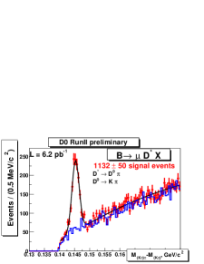
Figure 2: $B\rightarrow D^{*-}\mu X$

In Figure 2, we present the inclusive $B\rightarrow D^{*-}\mu X$ signal for ${\int{\cal L}}\approx 6.2$ pb^-1. The blue line represents the wrong sign combinations. We can use this mode to study $B^{0}_{d}$ mixing and for measuring inclusive $B$ lifetime.

We will also reconstruct hadronic $B_{s}$ decays, e.g., $B_{s}\rightarrow D_{s}\pi$, as well as semi-electronic final states. Details about $B$ hadron reconstruction at D0 can be found in E. Von Toerne’s contribution to these proceedings.

4.2 Lifetime Measurement

In Fig. 3, we present a measurement of the inclusive $B$ lifetime using $B\rightarrow D^{0}\mu X$ decays.

The background shape is obtained from the $D^{0}$ mass sidebands. Both sidebands and the signal regions are fitted with a combination of a Gaussian function to represent zero-lifetime background and exponentials (convoluted with Gaussian resolutions functions) to represent non-zero lifetime (the convolution is to take account of the smearing).

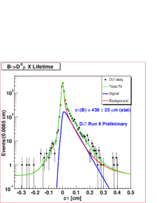
Figure 3: Lifetime for $B\rightarrow D^{0}\mu X$

From the fit, we measure the inclusive $B$ lifetime to be $438\pm 25({\rm stat.})$ $\mu{\rm m}$, which agrees with the world average, $472\pm 2$ $\mu{\rm m}$ K. Hagiwara (2002). We have also measured lifetimes for other $B$ hadrons, and details can be found in Daria Zieminska’s contribution to these proceddings.

4.3 Flavour Tagging

To be able to do a mixing measurement, one needs to know the flavour of the $B$ hadron at the time of production and decay. By using flavour-specific decays, one can easily tag the flavour at the time of decay. Tagging the $B$ flavour at production is more work. At D0, we plan to use the following techniques,

• Soft Lepton Tagging: The sign of the lepton produced in the semi-leptonic decay of the other $B$ in the event is used to tag the flavour of the other $B$. We then make the assumption that the flavour of the decay $B$ is opposite to that of the tag $B$. There will be some contamination due to the fact that the other $B$ can mix, or that we pick up the tag lepton from a charm semi-leptonic decay. This method has low efficiency, but very high tagging power. We also plan to use electrons.

• Jet Charge Tagging: We take all tracks opposite to the decay $B$ and form a track jet. The assumption is that these tracks are produced in the fragmentation of the other b-quark, as well as in the decay of the other $B$ hadron. This method has high efficiency, but has poorer tagging power.

• Same Side Tagging: In this technique, we identify tracks produced in the fragmentation of the b-quark which gives rise to the decay $B$. In addition, the decay B can come from a resonance, e.g., B${}^{**+}\rightarrow B^{0}\pi^{+}$, and one can use such pions to identify the flavour of the decay B at the time of production. This method has high efficiency, but has poorer tagging power

We benchmarked these techniques using a sample of $B^{+}\rightarrow{\rm J}/\psi{\rm K}^{+}$ decays. Since the $B^{+}$ does not oscillate, it provides for a good testing ground.

In Figure 4, we show the $B^{+}$ peak for all events, events with a (jet-charge) tag, and events with the correct tag. We use the fits to these peaks to determine the efficiency ($\epsilon$) and tagging power (Dilution) of the various techniques. $\epsilon=(N_{R}+N_{W})/N_{all}$, and Dilution = $(N_{R}-N_{W})/(N_{R}+N_{W})$, where $N_{all}$, $N_{R}$ and $N_{W}$ are the number of all events, correctly tagged and wrongly tagged events, respectively.

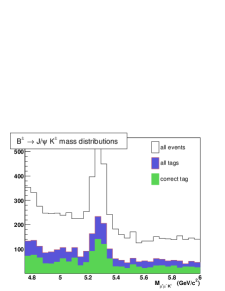
Figure 4: Fits for Jet Charge tagging results

The results for the various techniques are summarized in Table 1. We are in the process of checking these results on a sample of $B_{s}$ and $B^{0}$ events.

	$\epsilon$	Dilution(D)	$\epsilon D^{2}$
Soft Muon	5%	57%	$1.6\pm 1.1$%
Jet Charge	47%	27%	$3.3\pm 1.7$%
Same Side	79%	26%	$5.5\pm 2.0$%

Table 1: Summary of flavour tagging results

4.4 $B_{s}$ mixing

We expect to observe the following four classes of events,

• $B_{s}\rightarrow D_{s}\mu X$ collected with the single muon trigger. The flavour at production will be tagged using all three techniques discussed above.

• $B_{s}\rightarrow D_{s}\pi$ collected with the single muon trigger. In this case, we can use the trigger muon as the flavour tag. The tagging power will be very high in this case.

• $B_{s}\rightarrow D_{s}\mu X$ collected with the dimuon trigger. The flavour at production will be tagged using the second muon in the event.

• $B_{s}\rightarrow D_{s}eX$ collected with the single muon trigger. The flavour at production will be tagged using the trigger muon.

The semi-leptonic events have poorer proper time resolution compared to the hadronic mode, but much larger statistics. We are in the process of improving our estimate of the proper time resolution for both hadronic and semi-leptonic events. In addition, we can combine all modes to get a better measurement or a better limit.

If, we assume a resolution of $\approx 150$ fs, we project that using the first class of events (with $\int{\cal L}\approx 500$ pb^-1), we can make a 3$\sigma$ measurement if $\Delta M_{s}\approx 12$ ps^-1 or a 1.5$\sigma$ measurement if $\Delta M_{s}\approx 15$ ps^-1. The third and fourth class of events have a very similar reach in $\Delta M_{s}$.

For hadronic events (with the same luminosity), if the resolution is $\approx 110$ fs, the corresponding numbers are a 3$\sigma$ measurement if $\Delta M_{s}\approx 12$ ps^-1 or a 2.2$\sigma$ measurement if $\Delta M_{s}\approx 15$ ps^-1.

4.5 Quarkonia

At the Tevatron, J/$\psi$ can be produced either promptly (direct as well as indirect), i.e., $p\overline{p}\rightarrow{\rm J}/\psi({\rm or}\chi_{c}\rightarrow{\rm J}/\psi)$ or as a product in $B$ decays. $\mathchar 28935\relax$ by contrast are only produced promptly. The study of quarkonia sheds light on the strong interaction, especially non-perturbative QCD

In Run I (at the Tevatron), the production cross-section of direct J/$\psi$ was about 50 times larger than the Color Singlet Model.

With the new dataset, we plan to update the results on J/$\psi$ production cross-section as a function of $p_{T}$ and $\eta$, as well as study polarization effects. In addition, we are working to measure the absolute cross-section and polarization of the $\mathchar 28935\relax$ states.

5 Conclusions

The D0 detector has started to produce results in the field of $B$ physics. We currently have $\approx 220$ pb^-1 of data on tape, and expect to get up to $\approx 500$ pb^-1 by the end of 2004.

As a stepping stone to $B_{s}$ mixing, we plan to measure $\Delta M_{d}$ to benchmark our analyses techniques. In addition, we are pursuing a vigorous program, which includes measurement of $B$ lifetimes, rare decays, studies of quarkonia, beauty baryons, $B_{c}$, etc.

References

- M. Battaglia (2003) M. Battaglia, etal., The CKM matrix and the unitarity triangle, Tech. rep., arXiv:hep-ph/0304132 (2003).
- K. Hagiwara (2002) K. Hagiwara, etal., Physical Review D, 66, 1 (2002).