Improved measurement of the branching ratio of $J/\psi\rightarrow K_{S}^{0}K_{L}^{0}$

Abstract

The branching ratio of $J/\psi\rightarrow K_{S}^{0}K_{L}^{0}$ is measured with improved precision to be ${\cal B}(J/\psi\rightarrow K_{S}^{0}K_{L}^{0})=(1.82\pm 0.04\pm 0.13)\times 10^{-4}$ using $J/\psi$ data collected with the Beijing Spectrometer (BESII) at the Beijing Electron-Positron Collider. This result is used to test the perturbative QCD “12%” rule between $\psi(2S)$ and $J/\psi$ decays and to investigate the relative phase between the three-gluon and one-photon annihilation amplitudes in $J/\psi$ decays.

I Introduction

I.1 Decays of $J/\psi\rightarrow K_{S}^{0}K_{L}^{0}$

The decays of the $J/\psi$ into light hadronic final states can proceed via either three-gluon or one-photon annihilations, and it has been determined that the phases of these amplitudes are nearly orthogonal in many two-body exclusive decays, such as Vector-Pseudoscalar (VP), Vector-Vector (VV), Pseudoscalar-Pseudoscalar (PP) and Nucleon anti-Nucleon (N$\overline{\hbox{N}}$) suzuki ; dm2exp ; mk3exp ; a00 ; a11 ; ann . For the PP phase analysis, the $\pi^{+}\pi^{-}$, $K^{+}K^{-}$, and $K_{S}^{0}K_{L}^{0}$ decay branching ratios are required haber ; a00 ; a11 . The available $J/\psi\rightarrow K_{S}^{0}K_{L}^{0}$ branching ratios come from DMII dm2exp and MARKIII mk3pp ; these measurements have relative errors of about 18%. Here we report a measurement of the $K_{S}^{0}K_{L}^{0}$ decay branching fraction using the $J/\psi$ data sample collected with the Beijing Spectrometer (BESII) at the Beijing Electron-Positron Collider (BEPC).

Furthermore, there is a prediction of the relation between $J/\psi$ and $\psi(2S)$ decay branching ratios to the same hadronic final state ($h$) applequist ; franklin , that is

$$Q_{h}=\frac{{\cal B}(\psi(2S)\rightarrow h)}{{\cal B}(J/\psi\rightarrow h)}=\frac{{\cal B}(\psi(2S)\rightarrow e^{+}e^{-})}{{\cal B}(J/\psi\rightarrow e^{+}e^{-})}\approx 12\%.$$

While some channels obey the so called “12% rule”, others violate this rule very badly franklin ; wangwf . Thus it is interesting to test this rule for $K_{S}^{0}K_{L}^{0}$ decay, which can only be produced through SU(3) symmetry-breaking, strong decays of these charmonium states.

I.2 The experiment

The data used for this analysis are taken with the BESII detector at the BEPC storage ring at a center-of-mass energy corresponding to $M_{J/\psi}$. The data sample corresponds to a total of $57.7(1\pm 4.7\%)\times 10^{6}$ $J/\psi$ decays, as determined from inclusive 4-prong hadrons fangss .

BES is a conventional solenoidal magnet detector that is described in detail in Ref. bes ; BESII is the upgraded version of the BES detector bes2 . A 12-layer vertex chamber (VC) surrounding the beam pipe provides trigger information. A forty-layer main drift chamber (MDC), located radially outside the VC, provides trajectory and energy loss ($dE/dx$) information for charged tracks over $85\%$ of the total solid angle. The momentum resolution is $\sigma_{p}/p=0.017\sqrt{1+p^{2}}$ ($p$ in $\hbox{\rm GeV}/c$), and the $dE/dx$ resolution for hadron tracks is $\sim 8\%$. An array of 48 scintillation counters surrounding the MDC measures the time-of-flight (TOF) of charged tracks with a resolution of $\sim 200$ ps for hadrons. Radially outside the TOF system is a 12 radiation length, lead-gas barrel shower counter (BSC). This measures the energies of electrons and photons over $\sim 80\%$ of the total solid angle with an energy resolution of $\sigma_{E}/E=22\%/\sqrt{E}$ ($E$ in GeV). Outside of the solenoidal coil, which provides a 0.4 Tesla magnetic field over the tracking volume, is an iron flux return that is instrumented with three double layers of counters that identify muons of momentum greater than 0.5 GeV/$c$.

I.3 Monte Carlo

A Monte Carlo simulation is used for the determinations of the mass resolution and detection efficiency. This program (SIMBES), which is Geant3 based, simulates the detector response, including the interactions of secondary particles with the detector material. Reasonable agreement between data and Monte Carlo simulation has been observed in various channels tested, including $e^{+}e^{-}\rightarrow(\gamma)e^{+}e^{-}$, $e^{+}e^{-}\rightarrow(\gamma)\mu^{+}\mu^{-}$, $J/\psi\rightarrow p\overline{p}$ and $\psi(2S)\rightarrow\pi^{+}\pi^{-}J/\psi,J/\psi\rightarrow\ell^{+}\ell^{-}$ $(\ell=e,\mu)$.

For the signal channel, $J/\psi\rightarrow K_{S}^{0}K_{L}^{0}$, the angular distribution of the $K_{S}^{0}$ or $K_{L}^{0}$ is generated as $\sin^{2}\theta$, where $\theta$ is the polar angle in the laboratory system. The $K_{L}^{0}$ is allowed to decay and to interact with the detector material, and for the $K_{S}^{0}$, only $K_{S}^{0}\rightarrow\pi^{+}\pi^{-}$ is generated. For this study, 50,000 events are generated. A Monte Carlo sample with 30 M inclusive $J/\psi$ decays generated with Lundcharm lundcharm is used for background estimation.

II Event selection

For the decay channel of interest, the candidate events must satisfy the following selection criteria:

1. Two charged tracks with net charge zero are required.

2. Each track should satisfy $|\cos\theta|<0.80$, where $\theta$ is the polar angle in the MDC, and have a good helix fit so that the error matrix from track fitting is available for secondary vertex finding.

3. To remove backgrounds mainly from $J/\psi\rightarrow\overline{K}^{*}(892)^{0}K^{0}+c.c.$, $E_{\gamma}^{lft}<0.1$ GeV is required, where $E_{\gamma}^{lft}$ is the sum of the energies of the photon candidates outside a cone about the direction of the $K_{L}^{0}$ ($\cos\theta<0.95$). A neutral cluster is considered to be a photon candidate when the angle between the nearest charged track and the cluster in the $xy$ plane is greater than $15^{\circ}$, the first energy deposit is in the beginning 6 radiation lengths, and the angle between the cluster development direction in the BSC and the photon emission direction in the $xy$ plane is less than $37^{\circ}$.

The two tracks are assumed to be $\pi^{+}$ and $\pi^{-}$. To find the intersection of the two tracks near the interaction point, an iterative, nonlinear least squares technique is used wangzhe . The intersection is taken as the $K_{S}^{0}$ vertex, and the momentum of the $K_{S}^{0}$ is calculated at this point. Figure 1 shows a scatter plot of the $\pi^{+}\pi^{-}$ invariant mass versus the decay length in the transverse plane ($L_{xy}$) for events that satisfy the above selection criteria and have a $K_{S}^{0}$ momentum between 1.45 and 1.50 GeV/$c$. The cluster of events with mass consistent with the nominal $K_{S}^{0}$ mass and with a long decay length indicates a clear $K_{S}^{0}$ signal.

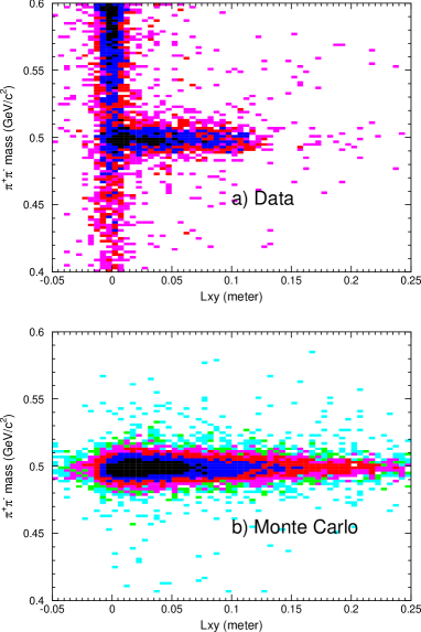
Figure 1: Scatter plot of $\pi^{+}\pi^{-}$ invariant mass versus the decay length in the transverse plane for events with $K_{S}^{0}$ momentum between 1.45 and 1.50 GeV/$c$ for a) data and b) Monte Carlo simulation.

Figure 2 shows the $\pi^{+}\pi^{-}$ invariant mass distributions of both data and Monte Carlo simulation. A fit with a Gaussian and a second order polynomial background gives a $K_{S}^{0}$ mass of $(499.3\pm 0.2)~{}\hbox{MeV}/c^{2}$ and mass resolution of $(6.5\pm 0.2)~{}\hbox{MeV}/c^{2}$ for data, while the corresponding numbers are $(499.0\pm 0.1)~{}\hbox{MeV}/c^{2}$ and $(6.04\pm 0.05)~{}\hbox{MeV}/c^{2}$ for Monte Carlo simulation. The masses for data and Monte Carlo simulation agree well, although both of them deviate from the world average mass $(497.672\pm 0.031)~{}\hbox{MeV}/c^{2}$ pdg . The mass resolution from Monte Carlo simulation is smaller than that of data.

Figure 2: The $\pi^{+}\pi^{-}$ invariant mass distributions for a) data and b) Monte Carlo simulation.

Figure 3 shows the comparison of the $K_{S}^{0}$ decay length distributions between data and Monte Carlo simulation after normalizing the Monte Carlo data to the number of events with $2<L_{xy}<10$ cm. The discrepancy below 1 cm indicates the still remaining non-$K_{S}^{0}$ background events in the sample. The difference at $L_{xy}>11$ cm will be discussed later.

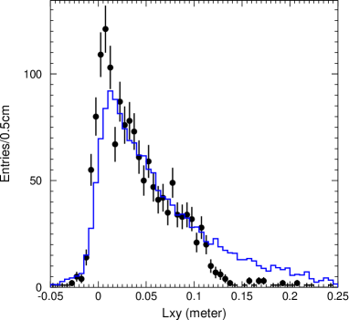
Figure 3: Comparison of the $K_{S}^{0}$ decay length distributions between data and Monte Carlo simulation after normalizing the Monte Carlo data to the number of events with $2<L_{xy}<10$ cm.

After requiring $L_{xy}>1$ cm and the $\pi^{+}\pi^{-}$ mass within twice the mass resolution around the nominal $K_{S}^{0}$ mass and removing the $\gamma$ conversion background (described later), the $K_{S}^{0}$ momentum distribution is shown in Figure 4. In the plot, there is a clear peak around 1.46 GeV/$c$ corresponding to $J/\psi\rightarrow K_{S}^{0}K_{L}^{0}$ decays, and another peak around 1.37 GeV/$c$ corresponding to $J/\psi\rightarrow\overline{K}^{*}(892)^{0}K^{0}+c.c.$. The background, as estimated from the $K_{S}^{0}$ mass side bands (three sigma away from the $K_{S}^{0}$ nominal mass on both sides), can explain the contribution in the high momentum region, while in the lower momentum region, there are additional backgrounds due to other channels with $K_{S}^{0}$ production.

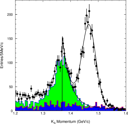
Figure 4: The $K_{S}^{0}$ momentum distribution for data after the final selection. Dots with error bars are data, the dark shaded histogram is from $K_{S}^{0}$ mass sideband events, and the light shaded histogram is the Monte Carlo simulated background. The curve shown in the plot is from a best fit of the distribution.

The secondary vertex requirement and invariant mass cut are very effective in reducing backgrounds from non-$K_{S}^{0}$ events. However since there is no particle identification requirement for the tracks used, there is contamination from $e^{+}e^{-}\rightarrow\gamma\gamma$ where one photon converts into an $e^{+}e^{-}$ pair which passes the above selection criteria. This background can be seen in Figure 5, where the total BSC energy versus the total momentum of the charged tracks is shown. The events with high total momentum and large BSC energies in the upper right corner of the figure are due to this gamma conversion background.

Figure 5: The total BSC energy of the two charged tracks versus the momentum of the $K_{S}^{0}$. The cluster in the upper right corner is due to gamma conversion background.

Figure 6 shows a scatter plot of the total BSC energy versus the total $XSE$ (difference from the expected $dE/dx$ for the electron hypothesis divided by the $dE/dx$ resolution) of the two charged tracks for events with $K_{S}^{0}$ momentum larger than 1.45 GeV/$c$ for both data and Monte Carlo simulation. It can be seen that requiring a total BSC energy greater than 1.0 GeV and total $XSE$ greater than $-4$ will select almost all the gamma conversion background, while the efficiency of this cut for the signal is very high (about 99.0% according to Monte Carlo simulation).

Figure 6: The scatter plot of the total BSC energy versus the total $XSE$ of the two charged tracks with $K_{S}^{0}$ momentum larger than 1.45 GeV/$c$ for both data (upper) and Monte Carlo simulation (lower). The cluster in the upper right corner for data is due to gamma conversions.

Figure 7 shows the distributions of events identified as gamma conversions for data and Monte Carlo simulated signal events. There is no indication of signal in the expected momentum region for $J/\psi\rightarrow K_{S}^{0}K_{L}^{0}$ events.

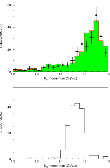
Figure 7: The $K_{S}^{0}$ momentum distribution of events identified as gamma conversions. Events in the $K_{S}^{0}$ mass signal region are shown by dots with error bars and the events in $K_{S}^{0}$ mass sidebands are shown by the shaded histogram in the upper plot for data, and the Monte Carlo simulation of $J/\psi\rightarrow K_{S}^{0}K_{L}^{0}$ is shown in the lower plot.

The $\gamma$ conversion events can also be removed by cutting on the the opening angle between the two charged tracks; a requirement that the opening angle be larger than $20^{\circ}$ removes about the same fraction of background events with about the same efficiency for signal events as the cuts used above. This indicates the reliability of the cuts used for gamma conversion rejection.

Since there is no photon production in $K_{S}^{0}K_{L}^{0}$ events, one expects no photons reconstructed in the candidate events. However the $K_{L}^{0}$ may decay in the detector, and the decay products or hadronic interactions of the $K_{L}^{0}$ with the detector material can produce clusters in the shower counter. As a check, we required the number of photon candidates in the event to be zero (about 45% of $K_{S}^{0}K_{L}^{0}$ events satisfy this cut according to Monte Carlo simulation). Figure 8 shows the $K_{S}^{0}$ momentum distribution after this cut. It is clear that the background level, including the peak corresponding to $J/\psi\rightarrow\overline{K}^{*}(892)^{0}K^{0}+c.c.$, is greatly reduced, while the peak at high momentum is lowered by about a factor of two as expected from Monte Carlo simulation.

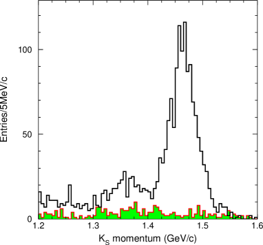
Figure 8: The $K_{S}^{0}$ momentum distribution for events without extra photons (blank histogram). The $K_{S}^{0}$ sideband background is shown by the shaded histogram.

III Backgrounds

III.1 Continuum background

$K_{S}^{0}K_{L}^{0}$ production via virtual photon annihilation is forbidden under SU(3) symmetry. This is checked by applying the same selection criteria to the data sample taken below the $J/\psi$ peak, at $\sqrt{s}=3.0$ GeV. This data was taken during the $J/\psi$ data taking, and the integrated luminosity is measured to be ${\cal L}=0.7~{}\hbox{pb}^{-1}$.

The $K_{S}^{0}$ momentum spectrum of the selected events is shown in Figure 9; the events in the signal region agree well with the expectation from the $K_{S}^{0}$ mass sidebands. As a conservative estimation, we take all the events with momentum within two standard deviation from the central value predicted by the Monte Carlo as signal to set the upper limit on the production cross section. For the two observed $e^{+}e^{-}\rightarrow K_{S}^{0}K_{L}^{0}$ candidates, the upper limit on the cross section at the 90% C. L. is

$$\sigma<35~{}\hbox{pb}.$$

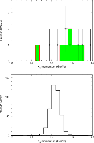
Figure 9: The $K_{S}^{0}$ momentum distributions for data (upper) and Monte Carlo simulation (below) at $\sqrt{s}=3.0$ GeV. The dots with error bars are data, and the shaded histogram in the upper plot is from the $K_{S}^{0}$ mass sidebands.

The integrated luminosity of the $J/\psi$ data sample is estimated to be around 17.8 pb^-1 fangss , approximately 25 times as large as the continuum sample. Since the efficiencies for detecting $K_{S}^{0}K_{L}^{0}$ at the $J/\psi$ and at $\sqrt{s}=3.0$ GeV are about the same, we estimate the continuum contribution of $K_{S}^{0}K_{L}^{0}$ at the $J/\psi$ to be at most 50 events, which is small compared to the number of events observed at the $J/\psi$ (more than 2000). Since the lack of evidence for $K_{S}^{0}K_{L}^{0}$ production from the continuum agrees well with the SU(3) symmetry prediction, this contribution is neglected in the following analysis.

III.2 Backgrounds from inclusive $J/\psi$ decays

Figure 10 shows the $K_{S}^{0}$ momentum spectrum obtained for the inclusive Monte Carlo events after all cuts and after normalizing to the total number of $J/\psi$ events. It can be seen that there are also two peaks at the expected positions for $\overline{K}^{*}(892)^{0}K^{0}+c.c.$ and $K_{S}^{0}K_{L}^{0}$ as has been observed with data. The Monte Carlo simulation reproduces the shape of the peaks, but is lower than the data. This indicates the branching ratios used in the Monte Carlo simulation are too low. The branching fraction of $J/\psi\rightarrow K_{S}^{0}K_{L}^{0}$ in the generator is $7.8\times 10^{-5}$, and that of $J/\psi\rightarrow\overline{K}^{*}(892)^{0}K^{0}+c.c.$ is $5.08\times 10^{-3}$.

Figure 10: Comparison of the $K_{S}^{0}$ momentum distributions between data (dots with error bars) and the inclusive Monte Carlo sample (histogram), normalized to the total number of $J/\psi$ events.

The main background in the intermediate $K_{S}^{0}$ momentum region is due to $J/\psi\rightarrow\overline{K}^{*}(892)^{0}K^{0}+c.c.$ where the $K^{*0}$ decays into $K^{0}$ and a $\pi^{0}$, and one $K^{0}$ becomes a $K_{S}^{0}$ and the other becomes a $K_{L}^{0}$. Another potential background is due to $J/\psi\rightarrow\rho^{0}\pi^{0}$, which has a large branching ratio, but this background is included in the $K_{S}^{0}$ side band events. The background from $J/\psi\rightarrow\gamma\eta_{c}$, with $\eta_{c}$ decaying into final states containing a $K_{S}^{0}$ can also contaminate the signal, but this background is small because $\eta_{c}$ production is two orders of magnitude lower than $J/\psi$.

Figure 4 shows the $K_{S}^{0}$ momentum distribution for the background channels with the input branching fraction of $J/\psi\rightarrow\overline{K}^{*}(892)^{0}K^{0}+c.c.$ taken to be $(5.2\pm 0.5)\times 10^{-3}$, obtained from a preliminary analysis of the same data sample, together with the contribution from the $K_{S}^{0}$ mass side band events. The agreement between the background estimation and data is good below the $K_{S}^{0}K_{L}^{0}$ peak, indicating the estimation of the background under the $K_{S}^{0}K_{L}^{0}$ peak is reliable. The discrepancy at lower momentum indicates backgrounds from other channels (like $J/\psi\rightarrow K^{*}(892)^{0}\overline{K^{*}_{0}}(1430)^{0}+c.c.$, $J/\psi\rightarrow K^{*}(892)^{0}\overline{K^{*}_{2}}(1430)^{0}+c.c.$, etc.), which are not generated in this comparison, are important, but they do not affect the results in the signal region.

IV Fit of the momentum spectrum

The $K_{S}^{0}$ momentum spectrum of the selected events is fitted from 1.37 to 1.60 GeV/$c$ with a Gaussian distribution for the signal, a constant term for the non-$K_{S}^{0}$ background, and an exponential term for the background from $J/\psi\rightarrow\overline{K}^{*}(892)^{0}K^{0}+c.c.$ using an unbinned maximum likelihood method. The fit results are shown in Figure 4; the backgrounds from the $K_{S}^{0}$ mass side bands and the $J/\psi\rightarrow\overline{K}^{*}(892)^{0}K^{0}+c.c.$ background, also shown, agrees well with the fitted background. The fitted $K_{S}^{0}$ momentum peak is at $(1466.2\pm 0.7)$ MeV/$c$, which agrees well with the expectation of $1466.3$ MeV/$c$. The fitted momentum resolution is $(25.2\pm 0.7)$ MeV/$c$, which is in good agreement with that of the Monte Carlo simulation, $(24.4\pm 0.2)$ MeV/$c$. The fit yields $2155\pm 45$ events, and the efficiency for detecting $J/\psi\rightarrow K_{S}^{0}K_{L}^{0}$, with $K_{S}^{0}\to\pi^{+}\pi^{-}$ is $(38.69\pm 0.23)\%$ from the Monte Carlo simulation.

V Efficiency corrections and systematic errors

The systematic error in the branching ratio measurement comes from uncertainties in the efficiencies of the photon energy cut, secondary vertex finding, MDC tracking, and the trigger; the branching ratios used; the number of $J/\psi$ events; the $K_{S}^{0}$ mass cut; the angular distributions; etc.

V.1 Photon energy cut

According to the Monte Carlo simulation, the $E_{\gamma}^{lft}$ cut has an efficiency of 93.6% for $J/\psi\rightarrow K_{S}^{0}K_{L}^{0}$ events, while many backgrounds are removed. The energy is produced in signal events by the decays and hadronic interactions of the $K_{L}^{0}$ with the detector material; the simulation of this effect depends strongly on the detector simulation software. This is checked with the $J/\psi\rightarrow K_{S}^{0}K_{L}^{0}$ signal, requiring the $K_{S}^{0}$ momentum greater than 1.45 GeV/$c$ and less than 1.50 GeV/$c$. This cut removes almost all the contamination from $J/\psi\rightarrow\overline{K}^{*}(892)^{0}K^{0}+c.c.$. The $E^{lft}_{\gamma}$ distributions of both data and Monte Carlo simulation, which agree well, are shown in Figure 11. The efficiency for data is found to be $(99.4\pm 0.7)\%$ of that for Monte Carlo simulation. No correction to the final efficiency is performed, and 1.5% is taken as the systematic error of this cut.

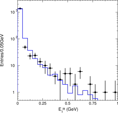
Figure 11: Comparison of the $E^{lft}_{\gamma}$ distributions for $J/\psi\rightarrow K_{S}^{0}K_{L}^{0}$ events with $K_{S}^{0}$ momentum greater than 1.45 GeV/$c$ and less than 1.50 GeV/$c$ between data (dots) and Monte Carlo simulation (histogram), normalized to the total number of events. The contribution of sideband events has been subtracted from data.

V.2 Secondary vertex finding

The efficiency of the secondary vertex finding algorithm has been checked using $J/\psi\rightarrow\overline{K}^{*}(892)^{0}K^{0}+c.c.$ events, where the $K_{S}^{0}$ has a momentum around 1.37 GeV/$c$, and $J/\psi\rightarrow\overline{K}^{*}(892)^{-}K^{+}+c.c.$ events, where the $K_{S}^{0}$ momentum is between 0.4 and 1.4 GeV/$c$. The study shows that the Monte Carlo simulates data (with $L_{xy}>1.0$ cm) fairly well. Figure 12 shows the ratio of the $K_{S}^{0}$ reconstruction efficiencies of data and Monte Carlo simulation as a function of the $K_{S}^{0}$ momentum. Fitting the points with a second order polynomial and extrapolating to the $K_{S}^{0}$ momentum for $J/\psi\rightarrow K_{S}^{0}K_{L}^{0}$ a correction factor to the efficiency from the Monte Carlo simulation can be obtained.

Figure 12: The ratio of the $K_{S}^{0}$ reconstruction efficiencies of data and Monte Carlo simulation as a function of the $K_{S}^{0}$ momentum; the curve shows the best fit to the points using a second order polynomial.

The polar angle dependence of the $K_{S}^{0}$ reconstruction efficiency has also been studied with the above sample. Figure 13 shows the ratio between the $K_{S}^{0}$ reconstruction efficiencies of data and Monte Carlo simulation as a function of the cosine of the $K_{S}^{0}$ polar angle. Reweighting the efficiency by the expected angular distribution of the $K_{S}^{0}$ in $J/\psi\rightarrow K_{S}^{0}K_{L}^{0}$ another correction factor to the efficiency determined by the Monte Carlo simulation can be obtained.

Figure 13: The ratio between the $K_{S}^{0}$ reconstruction efficiencies of data and Monte Carlo simulation as a function of the $K_{S}^{0}$ polar angle.

Combining the above two effects, a correction of $(96.4\pm 3.1)\%$ to the Monte Carlo efficiency is obtained. The error, comes from the extrapolation and the limited statistics of the samples used, will be taken as the systematic error of the secondary vertex finding.

V.3 MDC tracking

The MDC tracking efficiency has been measured using channels like $J/\psi\rightarrow\Lambda\overline{\Lambda}$ and $\psi(2S)\rightarrow\pi^{+}\pi^{-}J/\psi$, $J/\psi\rightarrow\mu^{+}\mu^{-}$. It is found that the efficiency of the Monte Carlo simulation agrees with that of data within 1-2% per charged track. Therefore 4% will be taken as the systematic error on the tracking efficiency for the channel of interest. When the $\pi$ momentum spectrum of the selected $J/\psi\rightarrow K_{S}^{0}K_{L}^{0}$ events is compared with that of the Monte Carlo simulation, good agreement between data and Monte Carlo simulation is observed in the full momentum range.

V.4 Trigger efficiency

The trigger condition which strongly affects the $K_{S}^{0}K_{L}^{0}$ efficiency is the requirement of hits in the Vertex Chamber zhaodx , since for the $K_{S}^{0}$ of interest, the momentum is high (1.466 GeV/$c$ for $J/\psi\rightarrow K_{S}^{0}K_{L}^{0}$) and the decay length $\gamma\beta c\tau$, is 7.9 cm, while the outer radius of the VC is 13.5 cm. Figure 3 shows the $K_{S}^{0}$ decay length in the $xy$-plane of $J/\psi\rightarrow K_{S}^{0}K_{L}^{0}$ decays. There is a sudden drop of efficiency at around $L_{xy}=11-12$ cm for data, which is not seen with the Monte Carlo sample, since no trigger simulation is included in the current version of the Monte Carlo. Normalizing the Monte Carlo events to the data with $L_{xy}$ between 1 cm and 10 cm and comparing the number of events for all $L_{xy}$ with the Monte Carlo, yields a correction factor of $(80.1\pm 0.8)\%$ to the Monte Carlo efficiency for $J/\psi\rightarrow K_{S}^{0}K_{L}^{0}$.

V.5 Angular distribution

Figure 14 shows the cosine of the $K_{S}^{0}$ polar angle for $K_{S}^{0}K_{L}^{0}$ events from $J/\psi$ decays; good agreement between data and Monte Carlo simulation is observed. This indicates that the input angular distribution in the Monte Carlo generator is correct.

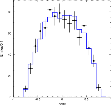
Figure 14: Cosine of the $K_{S}^{0}$ polar angle of $K_{S}^{0}K_{L}^{0}$ events from $J/\psi$ decays. Dots with error bars are data, and the histogram is the Monte Carlo simulation.

V.6 Other systematic errors

The $K_{S}^{0}$ momentum distribution is also fitted between 1.2 and 1.6 GeV/$c$ with a Gaussian smeared Breit-Wigner for the $\overline{K}^{*}(892)^{0}K^{0}+c.c.$ signal, a Gaussian for the $K_{S}^{0}K_{L}^{0}$ signal, and a first order polynomial for the background. The number of events obtained changes from the result of the previous fit by 3.3%. This is taken as the systematic error due to the uncertainty in the background shape. The number of $J/\psi$ events used in this analysis is taken from Ref. fangss , and an uncertainty of 4.72% is used as the systematic error. The systematic error on the branching ratio used, ${\cal B}(K_{S}^{0}\rightarrow\pi^{+}\pi^{-})$ is obtained from the Particle Data Group pdg directly.

V.7 Total systematic error

Table. 1 lists the systematic errors from all sources, as well as the correction factor to the Monte Carlo efficiency. The total correction factor is 0.772, and the total systematic error is 7.2%.

Table 1: Summary of efficiency correction factors and systematic errors.

Source	Corr. factors and syst. errors (%)
Monte Carlo statistics	0.6
Photon energy cut	1.5
Secondary vertex finding	$96.4\pm 3.1$
MDC tracking	4
Trigger efficiency	$80.1\pm 0.8$
Background shape	3.3
$N_{J/\psi}$	4.7
${\cal B}(K_{S}^{0}\rightarrow\pi^{+}\pi^{-})$	0.4
Total correction factor ($f$)	77.2
Total systematic error	7.2

VI Results and discussion

The branching ratio of $J/\psi\rightarrow K_{S}^{0}K_{L}^{0}$ can be calculated from

$${\cal B}(J/\psi\rightarrow K_{S}^{0}K_{L}^{0})=\left.\frac{n^{obs}/(\varepsilon\cdot f)}{N_{J/\psi}{\cal B}(K_{S}^{0}\rightarrow\pi^{+}\pi^{-})}\right.~{}.$$

Using numbers from above (summarized in Table 2), one gets

$${\cal B}(J/\psi\rightarrow K_{S}^{0}K_{L}^{0})=(1.82\pm 0.04\pm 0.13)\times 10^{-4},$$

where the first error is statistical and the second is systematic. This branching ratio is significantly larger than the world average pdg ($(1.08\pm 0.14)\times 10^{-4}$), which is the combined result of the DMII dm2exp and MARKIII mk3pp measurements.

Table 2: Numbers used in the branching ratio calculation and final branching ratio.

quantity	Value
$n^{obs}$	$2155\pm 45$
$\varepsilon$ (%)	$38.69\pm 0.23$
$f$ (%)	$77.2\pm 3.4$
$N_{J/\psi}(10^{6})$	$57.7\pm 2.7$
${\cal B}(K_{S}^{0}\rightarrow\pi^{+}\pi^{-})$	$0.6860\pm 0.0027$
${\cal B}(J/\psi\rightarrow K_{S}^{0}K_{L}^{0})(10^{-4})$	$1.82\pm 0.04\pm 0.13$

Comparing with the corresponding branching ratio of $\psi(2S)\rightarrow K_{S}^{0}K_{L}^{0}$ ($(5.24\pm 0.47\pm 0.48)\times 10^{-5}$) bes2kskl , and considering the common errors which cancel out in the calculation of the ratio between the two branching ratios, one obtains

$$Q_{h}=\frac{{\cal B}(\psi(2S)\rightarrow K_{S}^{0}K_{L}^{0})}{{\cal B}(J/\psi\rightarrow K_{S}^{0}K_{L}^{0})}=(28.2\pm 3.7)\%.$$

This number deviates from the pQCD predicted “12% rule” by more than 4 standard deviation. Of particular interest is that $\psi(2S)$ decays are enhanced in this channel, while in almost all other channels where deviations from the “12% rule” are observed, $\psi(2S)$ decays are suppressed.

The branching ratio of $K_{S}^{0}K_{L}^{0}$, along with the branching ratios of $J/\psi\rightarrow\pi^{+}\pi^{-}$ ($(1.47\pm 0.23)\times 10^{-4}$) and $J/\psi\rightarrow K^{+}K^{-}$ ($(2.37\pm 0.31)\times 10^{-4}$) from previous measurements pdg , can be used to extract the phase angle difference between the strong and electromagnetic amplitudes of $J/\psi$ decays into pseudoscalar meson pairs. Neglecting the contribution of the continuum in the $\pi^{+}\pi^{-}$ and $K^{+}K^{-}$ modes, one finds the phase is $\pm(103\pm 7)^{\circ}$ wymzprl . It should be noted that, since the branching ratio of $J/\psi\rightarrow K_{S}^{0}K_{L}^{0}$ is found significantly larger than previously measured ones, the branching ratios of $J/\psi\rightarrow\pi^{+}\pi^{-}$ and $J/\psi\rightarrow K^{+}K^{-}$ should also be reexamined.

VII Summary

The flavor SU(3) breaking process $J/\psi\rightarrow K_{S}^{0}K_{L}^{0}$ is measured with improved precision using BESII data at the $J/\psi$ energy, and the branching ratio is determined to be ${\cal B}(J/\psi\rightarrow K_{S}^{0}K_{L}^{0})=(1.82\pm 0.04\pm 0.13)\times 10^{-4}$, which is significantly larger than previous measurements. Comparing ${\cal B}(\psi(2S)\rightarrow K_{S}^{0}K_{L}^{0})$ with this number, the former is enhanced relative to the pQCD “12% rule” by more than 4$\sigma$. The phase difference between the strong and electromagnetic decays of the $J/\psi$ into pseudoscalar meson pairs is determined.

References

(1) M. Suzuki, Phys. Rev. D63 054021 (2001);
J. L. Rosner, Phys. Rev. D60 074029 (1999).
(2) J. Jousset et al. (DMII Collab.),
Phys. Rev. D41, 1389 (1990).
(3) D. Coffman et al. (MARKIII Collab.),
Phys. Rev. D38, 2695 (1988).
(4) M. Suzuki, Phys. Rev. D60, 051501(1999).
(5) L. Köpke and N. Wermes,
Phys. Rep. 74 (1989) 67.
(6) R. Baldini et al. (FENICE Collab.),
Phys. Lett. B444, 111 (1998).
(7) H. E. Haber and J. Perrier, Phys. Rev. D32, 2961
(1985).
(8) R. M. Baltrusaitis et al. (MARKIII Collab.),
Phys. Rev. D32, 566 (1985).
(9) T. Applequist and D. Politzer,
Phys. Rev. Lett. 34, 43 (1975).
(10) M. E. B. Franklin et al. (MARKII Collab.),
Phys. Rev. Lett. 34, 43 (1975).
(11) J. Z. Bai. et al. (BES Collab.),
Phys. Rev. D67, 052002 (2003)
and references therein.
(12) S. S. Fang et al., “Determination of the total
number of from 4-prong sample”,
HEP&NP 27, 277 (2003) (in Chinese).
(13) J. Z. Bai. et al. (BES Collab.), Nucl. Instr. Meth.
A344 (1994) 319.
(14) J. Z. Bai. et al. (BES Collab.), Nucl. Instr. Meth.
A458 (2001) 627.
(15) J. C. Chen et al., Phys. Rev.
D62, 034003 (2000).
(16) Z. Wang et al., “Study of Reconstruction
and Lifetime Measurement at BESII”,
HEP&NP 27, 1 (2003) (in Chinese).
(17) K. Hagiwara et al. (Particle Data Group),
Phys. Rev. D66, 010001 (2002).
(18) D. X. Zhao et al., Nucl. Electr. & Detect. Tech.
19, 206 (1999) (in Chinese). The VC information
is used in the following way during
data taking: . There is
also a loose requirement on the relative position of
the hits in and .
(19) J. Z. Bai. et al. (BES Collab.),
hep-ex/0310xxx, submitted to Phys. Rev. Lett.
(20)P. Wang, C. Z. Yuan, X. H. Mo and D. H. Zhang,
hep-ex/0210063, submitted to Phys. Rev. Lett.