CERN–EP/2003-062

J.R. Batley, G.E. Kalmus, C. Lazzeroni, D.J. Munday, M. Patel, M.W. Slater, S.A. Wotton

Cavendish Laboratory, University of Cambridge, Cambridge, CB3 0HE, U.K.

R. Arcidiacono, G. Bocquet, A. Ceccucci, D. Cundy, N. Doble, V. Falaleev, L. Gatignon, A. Gonidec, P. Grafström, W. Kubischta, F. Marchetto, I. Mikulec, A. Norton, B. Panzer-Steindel, P. Rubin, H. Wahl

CERN, CH-1211 Genève 23, Switzerland

E. Goudzovski, D. Gurev, P. Hristov, V. Kekelidze, L. Litov, D. Madigozhin, N. Molokanova, Yu. Potrebenikov, S. Stoynev, A. Zinchenko

Joint Institute for Nuclear Research, Dubna, Russian Federation

E. Monnier, E. Swallow, R. Winston

The Enrico fermi Institute, The University of Chicago, Chicago, Illinois, 60126, U.S.A.
R. Sacco, A. Walker

Department of Physics and Astronomy, University of Edinburgh, JCMB King’s Buildings, Mayfield Road, Edinburgh, EH9 3JZ, U.K.

W. Baldini, P. Dalpiaz, P.L. Frabetti, A. Gianoli, M. Martini, F. Petrucci, M. Scarpa, M. Savrié

Dipartimento di Fisica dell’Università e Sezione dell’INFN di Ferrara, I-44100 Ferrara, Italy

A. Bizzeti, M. Calvetti, G. Collazuol, G. Graziani, E. Iacopini, M. Lenti, F. Martelli, G. Ruggiero, M. Veltri

Dipartimento di Fisica dell’Università e Sezione dell’INFN di Firenze, I-50125 Firenze, Italy

M. Behler, K. Eppard, M. Eppard, A. Hirstius, K. Kleinknecht, U. Koch, L. Masetti, P. Marouelli, U. Moosbrugger, C. Morales Morales, A. Peters, R. Wanke, A. Winhart

Institut für Physik, Universität Mainz, D-55099 Mainz, Germany

A. Dabrowski, T. Fonseca Martin, S. Goy Lopez, M. Velasco

Department of Physics and Astronomy, Northwestern University, Evanston Illinois 60208-3112, U.S.A.

G. Anzivino, P. Cenci, E. Imbergamo, G. Lamanna, P. Lubrano, A. Michetti, A. Nappi, M. Pepe, M.C. Petrucci, M. Piccini, M. Valdata

Dipartimento di Fisica dell’Università e Sezione dell’INFN di Perugia, I-06100 Perugia, Italy

C. Cerri, F. Costantini, R. Fantechi, L. Fiorini, S. Giudici, I. Mannelli, G. Pierazzini, M. Sozzi

Dipartimento di Fisica, Scuola Normale Superiore e Sezione dell’INFN di Pisa, I-56100 Pisa, Italy

C. Cheshkov, J.B. Cheze, M. De Beer, P. Debu, G. Gouge, G. Marel, E. Mazzucato, B. Peyaud, B. Vallage

DSM/DAPNIA - CEA Saclay, F-91191 Gif-sur-Yvette, France

M. Holder, A. Maier, M. Ziolkowski

Fachbereich Physik, Universität Siegen, D-57068 Siegen, Germany

C. Biino, N. Cartiglia, M. Clemencic, E. Menichetti, N. Pastrone

Dipartimento di Fisica Sperimentale dell’Università e Sezione dell’INFN di Torino, I-10125 Torino, Italy

W. Wislicki,

Soltan Institute for Nuclear Studies, Laboratory for High Energy Physics, PL-00-681 Warsaw, Poland

H. Dibon, M. Jeitler, M. Markytan, G. Neuhofer, L. Widhalm

Österreichische Akademie der Wissenschaften, Institut für Hochenergiephysik, A-10560 Wien, Austria

Accepted for publication in Physics Letters B.

Abstract

A search for the decay ${{K_{S}}\rightarrow{\pi^{0}}e^{+}e^{-}}$ has been made by the NA48/1 experiment at the CERN SPS accelerator. Using data collected during 89 days in 2002 with a high-intensity ${K_{S}}$ beam, 7 events were found with a background of 0.15 events. The branching fraction $BR({{K_{S}}\rightarrow{\pi^{0}}e^{+}e^{-}},\ m_{ee}>0.165$ GeV/c²) = $(3.0^{+1.5}_{-1.2}(\text{stat})\pm 0.2(\text{syst}))\times 10^{-9}$ has been measured. Using a vector matrix element and a form factor equal to one, the measurement gives $BR({{K_{S}}\rightarrow{\pi^{0}}e^{+}e^{-}})=(5.8^{+2.9}_{-2.4})\times 10^{-9}$.

1 Introduction

When not forbidden by CP-conservation, the ${K\rightarrow\pi ee}$ decay can proceed via single photon exchange. This is the case for $K_{S}$ and charged kaons, while the $K_{L}$ decay - barring a small CP-conserving contribution - is CP-violating.

The rate of ${{K_{S}}\rightarrow{\pi^{0}}e^{+}e^{-}}$induced by the electromagnetic interaction was predicted in ref. [1] to be BR$({{K_{S}}\rightarrow{\pi^{0}}e^{+}e^{-}})=5.5\times 10^{-9}$.

The theoretical aspects of the decay ${{K_{S}}\rightarrow{\pi^{0}}e^{+}e^{-}}$ were studied to leading order in the chiral expansion in ref. [2, 3] and the implications of this decay with respect to the search for CP-violation in rare kaon decays were investigated in ref.  [4] and re-examined in ref. [5]. Further study beyond leading order was presented in ref.  [6], where the branching fraction for ${{K_{S}}\rightarrow{\pi^{0}}e^{+}e^{-}}$ was expressed as a function of one parameter $a_{S}$:

$${\rm BR}({{K_{S}}\rightarrow{\pi^{0}}e^{+}e^{-}})\>=\>5.2\,\times\,10^{-9}\;a_{\text{\em S}}^{2}.$$ (1)

For ${{K_{L}}\rightarrow{\pi^{0}}e^{+}e^{-}}$, CP-violating contributions can originate from:

1. ${K^{0}}-{\overline{K^{0}}}$ mixing via a decay of the CP-even component of the ${K_{L}}$ ($K_{1}$) into ${{\pi^{0}}e^{+}e^{-}}$. This indirect CP-violating contribution is related to the ${K_{S}}$ branching ratio:

   $${\rm BR}({{K_{L}}\rightarrow{\pi^{0}}e^{+}e^{-}})=\frac{\tau_{L}}{\tau_{S}}|\epsilon|^{2}BR({{K_{S}}\rightarrow{\pi^{0}}e^{+}e^{-}})\simeq\frac{BR({{K_{S}}\rightarrow{\pi^{0}}e^{+}e^{-}})}{330}$$ (2)

2. direct CP-violating contribution from short distance physics via loops sensitive to $Im(\lambda_{t})=Im(V_{td}V^{*}_{ts})$.

The indirect and direct CP-violating contributions can interfere and the expression for the total CP-violating branching ratio of ${{K_{L}}\rightarrow{\pi^{0}}e^{+}e^{-}}$can be written as [6]:

$${\rm BR}({{K_{L}}\rightarrow{\pi^{0}}e^{+}e^{-}})_{\text{CPV}}\times 10^{12}\simeq\;15.3\,a^{2}_{\text{\em S}}-6.8\,a_{\text{\em S}}\left(\frac{{Im}(\lambda_{t})}{10^{-4}}\right)+2.8\left(\frac{{Im}(\lambda_{t})}{10^{-4}}\right)^{2}$$ (3)

As shown in eq. 3, the sensitivity to $Im(\lambda_{t})$ can also come from the interference term depending on the value of $a_{S}$. The theoretical predictions for ${{K_{S}}\rightarrow{\pi^{0}}e^{+}e^{-}}$ do not provide firm constraints on $Im(\lambda_{t})$ and a measurement or a stringent upper limit on $a_{S}$ is necessary to progress further in the understanding of CP-violation in the ${{K_{L}}\rightarrow{\pi^{0}}e^{+}e^{-}}$ decay.

Currently, the upper limit of the $BR({{K_{L}}\rightarrow{\pi^{0}}e^{+}e^{-}})$ is $5.1\times 10^{-10}$ [7]. This together with the present upper limit BR$({{K_{S}}\rightarrow{\pi^{0}}e^{+}e^{-}})<1.4\times 10^{-7}$ [8] gives a bound on $Im(\lambda_{t})$ [9], but not competitive with respect to other constraints obtained from b-physics.

2 Data-taking

2.1 Beam

The experiment was performed at the CERN SPS accelerator, and used a 400 GeV/c proton beam impinging on a Be target to produce a neutral beam. The spill length was 4.8 s out of a 16.2 s cycle time. The proton intensity was fairly constant during the spill with a mean of $5\times 10^{10}$ particles per pulse.

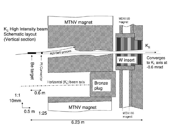
Figure 1: View of the 2002 modifications to the beam line.

Fig. 1 shows the modifications with respect to the previous ${K_{S}}$  beam line described in  [10]. The ${K_{L}}$  beam line was blocked and an additional sweeping magnet was installed to cover the defining section of the ${K_{S}}$  collimator. To reduce the number of photons in the neutral beam, primarily from $\pi^{0}$ decays, a platinum absorber 24 mm thick was placed in the beam between the target and a sweeping magnet, which deflected charged particles. A 5.1 m thick collimator, the axis of which formed an angle of 4.2 mrad to the proton beam direction, selected a beam of neutral long-lived particles (${{K_{S}}}$, ${{K_{L}}}$, $\Lambda^{0}$, $\Xi^{0}$, $n$ and $\gamma$). On average $2\times 10^{5}$ ${{K_{S}}}$ per spill decayed in the fiducial volume downstream of the collimator with a mean energy of 120 GeV.

2.2 Detector

The detector was designed for the measurement of $Re(\epsilon^{\prime}/\epsilon)$[10]. In order to minimize the interactions of the neutral beam with air, the collimator was immediately followed by a $\sim$ 90 m long evacuated tank which was terminated by a 0.3% $X_{0}$ thick Kevlar window. The detector was located downstream of this tank.

2.2.1 Tracking

The detector included a spectrometer housed in a helium gas volume with two drift chambers before and two after a dipole magnet with a horizontal transverse momentum kick of 265 MeV/c. Each chamber had four views (x, y, u, v), each of which had two sense wire planes. The resulting space points were typically reconstructed with a resolution of $\sim 150$ $\mu$m in each projection. The spectrometer momentum resolution could be parameterized as:

$$\sigma_{p}/p=0.48\%\oplus 0.015\%\times p$$

where $p$ is in GeV/c. This gave a resolution of 3 MeV/c² when reconstructing the kaon mass in ${{K_{S}}\rightarrow{\pi^{+}\pi^{-}}}$ decays. The track time resolution was $\sim~{}1.4$ ns.

2.2.2 Electromagnetic Calorimetry

The detection and measurement of the electromagnetic showers were achieved with a liquid krypton calorimeter (LKr), 27 radiation lengths deep, with a $\sim$ 2 cm $\times$ 2 cm cell cross-section.

The energy resolution, expressing $E$ in GeV, may be parameterized as [11]:

$$\sigma(E)/E=3.2\%/\sqrt{E}\oplus 9\%/E\oplus 0.42\%$$

The transverse position resolution for a single photon of energy larger than 20 GeV was better than 1.3 mm, and the corresponding mass resolution at the $\pi^{0}$ mass was $\sim$ 1 MeV/c². The time resolution of the calorimeter for a single shower was better than $\sim~{}300$ ps.

2.2.3 Scintillator Detectors

A scintillator hodoscope was located between the spectrometer and the calorimeter. It consisted of two planes, segmented in horizontal and vertical strips and arranged in four quadrants. Further downstream there was an iron-scintillator sandwich hadron calorimeter, followed by muon counters consisting of three planes of scintillator, each shielded by an iron wall. The fiducial volume of the experiment was principally determined by the LKr calorimeter acceptance, together with seven rings of scintillation counters used to veto activity outside this region.

2.2.4 Trigger and Readout

The detector was sampled every 25 ns with no dead time and the samples were recorded in a time window of $200$ ns encompassing the event trigger time. This allowed the rate of accidental activity to be investigated in appropriate time sidebands.

The event trigger for the signal ${{K_{S}}\rightarrow{\pi^{0}}e^{+}e^{-}}$ had both hardware and software parts:

• The hardware trigger [12] selected events satisfying the following conditions:

  • hit multiplicity in the first drift chamber compatible with one or more tracks;

  • hadron calorimeter energy less than 15 GeV;

  • electromagnetic calorimeter energy greater than 30 GeV;

  • the centre of energy of the electromagnetic clusters (see eq.  5 below) less than 15 cm from the beam axis;

  • the decay occurring within six $K_{S}$ lifetimes from the end of the collimator;

  • no hits in the two ring scintillator counters farthest downstream.

• The software trigger required:

  • at least two tracks in the drift chambers and two extra, well-separated clusters each with energy greater than 2 GeV;

  • the tracks projected from the drift chamber, after the magnet, had to match to clusters in the LKr within 5 cm;

  • the tracks had to be compatible with being electrons or positrons using the condition that the ratio $E/p$, between the cluster energy in the LKr, $E$, and the momentum measured with the drift chambers, $p$, had to be greater than 0.85.

  • a cluster separation of more than 5 cm was required to limit the degradation of the energy resolution due to energy sharing between closely spaced clusters.

The events that satisfied the trigger conditions were recorded and reprocessed with improved calibrations to obtain the final data sample.

2.3 Event selection

For the analysis of the data, signal and control regions were defined. These regions were masked while the cuts to reject the background were tuned using both data and Monte Carlo simulation.

The signal channel ${{K_{S}}\rightarrow{\pi^{0}}e^{+}e^{-}}$ required the identification of an electron and a positron accompanied by two additional clusters in the LKr.

Tracks reconstructed from the spectrometer which matched an LKr cluster were labelled as an electron or positron by requiring three conditions to be met: no more than 3 ns difference between track time and cluster time; $0.95<E/p<1.05$; and less than 2 cm between the projected track and the cluster coordinates in the LKr.

We define $\Delta t$ to be the difference between the average time of the two clusters associated with tracks and the average time of the two neutral clusters. Events were accepted if $|\Delta t|<3$ ns.

Events with extra tracks or extra clusters within 3 ns of the average time of the tracks or clusters and with an energy larger than 1.5 GeV were rejected. To minimize the effect of energy sharing on cluster reconstruction, a minimum cluster separation of 10 cm was imposed. In addition, a distance greater than 2 cm between the impact points of the two tracks at the first drift chamber was required.

Four quantities related to the decay vertex were computed.

• neutral vertex.

  The vertex position was computed from the energies and positions of the four clusters in the LKr according to

  $$z_{\text{\em neutral}}=z_{LKr}-\sqrt{\Sigma_{i,j>i}E_{i}E_{j}d_{ij}^{2}}/M_{K}$$ (4)

  where $z_{LKr}$ is the longitudinal position of the front face of the LKr; $M_{K}$ is the kaon mass, $E_{i,j}$ is the energy of the $(i,j)^{th}$ cluster and $d_{i,j}$ is the distance between clusters $i$ and $j$. In the case of the photons these are the $x,y$ shower positions in the LKr. For the $e^{\pm}$ tracks, in order to cancel the deflection due to the dipole magnet, the (x,y) positions were calculated by extrapolating the tracks from their positions in the first two drift chambers to the face of the LKr. The $x$ and $y$ coordinates of the neutral vertex were found by extrapolating the position of each track before the magnet to the position of $z_{\text{\em neutral}}$. The average of the two measurements was taken as the $(x,y)$ vertex position.

  The neutral vertex was used to compute the invariant mass of the two photons, ${m_{\gamma\gamma}}$.

• charged vertex.

  The position of the charged vertex can be calculated using the constraint that the kaon decay should lie on the straight line joining the target and the point defined as $(x_{cog},y_{cog})$:

  $$x_{cog}={{(\sum_{i}E_{i}x_{i})}}/{\sum_{i}E_{i}}~{}~{}~{}~{}y_{cog}={{(\sum_{i}E_{i}y_{i})}}/{\sum_{i}E_{i}}$$ (5)

  where $E_{i}$, $x_{i}$ and $y_{i}$ are the energy and positions of the $i$-th cluster.

  For each track, the closest distance of approach between this line and the track was found, giving two measurements which were then averaged to give the charged vertex position.

  The charged vertex was then used to compute ${m_{ee\gamma\gamma}}$, the invariant mass of the four decay products.

• $\pi^{0}$ vertex.

  The $\pi^{0}$ vertex position along the beam direction was computed in a similar way to the neutral vertex, but using only the two photon clusters and imposing the $\pi^{0}$ mass, $M_{\pi^{0}}$, instead of the kaon mass.

• track vertex.

  The track vertex is at the position of the closest distance of approach of the two tracks.

The $z$ position of the $\pi^{0}$ and track vertices had to be greater than 50 cm (one standard deviation) beyond the collimator exit in order to reject any interactions occurring in the collimator. Assuming the observed event to be a kaon decay, the proper lifetime was computed from the position of the neutral vertex, taking the end of the final collimator as the origin. A cut at 2.5 $K_{S}$ lifetimes was then applied. The kaon momentum was required to be between 40 and 240 GeV/c.

3 Signal and Control regions

The signal region was defined as :

• $|m_{\gamma\gamma}-M_{\pi^{0}}|<2.5\times\sigma_{{m_{\gamma\gamma}}}$

• $|{m_{ee\gamma\gamma}}-M_{K}|<2.5\times\sigma_{{m_{ee\gamma\gamma}}}$

To evaluate the resolutions, $\sigma_{{m_{ee\gamma\gamma}}}$ and $\sigma_{{m_{\gamma\gamma}}}$, we studied the channel ${{K_{S}}\rightarrow{\pi^{0}}{\pi_{D}^{0}}}$, for which we measured $\sigma_{{m_{ee\gamma\gamma\gamma}}}$ = 6.5 MeV/c² and $\sigma_{{m_{\gamma\gamma}}}$ = 1 MeV/c² respectively. These values were found to be in agreement with a Monte Carlo simulation based on GEANT [13]. For the decay ${{K_{S}}\rightarrow{\pi^{0}}e^{+}e^{-}}$, the Monte Carlo prediction of $\sigma_{{m_{ee\gamma\gamma}}}$ was 4.6 MeV/c² and this value was used in defining the signal region. The better resolution is due to the fact that the $e^{+}e^{-}$ opening angle is on average larger than for the decay ${{K_{S}}\rightarrow{\pi^{0}}{\pi_{D}^{0}}}$.

The ${m_{\gamma\gamma}}$ resolution, $\sigma_{{m_{\gamma\gamma}}}$, at the ${\pi^{0}}$ mass was found to be 1 MeV/c² in agreement with the Monte Carlo simulation.

A control region was also defined as:

• $3\times\sigma_{{m_{\gamma\gamma}}}<|{m_{\gamma\gamma}}-M_{\pi^{0}}|<6\times\sigma_{{m_{\gamma\gamma}}}$

• $3\times\sigma_{{m_{ee\gamma\gamma}}}<|{m_{ee\gamma\gamma}}-M_{K}|<6\times\sigma_{{m_{ee\gamma\gamma}}}$

Both the signal and the control regions were kept masked while cuts to reject the background were studied.

4 Background Rejection

A large number of possible background channels was studied. These channels were of two types:

• a single kaon or hyperon decay which reproduced an event falling into the ${{K_{S}}\rightarrow{\pi^{0}}e^{+}e^{-}}$ signal region

• fragments from two primary decays which happen to coincide in time and space and fall into the signal box.

The background contribution from the channels considered was reduced by imposing additional requirements.

A background source is from the decay ${{K_{S}}\rightarrow{\pi^{0}\pi^{0}}}$ where two photons from different $\pi^{0}$’s converted either internally (i.e. ${{K_{S}}\rightarrow{\pi_{D}^{0}}{\pi_{D}^{0}}}$) or externally and one electron and one positron from different $\pi^{0}$’s were outside the detector acceptance. In order to reject events from this source the invariant masses of the two electron-photon pairs, $m_{e^{+}\gamma_{1}}$,$m_{e^{-}\gamma_{2}}$ and $m_{e^{+}\gamma_{2}}$,$m_{e^{-}\gamma_{1}}$, were computed using the charged vertex position. A priori, the combination corresponding to electron-photon from the same $\pi^{0}$ has an invariant mass smaller than $M_{\pi^{0}}$. Thus events were rejected if both $m_{e\gamma}$ masses were measured to be smaller than $M_{\pi^{0}}+\delta$. The constant $\delta$ was chosen equal to 30 MeV/c², which corresponded to $\sim 10~{}\sigma_{m_{e\gamma}}$.

Another source of background was due to $\pi^{0}\pi^{0}$ decays where one or more photons from a single $\pi^{0}$ decay converted (either internally or externally). These decays are kinematically constrained to have $m_{e^{+}e^{-}}<M_{\pi^{0}}$ and in order to reject this background the analysis was restricted to the event sample with invariant mass $m_{e^{+}e^{-}}>M_{\pi^{0}}+\epsilon$. To determine $\epsilon$, we analysed the $m_{ee}$ distribution from data and compared it to a Monte Carlo simulation where the different components were identified. In fig. 2.a we show the $m_{ee}$ distribution for data (full dots) and superimposed the contributions from of all relevant background sources. Above the $\pi^{0}$ mass the tail of the $m_{ee}$ distribution falls rapidly to zero. The constant $\epsilon$ was also chosen equal to 30 MeV/c² and the analysis was therefore restricted to the region $m_{e^{+}e^{-}}>M_{\pi^{0}}+30$ MeV/c² = 165 MeV/c², where $\gamma$ conversions or decays from a single $\pi^{0}$ give a negligible contribution to the background. This was confirmed from the analysis of events with same sign-tracks. This sample contained events where both photons from a single $\pi^{0}$ converted and both the electrons or the positrons were in the acceptance. The $m_{e^{\pm}e^{\pm}}$ distribution is shown in fig. 2.b, where data and Monte Carlo are compared. No events with $m_{e^{\pm}e^{\pm}}>165$ MeV/c² were found.

To reject the background due to electron bremsstrahlung, the invariant mass of any $e\gamma$ combination was required to be larger than 20 MeV/c².

The background from $\Xi^{0}\rightarrow\Lambda\pi^{0}$ and $\Lambda\rightarrow p\pi^{-}$ decays was reduced to a negligible level by exploiting the large momentum asymmetry in both the $\Lambda\pi^{0}$ and the $p\pi^{-}$ final states. ${{K_{S}}\rightarrow{\pi^{0}}e^{+}e^{-}}$ candidates were required to have $(P_{\Lambda}-P_{\pi^{0}})/(P_{\Lambda}+P_{\pi^{0}})$ smaller than 0.4 or $(P_{p}-P_{\pi^{-}})/(P_{p}+P_{\pi^{-}})$ smaller than 0.5. A similar cut was used to remove ${\overline{\Xi^{0}}}$ and ${\overline{\Lambda}}$.

The possibility of proton and pion misidentification as $e^{\pm}$ was considered and final states which contained these particles were found to make a negligible contribution to the background after the application of the $E/p$ requirement.

5 Estimate of the Residual Background

After the selection outlined above three sources of background were found to be non-negligible:

• $K_{L,S}\rightarrow e^{+}e^{-}\gamma\gamma$

  The $e^{+}e^{-}\gamma\gamma$ component was measured using $K_{L}$ data from the 2001 run, in which the number of $K_{L}\rightarrow e^{+}e^{-}\gamma\gamma$ decays was $\sim$ 10 times the sum of the ${K_{L}}$ and $K_{S}\rightarrow e^{+}e^{-}\gamma\gamma$ expected in the present experiment. The distribution of ${m_{ee\gamma\gamma}}$ versus ${m_{\gamma\gamma}}$ for these events is shown in fig. 3. Using a linear extrapolation from the low ${m_{\gamma\gamma}}$ region to the signal region, the background from this channel was estimated to be $0.08^{+0.03}_{-0.02}$ events.

• ${{K_{S}}\rightarrow{\pi_{D}^{0}}{\pi_{D}^{0}}}$

  This was evaluated using full Monte Carlo simulation for a sample which was 30 times greater than the data, and the background was estimated to be less than 0.01 events in the signal region.

• Accidental backgrounds.

  This component was studied using data with the timing requirements relaxed. Events in the time sidebands, satisfying all the other cuts, were used to extrapolate the background from the control to the signal region. A further correction was applied to account for the background shape in the $m_{\gamma\gamma}$ versus $m_{e^{+}e^{-}\gamma\gamma}$ plane as predicted by a simulation.

  The contribution due to this component was $0.07^{+0.07}_{-0.03}$ events in the signal region.

Other sources of background were considered, for instance that due to resonances produced by a single proton in the target, and decaying to a pair of kaons or a $K\Lambda$ pair in the fiducial region. These contributions were found to be negligible.

With all the cuts applied, the control region was unmasked to estimate the final background contribution to the signal. No events were found in the control region, consistent with the background prediction of 0.33 events. Only one background event was found in a much larger region (corresponding to $17\times\sigma_{m_{K}}$ and $20\times\sigma_{m_{\gamma\gamma}}$). The background estimate is summarised in Table 1.

The resulting estimate of the total background in the signal region was $0.15^{+0.10}_{-0.04}$ events.

6 Normalisation.

The trigger efficiency was measured using a control sample of $\sim 8.6\times 10^{6}$ ${{K_{S}}\rightarrow{\pi^{0}}{\pi_{D}^{0}}}$ decays, which differed topologically from ${{K_{S}}\rightarrow{\pi^{0}}e^{+}e^{-}}$ only in having an extra photon. This sample was collected with the same trigger chain. The trigger efficiency, measured with a sample of triggers collected requiring minimal bias conditions, was found to be 99.0%. The acceptance, including the selection criteria, was found to be 3.3% for $\pi^{0}\pi^{0}_{D}$, evaluated using a Monte Carlo simulation. The Monte Carlo simulation was found to be in good agreement with the ${{K_{S}}\rightarrow{\pi^{0}}{\pi_{D}^{0}}}$ data. To obtain the ${{K_{S}}\rightarrow{\pi^{0}}e^{+}e^{-}}$ branching ratio, the $K_{S}$ flux was calculated using the channel ${{K_{S}}\rightarrow{\pi^{0}}{\pi_{D}^{0}}}$ for normalisation, which was selected using the same trigger. Using the value for the branching ratio $BR({{K_{S}}\rightarrow{\pi^{0}}{\pi_{D}^{0}}})=7.43\times 10^{-3}$ [14] the $K_{S}$ flux was calculated, for kaon energies between 40 and 240 GeV/c and kaon lifetimes between zero and 2.5 $K_{S}$ mean lifetimes from the collimator exit. The total number of ${K_{S}}$ decaying within the fiducial volume was $(3.51\pm 0.17)\times 10^{10}$.

7 Result

When the signal region was unmasked seven events were found (fig. 4). With an expected background of $0.15^{+0.10}_{-0.04}$ events, this corresponds to a signal of $6.85^{+3.8}_{-1.8}$. The probability that such a signal is consistent with background is $\sim 10^{-10}$. We therefore interpret the signal as the first observation of the ${{K_{S}}\rightarrow{\pi^{0}}e^{+}e^{-}}$ decays.

Fig. 5 shows the $m_{\gamma\gamma}$ and the $m_{e^{+}e^{-}\gamma\gamma}$ distributions of the events compared to the detector mass resolutions. In Table 2, some of the kinematical quantities for each event are summarised.

In order to calculate the ${{K_{S}}\rightarrow{\pi^{0}}e^{+}e^{-}}$ acceptance, the amplitude for the decay was needed. This was taken from the Chiral Perturbation Theory prediction given in [6], and is of the form:

$$A[K(k)\rightarrow\pi(p)e^{+}(p_{+})e^{-}(p_{-})]={\frac{-e^{2}}{{m_{\text{\em K}}}^{2}(4\pi)^{2}}}W(z)(k+p)^{\mu}{\bar{u}}_{l}(p_{-})\gamma_{\mu}v_{l}(p_{+})$$ (6)

where $k$, $p$, $p_{+}$ and $p_{-}$ are the four-momenta of the kaon, pion, positron and electron respectively; $m_{\text{\em K}}$ is the kaon mass; $W(z)$ is the electro-magnetic transition form factor, with $z=(k-p)^{2}/{m_{\text{\em K}}}^{2}$. As a consequence of gauge invariance, the form factor dependence on $z$ vanishes to lowest order and therefore can be represented as a polynomial. For $K_{S}$ decays, the form factor $W(z)$ was approximated to $W(z)\sim a+b\times z$ [6].

The $a$ and $b$ parameters have recently been measured for charged kaons, and the ratio $a/b$ found to be 1.12  [15].

The $m_{ee}$ distributions resulting from $W(z)=1$ and $W(z)=a+b\times z$ are shown in fig. 6.a.

The overall ${{K_{S}}\rightarrow{\pi^{0}}e^{+}e^{-}}$acceptance depends on the form factor. To remove this form factor dependence, an acceptance was calculated for each event using fig. 6.b, where the acceptance is given as a function of $m_{ee}$, using $W(z)=1$. The values are given in Table 2. The average geometrical acceptance of the 7 events is 0.15, while the average analysis efficiency is 0.44, which results in an average efficiency of $0.066\pm 0.004$.

From the ${{K_{S}}\rightarrow{\pi^{0}}{\pi_{D}^{0}}}$ flux and the signal of 6.85 events, the branching ratio for $m_{ee}>0.165$ GeV/c² was computed:

$BR({{K_{S}}\rightarrow{\pi^{0}}e^{+}e^{-}},\ m_{ee}>0.165$ GeV/c${}^{2})=(3.0^{+1.5}_{-1.2}(\text{stat})\pm 0.2(\text{syst}))\times 10^{-9}.$

The quoted uncertainties correspond to a 68.27% confidence level [16]. The systematic uncertainty includes the uncertainty of the flux measurement and of the acceptance.

8 Discussion

In Chiral Perturbation theory the $BR({{K_{S}}\rightarrow{\pi^{0}}e^{+}e^{-}})$ is related to the parameter $a_{S}$, which measures the strength of the indirect CP-violating term in ${{K_{L}}\rightarrow{\pi^{0}}e^{+}e^{-}}$decay as explained in [6] and eq. 1.

Using a vector matrix element with no form factor dependence, the measured branching ratio was extrapolated to the full $m_{ee}$ spectrum to obtain:

$$BR({{K_{S}}\rightarrow{\pi^{0}}e^{+}e^{-}})=(5.8^{+2.8}_{-2.3}(\text{stat})\pm 0.8(\text{syst}))\times 10^{-9}$$

The systematic error is dominated by the uncertainty in the extrapolation due to the form factor dependence.

It was then possible to extract the parameter $|a_{S}|$:

$$|a_{S}|=(1.06^{+0.26}_{-0.21}(\text{stat})\pm 0.07(\text{syst}))$$

The measurement of $a_{S}$ allows the branching ratio BR(${{K_{L}}\rightarrow{\pi^{0}}e^{+}e^{-}}$) to be predicted as a function of $Im(\lambda_{t})$ to within a sign ambiguity (see eq. 3). The effect of the sign ambiguity can be seen in fig. 7.a.

Alternatively, as shown in fig. 7.b, by using the global fit value for $Im(\lambda_{t})=(1.30\pm 0.12)\times 10^{-4}$ obtained from b-decay  [17], BR(${{K_{L}}\rightarrow{\pi^{0}}e^{+}e^{-}}$) can be expressed as function of $|a_{S}|$.

Using the measured value of $|a_{S}|$ and the global fit for $Im(\lambda_{t})$, eq. 3 reduces to:

$${\rm BR}({{K_{L}}\rightarrow{\pi^{0}}e^{+}e^{-}})_{\text{CPV}}\simeq(17.2_{\text{indirect}}\pm 9.4_{\text{interference}}+4.7_{\text{direct}})\times 10^{-12}.$$

The CP conserving component can be obtained from the study of the ${{K_{L}}\rightarrow{\pi^{0}}\gamma\gamma}$ decay. A measurement made by the KTeV collaboration  [18] found $BR({{K_{L}}\rightarrow{\pi^{0}}e^{+}e^{-}})_{CPC}=(1-2)\times 10^{-12}$. A more recent measurement quoted $BR({{K_{L}}\rightarrow{\pi^{0}}e^{+}e^{-}})_{CPC}=0.47^{+0.22}_{-0.18}\times 10^{-12}$ [19] suggesting that the CP-conserving component is negligible.

Given the measured value of $a_{S}$ the direct CP violated component predicted from the Standard Model is small with respect to the indirect component. If the sign of $a_{S}$ turns out to be negative then BR(${{K_{L}}\rightarrow{\pi^{0}}e^{+}e^{-}}$) retains some sensitivity to ${\rm Im}(\lambda_{t})$ through the interference term.

Source	control region	signal region
${{K_{S}}\rightarrow{\pi_{D}^{0}}{\pi_{D}^{0}}}$	0.03	$<0.01$
${{K_{L}}\rightarrow ee\gamma\gamma}$	0.11	0.08
Accidentals	0.19	0.07
Total background	0.33	0.15

Table 1: Summary of the background estimate.

Event no.	$K_{S}$ momentum	$\tau/\tau_{S}$	$m_{ee}$	Acceptance
	GeV/c		GeV/c2
1	84.6	0.74	0.291	0.058
2	128.2	0.50	0.267	0.066
3	114.1	1.02	0.173	0.084
4	83.9	2.09	0.272	0.066
5	130.8	1.46	0.303	0.052
6	121.2	1.49	0.298	0.058
7	94.2	1.64	0.253	0.075

Table 2: Kinematical quantities of the seven events found in the signal region.

      

Figure 2: Distributions of $m_{ee}$ after all the cuts have been applied. Superimposed we show the Monte Carlo predictions from all important sources. Figure a) shows the components with opposite-sign tracks; figure b) shows the ones with same-sign tracks.

Figure 3: Scatter plot of ${m_{ee\gamma\gamma}}$ versus $m_{\gamma\gamma}$ for events selected as $K_{L}\rightarrow e^{+}e^{-}\gamma\gamma$ in the 2001 data. The boxes are representing the $3\sigma$ and $6\sigma$ regions.

      

Figure 4: Scatter plot of ${m_{ee\gamma\gamma}}$ versus $m_{ee}$(a) and ${m_{ee\gamma\gamma}}$ versus $m_{\gamma\gamma}$ (b) for events passing all the cuts described in the text. The regions of $3\sigma$ and $6\sigma$ are shown.

      

Figure 5: $m_{\gamma\gamma}$ (a) and ${m_{ee\gamma\gamma}}$ distributions (b) for the 7 events found in the signal region. The expected Gaussian mass resolutions are superimposed (solid line).

      

Figure 6: $m_{ee}$ distributions from Monte Carlo, with and without the form factor (a); acceptance as a function of $m_{ee}$ (b).

      

Figure 7: Branching fraction of ${{K_{L}}\rightarrow{\pi^{0}}e^{+}e^{-}}$as a function of $Im(\lambda_{t})$ (a), and as a function of the parameter $a_{S}$ (b).

References

- [1] L. M. Sehgal, Nuclear Physics B19 (1970) 445.
- [2] G. Ecker, A. Pich, and E. de Rafael, Nuclear Physics B291 (1987) 692.
- [3] C. Bruno and J. Prades, Zeitschrift für Physik C57 (1993) 585.
- [4] G. Ecker, A. Pich and E. de Rafael, Nuclear Physics B303 (1988) 665.
- [5] J.F. Donoghue, F. Gabbiani, Physical Review D51 (1995) 2187.
- [6] G. D’Ambrosio, G. Ecker, G. Isidori, and J. Portoles, Journal of High Energy Physics 08 (1998) 004.
- [7] A. Alavi-Harati et al., Physical Review Letters 86 (2001) 397.
- [8] A. Lai et al., Physics Letters B514 (2001) 253.
- [9] G. Isidori, International Journal of Modern Physics A17 (2002) 3078.
- [10] J.R. Batley et al., Physics Letters B544 (2002) 97.
- [11] G. Unal, NA48 Collaboration, in: IX International Conference on Calorimetry, October 2000, Annecy, France, hep-ex/0012011.
- [12] G. Barr et al., Nuclear Instruments and Methods in Physics Research A485 (2002) 676.
- [13] GEANT Detector Description and Simulation Tool, CERN Program Library Long Write-up W5013 (1994).
- [14] K. Hagiwara et al., Physical Review D 66 (2000) 1.
- [15] R. Appel et al., Physical Review Letters 83 (1999) 4482.
- [16] G.J. Feldman and R.D. Cousins, Physics Review D57 (1998) 3873.
- [17] S. H. Kettell, L. G. Landsberg, and H. Nguyen, hep-ph/0212321.
- [18] A. Alavi-Harati et al., Physical Review Letters 83 (1999) 917.
- [19] A. Lai, et al., Physics Letters B536 (2002) 229.