The BABAR Collaboration

We present a preliminary measurement of the time-dependent $C\!P$ asymmetries in decays of neutral $B$ mesons to the final states $D^{*\mp}\pi^{\pm}$, using approximately $82$ million $B\kern 1.79993pt\overline{\kern-1.79993ptB}{}$ events collected by the BABAR experiment at the PEP-II storage ring. Events containing these decays are selected with a partial reconstruction technique, in which only the high momentum $\pi^{\pm}$ and the low momentum pion from the $D^{*\mp}$ decay are reconstructed. The flavor of the other $B$ meson in the event is tagged using the information from kaon and lepton candidates. We measure the time-dependent $C\!P$ asymmetry ${\cal A}=-0.063\pm 0.024~{}(stat.)\pm 0.017~{}(syst.)$. We interpret these results in terms of the angles of the unitarity triangle to set a bound on $|\sin(2\beta+\gamma)|$.

Contribution to the International Europhysics Conference On High-Energy Physics (HEP 2003), 7/17—7/23/2003, Aachen, Germany

1 INTRODUCTION

Measuring the angles of the Cabibbo-Kobayashi-Maskawa (CKM) unitarity triangle [1] will allow us to overconstrain this triangle and to test the Standard Model interpretation of $C\!P$ violation in the quark sector. A crucial step in this scientific program is the measurement of the angle $\gamma=\arg{\left(-V_{ud}V_{ub}^{\ast}/V_{cd}V_{cb}^{\ast}\right)}$ of the unitarity triangle.

The neutral $B$ meson decay modes $B^{0}\rightarrow{D^{*}}^{\pm}h^{\mp}$, where $h$ is a light hadron ($\pi,\rho,a_{1}$), have been proposed for use in measurements of $\sin(2\beta+\gamma)$ [2], where $\beta=\arg{\left(-V_{cd}V_{cb}^{\ast}/V_{td}V_{tb}^{\ast}\right)}$. Since the time-dependent $C\!P$ asymmetries in these modes are expected to be of order 2%, large data samples and multiple decay channels are required for a statistically significant measurement. The technique of partial reconstruction of $D^{*-}$ mesons, in which only the soft (low momentum) pion $\pi_{s}$ from the decays $D^{*-}\rightarrow\kern 1.99997pt\overline{\kern-1.99997ptD}{}^{0}\pi_{s}^{-}$ or $D^{*+}\rightarrow D^{0}\pi_{s}^{+}$ is reconstructed, has already been used to select large samples of $B$ meson candidates [3].

This paper reports the preliminary results of a study of $C\!P$-violating asymmetries in $B^{0}\rightarrow D^{*\mp}\pi^{\pm}$ decays using the partial reconstruction technique. The analysis procedures for the selection of the signal and the reconstruction of the decay-time difference between the two $B$ mesons in the event are essentially the same as those we have already applied to the measurement of the $B^{0}$ lifetime [4].

2 PRINCIPLE OF THE MEASUREMENT

The decays $B^{0}\rightarrow D^{*\mp}\pi^{\pm}$ may proceed via a $b\rightarrow c\bar{u}d$ or a $b\rightarrow u\bar{c}d$ amplitude (see Figs. 2 and 2). Interference between these amplitudes through $B^{0}-\kern 1.79993pt\overline{\kern-1.79993ptB}{}^{0}$ mixing produces time-dependent $C\!P$-violation observables [2]. The probability that a state produced at time 0 as a $B^{0}$ or $\kern 1.79993pt\overline{\kern-1.79993ptB}{}^{0}$ decays into the final state $D^{*\mp}\pi^{\pm}$ at time $t$ is

$$P(B^{0}\rightarrow D^{*\mp}\pi^{\pm})(t)={1\over 4\tau}e^{-|t|/\tau}\left[1\pm C\cos(\Delta m_{d}t)+S^{\mp}\sin(\Delta m_{d}t)\right],$$ (1)

$$P(\kern 1.79993pt\overline{\kern-1.79993ptB}{}^{0}\rightarrow D^{*\mp}\pi^{\pm})(t)={1\over 4\tau}e^{-|t|/\tau}\left[1\mp C\cos(\Delta m_{d}t)-S^{\mp}\sin(\Delta m_{d}t)\right],$$ (2)

where $\tau$ is the $B^{0}$ lifetime, $\Delta m_{d}$ is the $B^{0}-\kern 1.79993pt\overline{\kern-1.79993ptB}{}^{0}$ mixing frequency, and we have defined

$$C = {1-r^{2}\over 1+r^{2}}\,,$$

$$S^{\pm} = {2r\over 1+r^{2}}\,\sin(2\beta+\gamma\pm\delta).$$ (3)

Here $\delta$ is an unknown $C\!P$-conserving phase , and $r$ is the ratio of the magnitudes of the $b\rightarrow u\bar{c}d$ and $b\rightarrow c\bar{u}d$ amplitudes

$$r=\frac{|A(\kern 1.79993pt\overline{\kern-1.79993ptB}{}^{0}\rightarrow D^{*-}\pi^{+})|}{|A(\kern 1.79993pt\overline{\kern-1.79993ptB}{}^{0}\rightarrow D^{*+}\pi^{-})|}.$$ (4)

Since the $b\rightarrow u\bar{c}d$ amplitude is doubly Cabibbo-suppressed with respect to the $b\rightarrow c\bar{u}d$ amplitude, one expects $r\approx 2\%$. Due to the small value of $r$, we use the approximations

$$C \approx 1,$$

$$S^{\pm} \approx 2r\sin(2\beta+\gamma\pm\delta).$$ (5)

In principle, $r$ can be measured from the first two terms in the square brackets of Eqs. 1 and 2. In practice, this requires sensitivity to terms of order $r^{2}$, which is not available with the statistics of current data sets.

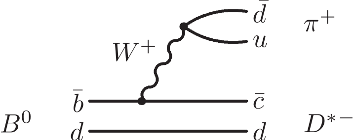
Figure 1: Feynman diagram for the Cabibbo-favored decay $B^{0}\rightarrow D^{*-}\pi^{+}$.

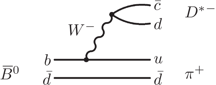
Figure 2: Feynman diagram for the Cabibbo-suppressed decay $\kern 1.79993pt\overline{\kern-1.79993ptB}{}^{0}\rightarrow D^{*-}\pi^{+}$.

Due to the small value of $r$, a large number of signal events is required in order to observe and measure the small time-dependent $C\!P$ asymmetry. In the partial reconstruction method, the decay $B^{0}\rightarrow D^{*\mp}\pi^{\pm}$ is identified by reconstructing only the hard (high momentum) $\pi^{\pm}$ and the soft pion $\pi_{s}^{\mp}$ from the decay of the $D^{*\mp}$. The four-momentum of the unreconstructed neutral $D$ meson produced in the ${D^{*}}^{\mp}$ decay is calculated from the two observed tracks and the kinematic constraints relevant for signal decays. Partial reconstruction provides a way to obtain very large single-mode signal samples, by making use of events that cannot be fully reconstructed.

3 THE BABAR DETECTOR AND DATASET

The data used in this analysis were collected with the BABAR detector at the PEP-II storage ring. The data sample consists of 76.4 fb^-1 collected on the $\mathchar 28935\relax(4{\rm S})$ resonance, and 7.6 fb^-1 collected at an $e^{+}e^{-}$ center-of-mass (CM) energy approximately 40 $\mathrm{\,Me\kern-1.00006ptV}$ below the resonance peak. Samples of simulated events with an equivalent luminosity four times larger than the data were analyzed through the same analysis chain.

The BABAR detector is described in detail elsewhere [6]. We provide a brief description of the main components and their use in this analysis. Charged particle trajectories are measured by a combination of a five-layer silicon vertex tracker (SVT) and a 40-layer drift chamber (DCH) in a 1.5-T solenoidal magnetic field. Tracks with low transverse momentum can be reconstructed in the SVT alone, thus extending the charged-particle detection down to transverse momenta of $\sim 50$${\mathrm{\,Me\kern-1.00006ptV\!/}c}$. Photons and electrons are detected in a CsI(Tl) electromagnetic calorimeter (EMC), with photon energy resolution $\sigma_{E}/E=0.023(E/\mathrm{\,Ge\kern-1.00006ptV})^{-1/4}\oplus 0.019$. A ring-imaging Cherenkov detector (DIRC) is used for charged particle identification, augmented by energy loss information from the SVT and DCH. The instrumented flux return (IFR) is equipped with resistive plate chambers to identify muons.

4 ANALYSIS METHOD

4.1 Partial Reconstruction of $B^{0}\rightarrow D^{*\mp}\pi^{\pm}$

In the partial reconstruction of a $B^{0}\rightarrow D^{*\mp}\pi^{\pm}$ candidate, only the hard pion track from the $B$ decay and the soft pion track $\pi_{s}$ from the decays $D^{*-}\rightarrow\kern 1.99997pt\overline{\kern-1.99997ptD}{}^{0}\pi_{s}^{-}$ or $D^{*+}\rightarrow D^{0}\pi_{s}^{+}$ are reconstructed. The cosine of the angle between the momenta of the $B$ and the hard pion in the CM frame is then computed:

$$\cos\theta_{Bh}={M_{{D^{*}}^{-}}^{2}-M_{B^{0}}^{2}-M_{\pi}^{2}+E_{\rm CM}E_{h}\over 2p_{B}|\vec{p}_{h}|},$$ (6)

where $M_{x}$ is the nominal mass of particle $x$ [7], $E_{h}$ and $\vec{p}_{h}$ are the measured CM energy and momentum of the hard pion, $E_{\rm CM}$ is the total CM energy of the beams, and $p_{B}=\sqrt{E_{\rm CM}^{2}/4-M_{B^{0}}^{2}}$. Events are required to be in the physical region $|\cos\theta_{Bh}|<1$. Given $\cos\theta_{Bh}$ and the measured momenta of the $\pi_{h}$ and $\pi_{s}$, the $B$ four-momentum can be calculated up to an unknown azimuthal angle $\phi$ around ${\vec{p}}_{h}$. For every value of $\phi$, the expected $D$ four-momentum ${\cal P}_{D}(\phi)$ is determined from four-momentum conservation, and the corresponding $\phi$-dependent invariant mass $m(\phi)\equiv\sqrt{|{\cal P}_{D}(\phi)|^{2}}$ is calculated. We define the missing mass $m_{\rm miss}\equiv{1\over 2}\left[m_{\rm max}+m_{\rm min}\right]$, where $m_{\rm max}$ and $m_{\rm min}$ are the maximum and minimum values that $m(\phi)$ may obtain. In signal events, $m_{\rm miss}$ peaks at the nominal $D^{0}$ mass $M_{D^{0}}$, with a spread of about 3 ${\mathrm{\,Me\kern-1.00006ptV\!/}c^{2}}$. The distribution for combinatoric background events is significantly broader, making the missing mass the primary variable for distinguishing signal from background, as described below. We use four-momentum conservation to calculate the CM $D$ momentum vector with the arbitrary choice $\phi=0$, and use this variable as described below.

4.2 Backgrounds

In addition to $B^{0}\rightarrow D^{*\mp}\pi^{\pm}$ events, the above procedure yields a sample containing the following kinds of events: $B\rightarrow D^{*\mp}\rho^{\pm}$; peaking $B\kern 1.79993pt\overline{\kern-1.79993ptB}{}$ background (other than $B\rightarrow D^{*\mp}\rho^{\pm}$), defined as pairs of tracks coming from the same $B$ meson, with the soft pion originating from the decay of a charged $D^{*}$, including contributions from $B\rightarrow D^{**}\pi$ as well as non-resonant $B\rightarrow D^{*}\pi\pi$ decays; combinatoric $B$ background, defined as all remaining $B\kern 1.79993pt\overline{\kern-1.79993ptB}{}$ background events; continuum $e^{+}e^{-}\rightarrow q\overline{q}$, where $q$ represents a $u$, $d$, $s$, or $c$ quark.

4.3 Event Selection

To suppress the continuum background, we select events in which the ratio of the 2nd to the 0th Fox-Wolfram moment [8], computed using all charged particles and EMC clusters not matched to tracks, is smaller than 0.40. Hard pion candidates are required to be reconstructed with at least twelve DCH hits. Kaons and leptons are rejected based on information from the IFR, DIRC, energy loss in the SVT and DCH, or the ratio of the candidate’s EMC energy deposition to its momentum ($E/p)$. We define the $D^{*}$ helicity angle $\theta_{D^{*}}$ to be the angle between the flight directions of the $D$ and the $B$ in the $D^{*}$ rest frame, calculated with $\phi=0$. Taking advantage of the longitudinal polarization in signal events, we suppress background by requiring $|\cos\theta_{D^{*}}|$ to be larger than 0.4. All candidates are required to be in the range $1.81<m_{\rm miss}<1.88$ ${\mathrm{\,Ge\kern-1.00006ptV\!/}c^{2}}$. When multiple candidates are found in the same event, only the one with the $m_{\rm miss}$ value closest to $M_{D^{0}}$ is used.

4.4 Fisher Discriminant

To further discriminate against continuum events, we combine fifteen event shape variables into a Fisher discriminant [9] $F$. Discrimination is provided due to the fact that $q\overline{q}$ events tend to be jet-like, whereas $B\kern 1.79993pt\overline{\kern-1.79993ptB}{}$ events have a more spherical energy distribution. Rather than applying requirements to the variable $F$, we maximize efficiency by using it in the fits described below. The fifteen variables are calculated using two sets of particles. Set 1 includes all tracks and EMC clusters, excluding the hard and soft pion candidates; Set 2 is composed of Set 1, excluding all tracks and clusters with CM momentum within 1.25 rad of the CM momentum of the $D$, calculated with $\phi=0$. The variables, all calculated in the CM frame, are 1) the scalar sum of the momenta of all Set 1 tracks and EMC clusters in nine $20^{0}$ angular bins centered about the hard pion direction; 2) the value of the sphericity, computed with Set 1; 3) the angle with respect to the hard pion of the sphericity axis, computed with Set 2; 4) the direction of the particle of highest energy in Set 2 with respect to the hard pion; 5) the absolute value of the vector sum of the momenta of all the particles in Set 2 ; 6) the momentum $\vec{p}_{h}$ of the hard pion and its polar angle.

4.5 Decay Time Measurement and Flavor Tagging

We define $z_{\rm rec}$ to be the decay position along the beam axis of the partially reconstructed $B$ candidate. To find $z_{\rm rec}$, we fit the hard pion track with a beam spot constraint in the plane perpendicular to the beams, the $(x,y)$ plane. The actual vertical beam spot size is approximately $5~{}\mu$m, but the constraint is taken to be $30~{}\mu$m in the fit in order to account for the $B$ flight distance in the $(x,y)$ plane. The soft pion is not used in the fit, since it undergoes significant multiple scattering.

The decay position $z_{\rm tag}$ of the other $B$ in the event (the tag $B$) along the beam axis is obtained from all other tracks in the event, excluding all tracks whose CM momentum is within 1 rad of the $D$ CM momentum. The remaining tracks are fit with a beamspot constraint in the $(x,y)$ plane. The track with the largest contribution to the $\chi^{2}$ of the vertex, if greater than 6, is removed from the vertex, and the fit is carried out again, until no track fails this requirement.

We then calculate the decay distance $\Delta z=z_{\rm rec}-z_{\rm tag}$, and the decay-time difference $\Delta t=\Delta z/(\gamma\beta c)$. The machine boost parameter $\gamma\beta$ is calculated from the beam energies, and its average value over the run period is 0.55. The vertex fits used to determine $z_{\rm rec}$ and $z_{\rm tag}$ also yield the $\Delta z$ error $\sigma_{\Delta z}$ which is used to compute the event-by-event $\Delta t$ error $\sigma_{\Delta t}$.

The flavor of the tag $B$ is determined from lepton and kaon candidates. The lepton CM momentum is required to be greater than 1.1 ${\mathrm{\,Ge\kern-1.00006ptV\!/}c}$ in order to suppress “cascade” leptons originating in charm decays. We identify electron candidates using $E/p$, and the Cherenkov angle and number of photons detected in the DIRC. Muons are identified by the depth of penetration in the IFR. Kaons are identified using the ionization measured in the SVT and DCH, and the Cherenkov angle and number of photons detected in the DIRC. In either the lepton or kaon tagging category, if several tagging tracks are present, the track used for tagging is the one with the largest value of $\theta_{tag}$, the CM-frame angle between the track momentum and the $D$ momentum. This is done in order to minimize the impact of tracks originating from the unreconstructed $D$. If there are both identified leptons and kaons in the event, the event is tagged using the lepton tracks only.

We apply the following criteria in order to obtain good $\Delta t$ resolution: the $\chi^{2}$ probability of the $z_{\rm rec}$ vertex fit must be greater than 0.001; at least two tracks must be used for the tag $B$ vertex fit; $\sigma_{\Delta t}$ is required to be less than 2 ps; and $|\Delta t|$ is required to be less than 15 ps. To minimize the impact of tracks coming from the unreconstructed $D$, only tagging leptons (kaons) satifying $\cos\theta_{tag}<0.75$ ($\cos\theta_{tag}<0.50$) are retained.

4.6 Probability Density Function

The analysis is carried out with a series of unbinned maximum likelihood fits performed independently for the lepton-tagged and kaon-tagged events. The probability density function (PDF) is a function of the missing mass $m_{\rm miss}$, the Fisher discriminant $F$, the decay time difference $\Delta t$, and its error $\sigma_{\Delta t}$.

The PDF for on-resonance data is a sum over the PDFs of the identified event types,

$$\begin{array}[]{lllll}P=f_{B\kern 1.25995pt\overline{\kern-1.25995ptB}{}}\,\Bigl{\{}&&\kern-19.91684ptf_{\rho+\pi}\,(f_{D^{*}\pi}\,P_{D^{*}\pi}&&\kern-19.91684pt+(1-f_{D^{*}\pi})P_{D^{*}\rho})\\ &&\kern-19.91684pt+(1-f_{\rho+\pi})\Bigl{[}&&\kern-19.91684pt{\kern-11.38092pt}f_{\rm comb}\,P_{\rm comb}+(1-f_{\rm comb})P_{\rm peak}\Bigr{]}\Bigr{\}}+(1-f_{B\kern 1.25995pt\overline{\kern-1.25995ptB}{}})P_{q\overline{q}},\end{array}$$ (7)

where $P_{i}$ is the PDF for events of type $i$, and $f_{j}$ are relative fractions of events, each limited to lie in the range $[0,1]$. Each of the PDFs $P_{i}$ is a product of the form

$$P_{i}(m_{\rm miss},F,\Delta t,\sigma_{\Delta t},s_{\rm tag},s_{\rm mix})={\cal M}_{i}(m_{\rm miss})\,{\cal F}_{i}(F)\,T^{\prime}_{i}(\Delta t,\sigma_{\Delta t},s_{\rm tag},s_{\rm mix}),$$ (8)

where the variables $s_{\rm tag}$ and $s_{\rm mix}$ are determined by the flavor of the tag $B$ and the charge of the hard pion

$$s_{\rm tag} = \left\{\begin{array}[]{ll}+1,&\mathrm{tag\ }B=B^{0}\\ -1,&\mathrm{tag\ }B=\kern 1.79993pt\overline{\kern-1.79993ptB}{}^{0}\end{array}\right.,$$ (11)

$$s_{\rm mix} = \left\{\begin{array}[]{ll}+1,&\mathrm{unmixed}\\ -1,&\mathrm{mixed}\end{array}\right.,$$ (14)

and an event is labeled “unmixed” if the hard pion is a $\pi^{-}(\pi^{+})$ and the tag $B$ is tagged as a $B^{0}(\kern 1.79993pt\overline{\kern-1.79993ptB}{}^{0})$ and “mixed” otherwise. The functions ${\cal M}_{i}$, ${\cal F}_{i}$, and $T^{\prime}_{i}$ are described below. The parameters of $P_{i}$ are different for each event type, except where indicated otherwise.

The $m_{\rm miss}$ PDF for each event type $i$ is the sum of a bifurcated Gaussian plus an ARGUS function:

$${\cal M}_{i}(m_{\rm miss})=f^{\hat{\cal G}}_{i}\,\hat{\cal G}_{i}(m_{\rm miss})+(1-f^{\hat{\cal G}}_{i}){\cal A}_{i}(m_{\rm miss}),$$ (15)

where $f^{\hat{\cal G}}_{i}$ is the bifurcated Gaussian fraction. The functions $\hat{\cal G}_{i}$ and ${\cal A}_{i}$ are

$$\hat{\cal G}_{i}(x) \propto \biggl{\{}\matrix{\exp\left[-(x-M_{i})^{2}/2\sigma_{Li}^{2}\right],&x<M_{i}\cr\exp\left[-(x-M_{i})^{2}/2\sigma_{Ri}^{2}\right],&x>M_{i}},$$ (16)

$${\cal A}(x) \propto x\sqrt{1-\left({x/M^{A}_{i}}\right)^{2}}\;\exp\left[\epsilon_{i}\left(1-\left({x/M^{A}_{i}}\right)^{2}\right)\right]\,\Theta(M^{A}_{i}-x),$$ (17)

where $M_{i}$ is the peak of the bifurcated Gaussian, $\sigma_{Li}$ and $\sigma_{Ri}$ are its left and right widths, $\epsilon_{i}$ is the ARGUS exponent, $M^{A}_{i}$ is its end point, and the proportionality constants are such that each of these functions is normalized to unit area.

The Fisher discriminant PDF ${\cal F}_{i}$ for each event type is a bifurcated Gaussian, as in Eq. 16. The parameter values of ${\cal F}_{D^{*}\pi}$, ${\cal F}_{D^{*}\rho}$, ${\cal F}_{\rm peak}$, and ${\cal F}_{\rm comb}$ are identical.

The $\Delta t$-dependent part of the PDF for events of type $i$ is a convolution of the form

$$T^{\prime}_{i}(\Delta t,\sigma_{\Delta t},s_{\rm tag},s_{\rm mix})=\int d\Delta t_{\rm true}\;T_{i}(\Delta t_{\rm true},s_{\rm tag},s_{\rm mix})\,{\cal R}_{i}(\Delta t-\Delta t_{\rm true},\sigma_{\Delta t}),$$ (18)

where $T_{i}$ is the distribution of the true decay-time difference $\Delta t_{\rm true}$ and ${\cal R}_{i}$ is a resolution function that accounts for detector resolution and effects such as systematic offsets in the measured positions of vertices. The resolution function for events of type $i$ is the sum of three Gaussians:

$${\cal R}_{i}(\Delta t-\Delta t_{\rm true},\sigma_{\Delta t})=f^{n}_{i}\,{\cal G}^{n}_{i}(t_{r},\sigma_{\Delta t})+(1-f^{n}_{i}-f^{o}_{i})\,{\cal G}^{w}_{i}(t_{r},\sigma_{\Delta t})+f^{o}_{i}\,{\cal G}^{o}_{i}(t_{r},\sigma_{\Delta t}),$$ (19)

where $t_{r}$ is the residual $\Delta t-\Delta t_{\rm true}$, and ${\cal G}^{n}_{i}$, ${\cal G}^{w}_{i}$, and ${\cal G}^{o}_{i}$ are the “narrow”, “wide”, and “outlier” Gaussians. The narrow and wide Gaussians have the form

$${\cal G}^{j}_{i}(t_{r},\sigma_{\Delta t})\equiv{1\over\sqrt{2\pi}\,s^{j}_{i}\,\sigma_{\Delta t}}\exp\left(-\,{\left(t_{r}-b^{j}_{i}\sigma_{\Delta t}\right)^{2}\over 2(s^{j}_{i}\,\sigma_{\Delta t})^{2}}\right),$$ (20)

where the index $j$ takes the values $j=n,w$ for the narrow and wide Gaussians, and $b^{j}_{i}$ and $s^{j}_{i}$ are parameters determined by fits, as described in Sec. 5. The outlier Gaussian has the form

$${\cal G}^{o}_{i}(t_{r},\sigma_{\Delta t})\equiv{1\over\sqrt{2\pi}\,s^{o}_{i}}\exp\left(-\,{\left(t_{r}-b^{o}_{i}\right)^{2}\over 2(s^{o}_{i})^{2}}\right),$$ (21)

where in all fits the values of $b^{o}_{i}$ and $s^{o}_{i}$ are fixed to 0 ps and 8 ${\rm\,ps}$, respectively, and are later varied to evaluate systematic errors.

The PDF $T_{D^{*}\pi}(\Delta t_{\rm true},s_{\rm tag},s_{\rm mix})$ for signal events corresponds to Eqs. 1 and 2 with Eq. 5 and additional parameters to account for imperfect flavor tagging. We define $\omega_{B^{0}}$ ($\omega_{\kern 1.25995pt\overline{\kern-1.25995ptB}{}^{0}}$) to be the mistag probability of signal events whose tag $B$ was tagged as a $B^{0}$ ($\kern 1.79993pt\overline{\kern-1.79993ptB}{}^{0}$), when the tagging track is a daughter of the tag $B$. Then $\omega=(\omega_{B^{0}}+\omega_{\kern 1.25995pt\overline{\kern-1.25995ptB}{}^{0}})/2$ is the average mistag rate, and $\Delta\omega=\omega_{B^{0}}-\omega_{\kern 1.25995pt\overline{\kern-1.25995ptB}{}^{0}}$ is the mistag rate difference. We further define $\alpha$ to be the probability that the tagging lepton or kaon is a daughter of the unreconstructed $D$ produced in the $B^{0}\rightarrow D^{*\mp}\pi^{\pm}$ decay, and $\rho$ to be the probability that this track results in a mixed flavor tag. With these definitions, the signal PDF is written as

$$T_{D^{*}\pi}(\Delta t_{\rm true},s_{\rm tag},s_{\rm mix}) = \frac{1}{4\,\tau}\,e^{-\frac{|\Delta t_{\rm true}|}{\tau}}\times$$ (22)

$$\left\{(1-\alpha)\left[\left(1-s_{\rm tag}\,\Delta\omega\right)\right.\right.$$

$$+s_{\rm mix}\,(1-2\,\omega)\cos(\Delta m\Delta t_{\rm true})$$

$$\left.-s_{\rm tag}\,(1-2\,\omega)\,S^{\pm}\,\sin(\Delta m\Delta t_{\rm true})\right]$$

$$\left.+\alpha(1+s_{\rm mix}(1-2\rho))\right\},$$

where the value $\pm$ in $S^{\pm}$ is determined by the sign of the product ${s_{\rm tag}s_{\rm mix}}$. The last term accounts for the tags due to daughters of the unreconstructed $D$. The parameters $\tau$, $\Delta\omega$, $\omega$, $\Delta m$, and $S^{\pm}$ are determined from a fit to the data, as described below.

The tag $B$ may undergo a $b\rightarrow u\bar{c}d$ decay, and the kaon produced in the subsequent decay of the charmed meson may be used for tagging. This introduces additional terms, which are not present in Eq. 22. To take this effect into account, we use an alternative parameterization [10] for the kaon tags. In this parameterization [10], the coefficient of the $\sin(\Delta m\Delta t_{\rm true})$ term in Eq. 22 changes, to give

$$T_{D^{*}\pi}(\Delta t_{\rm true},s_{\rm tag},s_{\rm mix}) = \frac{1}{4\,\tau}\,e^{-\frac{|\Delta t_{\rm true}|}{\tau}}\times$$ (23)

$$\left\{(1-\alpha)\left[\left(1-s_{\rm tag}\,\Delta\omega\right)\right.\right.,$$

$$+s_{\rm mix}\,(1-2\,\omega)\,\cos(\Delta m\Delta t_{\rm true})$$

$$\left.-\left((1-2\,\omega)\,(s_{\rm tag}a+s_{\rm mix}c)+s_{\rm tag}s_{\rm mix}b(1-s_{\rm tag}\Delta\omega)\right)\sin(\Delta m\Delta t_{\rm true})\right]$$

$$\left.+\alpha(1+s_{\rm mix}(1-2\rho))\right\},$$

where

$$a \equiv 2r\sin(2\beta+\gamma)\cos\delta,$$ (24)

$$b \equiv 2r^{\prime}\sin(2\beta+\gamma)\cos\delta^{\prime},$$ (25)

$$c \equiv 2\cos(2\beta+\gamma)(r\sin\delta-r^{\prime}\sin\delta^{\prime}).$$ (26)

Here $r^{\prime}$ describes the effective ratio between the magnitudes of the $b\rightarrow u\overline{c}d$ and $b\rightarrow c\overline{u}d$ amplitudes in the tag side decays, and $\delta^{\prime}$ is the effective strong phase difference between these amplitudes. This parameterization neglects terms of order $r^{2}$ and $r^{\prime 2}$.

We take the $\Delta t$ PDF parameters of $B\rightarrow D^{*\mp}\rho^{\pm}$ events to be identical to those of the $B^{0}\rightarrow D^{*\mp}\pi^{\pm}$ events except for the $C\!P$-violating parameters $S^{\pm}$, $a$, $b$, and $c$, which are set to 0 and are later varied to evaluate systematic uncertainties.

The $\Delta t_{\rm true}$ PDF for the combinatoric and the peaking $B\kern 1.79993pt\overline{\kern-1.79993ptB}{}$ background have the same functional form as Eq. 22 but with independent values for the parameters. The parameterization of the $\Delta t_{\rm true}$ PDF for the peaking $B\kern 1.79993pt\overline{\kern-1.79993ptB}{}$ background has been determined from the Monte Carlo sample.

The $\Delta t_{\rm true}$ PDF for the continuum background has the functional form

$$T_{{q\overline{q}}}=f^{\delta}_{q\overline{q}}\,\delta(\Delta t_{\rm true})T^{\delta}_{q\overline{q}}+(1-f^{\delta}_{q\overline{q}})\,\frac{1}{2\,\tau_{q\overline{q}}}\,e^{-\frac{|\Delta t_{\rm true}|}{\tau_{q\overline{q}}}}T^{\tau}_{q\overline{q}},$$ (27)

where

$$T^{\delta}_{q\overline{q}} = 1-s_{\rm tag}\,\Delta\omega_{q\overline{q}}+s_{\rm mix}\,(1-2\,\omega^{\delta}_{q\overline{q}}),$$

$$T^{\tau}_{q\overline{q}} = 1-s_{\rm tag}\,\Delta\omega_{q\overline{q}}+s_{\rm mix}\,(1-2\,\omega^{\tau}_{q\overline{q}}).$$ (28)

5 ANALYSIS PROCEDURE

The analysis takes place in four steps, each involving maximum likelihood fits, carried out simultaneously on the on- and off-resonance data samples:

1. Kinematic-variable fit: The parameters of ${\cal M}_{i}(m_{\rm miss})$ and the value of $f_{D^{*}\pi}$ and in Eq. 7 are obtained from the Monte Carlo simulation, conducted with the branching fractions from Ref. [7]. Using these parameter values, we fit the data using the PDF in Eq. 7, but with Eq. 8 replaced by

   $$P_{i}(m_{\rm miss},F)={\cal M}_{i}(m_{\rm miss})\,{\cal F}_{i}(F).$$ (29)

   The parameters determined in this fit are $f_{B\kern 1.25995pt\overline{\kern-1.25995ptB}{}}$, $f_{\rho+\pi}$, and $f_{\rm comb}$ in Eq. 7, the parameters of ${\cal M}_{q\overline{q}}(m_{\rm miss})$, and those of ${\cal F}_{i}(F)$ for both continuum and $B\kern 1.79993pt\overline{\kern-1.79993ptB}{}$ events.

2. $\alpha$ and $\rho$ fit: The kinematic-variable fit is repeated to determine the number of signal events above and below the cut on $\cos\theta_{tag}$ (see section 4.5). These values are then used to compute the values of $\alpha$ and $\rho$ in the $\Delta t$ PDF (Eq. 22). This is done using values for the efficiencies of the cut on $\cos\theta_{tag}$ determined from the Monte Carlo simulation.

3. Sideband fit: We fit events in the $m_{\rm miss}$ sideband $1.81<m_{\rm miss}<1.84$ ${\mathrm{\,Ge\kern-1.00006ptV\!/}c^{2}}$ to obtain the parameters of the combinatoric $B\kern 1.79993pt\overline{\kern-1.79993ptB}{}$ PDF $T^{\prime}_{{\rm comb}}(\Delta t_{\rm true},s_{\rm tag},s_{\rm mix},\sigma_{\Delta t})$. The PDF in Eq. 7 is used in this fit, with $f_{\rho+\pi}=0$ and $f_{\rm comb}=1$, to account for the fact that the sideband is populated only by continuum and combinatoric $B\kern 1.79993pt\overline{\kern-1.79993ptB}{}$ events. The value of $f_{B\kern 1.25995pt\overline{\kern-1.25995ptB}{}}$ and the parameters of the continuum PDF $T^{\prime}_{{q\overline{q}}}(\Delta t_{\rm true},s_{\rm tag},s_{\rm mix},\sigma_{\Delta t})$ in the sideband are also floating in this fit.

4. Signal-region fit: Using the parameter values obtained in the previous steps, we fit the data in the signal region $1.845<m_{\rm miss}<1.880$ ${\mathrm{\,Ge\kern-1.00006ptV\!/}c^{2}}$. This fit determines all the floating parameters of the signal PDF $T^{\prime}_{D^{*}\pi}(\Delta t_{\rm true},s_{\rm tag},s_{\rm mix},\sigma_{\Delta t})$, and the parameters of the continuum PDF $T^{\prime}_{q\overline{q}}(\Delta t_{\rm true},s_{\rm tag},s_{\rm mix},\sigma_{\Delta t})$ except for $b^{0}_{D^{*}\pi}$, $s^{0}_{D^{*}\pi}$, $b^{0}_{q\overline{q}}$, and $s^{0}_{q\overline{q}}$ of Eq. 21.

In steps 3 and 4 we also fit for a possible difference between the $B^{0}$ and $\kern 1.79993pt\overline{\kern-1.79993ptB}{}^{0}$ tagging efficiencies, which may be different for each event type. In order to minimize the possibility of experimenter bias, step 4 of the analysis is carried out in a “blind” manner, such that the values of $S_{D^{*}\pi}^{\pm}$ are hidden from the analysts until all the systematic errors have been evaluated.

The validity of the analysis procedure has been verified using the Monte Carlo simulation in two ways. First, the use of identical $\Delta t$ PDFs for $B\rightarrow D^{*\mp}\rho^{\pm}$ and $B^{0}\rightarrow D^{*\mp}\pi^{\pm}$ events (except for the $C\!P$ violating parameters), as well as for the combinatoric $B\kern 1.79993pt\overline{\kern-1.79993ptB}{}$ background in the sideband and in the signal region, is validated by comparing the $\Delta t$ distributions for these event types in Monte Carlo by means of Kolmogorov-Smirnov tests. The results of fits to the $\Delta t$ distributions are also compared. In all cases, good agreement is observed. Second, the entire analysis procedure is carried out on a Monte Carlo sample containing four times the number of events observed in the data. The values of the parameters obtained in these Monte Carlo fits, most importantly, the $C\!P$ parameters, are consistent with the input parameters to within the statistical uncertainties. In the case of the fit to the lepton-tagged events, a bias due to the assumption that events tagged with direct and cascade leptons are described by the same resolution function is studied using the full Monte Carlo simulation and a fast Monte Carlo technique. This bias is found to be $\mp 0.012$ for $S_{D^{*}\pi}^{\pm}$, and a corresponding correction is applied to the results presented in this paper.

6 SYSTEMATIC STUDIES

The systematic uncertainties on the $C\!P$ violation parameters ($S^{\pm}$ for events tagged with a lepton candidate and $a$, $b$, and $c$ for events tagged with a kaon candidate) are summarized in Table 1 and described here:

• The statistical errors obtained in the kinematic-variable fit are propagated to the signal-region $\Delta t$ fit. This is done by varying the parameters determined by the kinematic-variable fit, taking into account their correlated errors, repeating the signal-region $\Delta t$ fit with the new parameters, and taking the resulting variation in the $C\!P$ violation parameters as a systematic uncertainty.

• The same procedure is applied for the statistical errors of the parameters determined in the sideband fit.

• The parameters of the outlier Gaussian for the signal $\Delta t$ PDF that are fixed in the signal-region fit are varied: $s^{o}$ is varied between 6 and 10 ps, and $b^{o}$ between $-2$ and $2$ ps. The parameters $\alpha$ and $\rho$ are varied by the statistical uncertainties determined in their fit.

• We vary $f_{D^{*}\pi}$ according to the uncertainties in the branching fractions ${\cal B}(B^{0}\rightarrow D^{*-}\pi^{+})$ and ${\cal B}(B^{0}\rightarrow D^{*-}\rho^{+})$ [7], and repeat the signal region $\Delta t$ fit.

• In the signal-region $\Delta t$ fit we set the values of $S_{D^{*}\rho}^{\pm}$ to 0. To obtain the systematic error due to this, we vary $S_{D^{*}\rho}^{\pm}$ between $-0.04$ and $+0.04$. The same is done for $S_{\rm peak}^{\pm}$ and $S_{\rm comb}^{\pm}$ and the resulting variations in the $C\!P$ parameters are combined linearly to obtain a conservative uncertainty.

• The values of the neutral $B$ meson lifetime $\tau$ and the mixing frequency $\Delta m$ are left free in the fit. The fit is repeated setting $\Delta m$ to the published value [7]. It is also repeated with $\tau$ set to the value obtained by fitting the Monte Carlo sample, which is lower than the value in Ref. [7] due to tracks originating from the unreconstructed $D$ [4]. The resulting variations in the $C\!P$ parameters are combined in quadrature to obtain the systematic uncertainty.

• The parameters of the peaking background $\Delta t$ PDF, nominally taken from Monte Carlo, are varied: we set their values to the values of the corresponding combinatoric background parameters, and alternatively fit the parameters $\omega_{\rm peak}$, $\Delta m_{\rm peak}$, and $\tau_{\rm peak}$ from the data. The largest variation is used as a systematic error. We also fit signal Monte Carlo with and without $B\kern 1.79993pt\overline{\kern-1.79993ptB}{}$ backgrounds, taking the difference as a systematic error. An additional error accounts for a possible difference between the combinatoric $B\kern 1.79993pt\overline{\kern-1.79993ptB}{}$ parameters in the signal region and the sideband, evaluated by fitting Monte Carlo events with the parameters of $T^{\prime}_{{\rm comb}}$ determined from $B\kern 1.79993pt\overline{\kern-1.79993ptB}{}$ Monte Carlo events in the signal-region or sideband.

• The uncertainty due to the beam spot constraint is evaluated by performing the fit on a sample where the beam spot $y$ position has been shifted by $20~{}\mu$m.

• The $z$ length scale of the detector is determined with an uncertainty of 0.4% from the reconstruction of secondary interactions with a beam pipe of known length [11]. The uncertainty in the $C\!P$ parameters due to the detector $z$ scale is evaluated performing the fit on a sample where the $z$ scale has been varied by 0.4%.

• The effect of imperfect detector alignment on a time dependent CP violation measurement is estimated in a similar study using fully reconstructed decays and is assumed to be the same for this analysis.

• The bias due to cascade leptons is evaluated by varying the parameters of the corresponding PDF. The fraction of cascade leptons is varied by 3% and the mistag rate by 2%.

• The statistical error of the fit to the signal Monte Carlo sample is added to the systematic error to account for possible bias of the analysis procedure.

Table 1: The systematic uncertainties on the $C\!P$ violation parameters: $S^{\pm}$ for events tagged with a lepton candidate, and $a$, $b$ and $c$ for events tagged with a kaon candidate.

Source	$S^{-}$ error	$S^{+}$ error	$a$ error	$b$ error	$c$ error
(1) Kinematic-variable fit statistics	0.0005	0.0007	0.0009	0.0004	0.0004
(2) Sideband fit statistics	0.0007	0.0015	0.0004	0.0003	0.0005
(3) Variation of fixed $\Delta t$ PDF parameters	$<10^{-4}$	$<10^{-4}$	$<10^{-4}$	$<10^{-4}$	$<10^{-4}$
(4) Uncertainty in branching fractions	0.0028	0.0028	0.0017	0.0002	0.0033
(5) Uncertainty in bkg $C\!P$ parameters	0.0096	0.0096	0.0128	0.0073	0.0127
(6) Variation of $\tau$ and $\Delta m$	0.0012	0.0040	0.0052	0.0017	0.0008
(7) Effect of $B\kern 1.79993pt\overline{\kern-1.79993ptB}{}$ background	0.0008	0.0068	0.0045	0.0042	0.0054
(8) Beam spot	0.0017	0.0012	0.0007	0.0013	0.0006
(9) $z$ scale	0.0004	0.0004	0.0002	$<10^{-4}$	0.0003
(10) Detector alignment	0.0100	0.0100	0.0100	0.0056	0.0100
(11) Cascade lepton bias	0.0052	0.0052	-	-	-
(12) MC statistics	0.0128	0.0128	0.0080	0.0040	0.0090
Total	0.020	0.021	0.019	0.011	0.020

7 RESULTS OF THE FITS

The kinematic-variable fit yields $6406\pm 129$ signal events for the lepton-tagged sample and $25157\pm 323$ signal events for the kaon-tagged sample. The results of the fit are shown in Figs. 3 and 4. The background in the lepton (kaon) sample is mainly due to $B\kern 1.79993pt\overline{\kern-1.79993ptB}{}$ (continuum) events. The kinematic-variable fit is then repeated on subsamples of the data, separated according to the flavor tag and the charge of the final state particles (Table 2).

Table 2: Result of the kinematic-variable fit: number of signal events for the entire data sample and for samples separated according to the flavour tag and the charge of the final state particles.

	Lepton Tag	Kaon Tag
All	$6406\pm 129$	$25157\pm 323$
$B^{0}$ tag	$3217\pm 84$	$12821\pm 232$
$\bar{B}^{0}$ tag	$3179\pm 88$	$12343\pm 224$
$D^{*+}\pi^{-}$	$3136\pm 85$	$12299\pm 227$
$D^{*-}\pi^{+}$	$3269\pm 84$	$12830\pm 230$

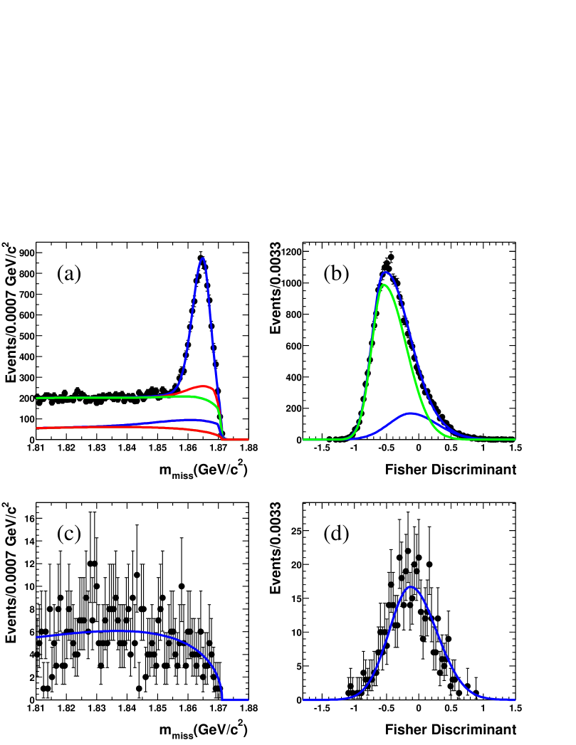
Figure 3: Result of the kinematic-variable fit for lepton-tagged events. The (a) $m_{\rm miss}$ and (b) Fisher discriminant $F$ distributions for the on-resonance data are shown by the points with error bars. In the $m_{\rm miss}$ plot, the overlayed curves show, from bottom to top, the cumulative contributions of continuum, peaking $B\kern 1.79993pt\overline{\kern-1.79993ptB}{}$, combinatoric $B\kern 1.79993pt\overline{\kern-1.79993ptB}{}$, $B^{0}\rightarrow D^{*+}\rho^{-}$ and $B^{0}\rightarrow D^{*+}\pi^{-}$ events. In the $F$ plot, the PDFs for $B\kern 1.79993pt\overline{\kern-1.79993ptB}{}$ and continuum events are overlaid. Plots (c) and (d) show the same distributions for off-resonance data.

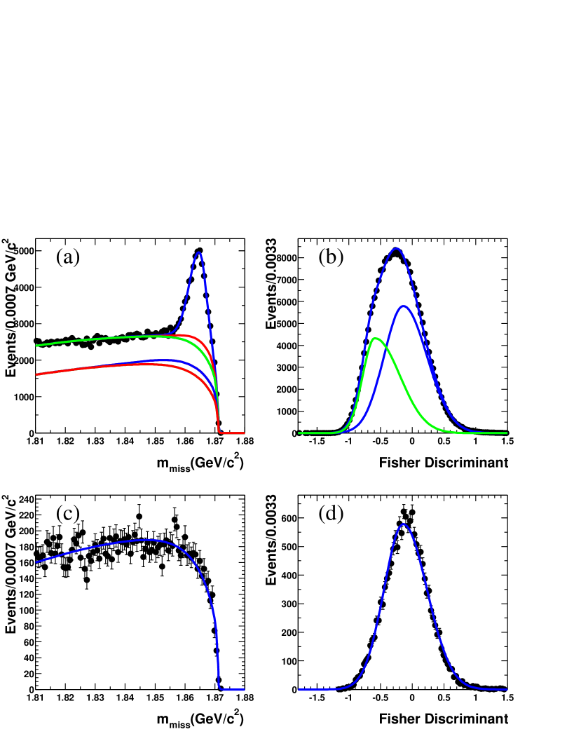
Figure 4: Result of the kinematic-variable fit for kaon-tagged events. The (a) $m_{\rm miss}$ and (b) Fisher discriminant $F$ distributions for the on-resonance data are shown by the points with error bars. In the $m_{\rm miss}$ plot, the overlayed curves show, from bottom to top, the cumulative contributions of continuum, peaking $B\kern 1.79993pt\overline{\kern-1.79993ptB}{}$, combinatoric $B\kern 1.79993pt\overline{\kern-1.79993ptB}{}$, $B^{0}\rightarrow D^{*+}\rho^{-}$ and $B^{0}\rightarrow D^{*+}\pi^{-}$ events. In the $F$ plot, the PDFs for $B\kern 1.79993pt\overline{\kern-1.79993ptB}{}$ and continuum events are overlaid. Plots (c) and (d) show the same distributions for off-resonance data.

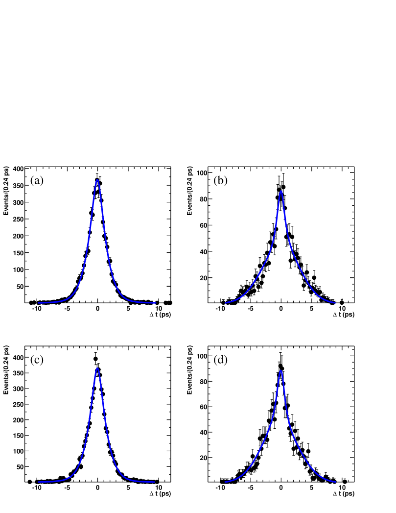
Figure 5: Result of the $\Delta t$ fit to the lepton-tagged data in the signal region. The points with error bars show the $\Delta t$ distributions for (a) $B^{0}$-tag unmixed, (b) $B^{0}$-tag mixed, (c) $\kern 1.79993pt\overline{\kern-1.79993ptB}{}^{0}$-tag unmixed, (d) and $\kern 1.79993pt\overline{\kern-1.79993ptB}{}^{0}$-tag mixed events. The curves show the PDF with the parameters obtained from the fit.

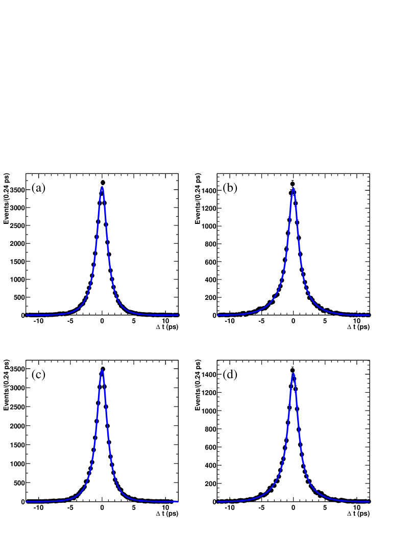
Figure 6: Result of the $\Delta t$ fit to the kaon-tagged data in the signal region. The points with error bars show the $\Delta t$ distributions for (a) $B^{0}$-tag unmixed, (b) $B^{0}$-tag mixed, (c) $\kern 1.79993pt\overline{\kern-1.79993ptB}{}^{0}$-tag unmixed, (d) and $\kern 1.79993pt\overline{\kern-1.79993ptB}{}^{0}$-tag mixed events. The curves show the PDF with the parameters obtained from the fit.

The fit to the signal region (Figs. 5 and 6), described in step 4 of Sec. 5, determines $\Delta m$, $\tau$, $\omega$, $\Delta\omega$, and the $C\!P$ parameters of the signal PDF $T_{D^{*}\pi}(\Delta t_{\rm true},s_{\rm tag},s_{\rm mix})$. These parameters are $S^{\pm}$ for lepton tags and $a$, $b$, $c$ for kaon tags. Five parameters of the signal resolution function are also determined by the fit, as are eight continuum parameters: four parameters for the $\Delta t_{\rm true}$ PDF and four parameters for the resolution function. The results of the fits on the data are

$$S^{+} = -0.078\pm 0.052~{}(stat.)\pm 0.020~{}(syst.),$$

$$S^{-} = -0.070\pm 0.052~{}(stat.)\pm 0.021~{}(syst.)$$ (30)

for the lepton-tagged events, and

$$a = -0.054\pm 0.032~{}(stat.)\pm 0.019~{}(syst.),$$

$$b = -0.009\pm 0.019~{}(stat.)\pm 0.011~{}(syst.),$$

$$c = +0.005\pm 0.031~{}(stat.)\pm 0.020~{}(syst.)$$ (31)

for the kaon-tagged events. We note the good agreement between $a$ and $(S^{+}+S^{-})/2$. The largest correlation of $S^{+}$ ($S^{-}$) with any linear combination of the other parameters floated in the fit is 0.24 (0.26) and the correlation between $S^{+}$ and $S^{-}$ is $-0.057$.

We define two time-dependent $C\!P$-violating asymmetries from the numbers of events observed at time $t$ with specific combinations of flavor tag and reconstructed final state:

$$\mathcal{A}^{rec}_{C\!P} = \frac{N({\rm tag~{}}B^{0},D^{*\pm}\pi^{\mp})(t)-N({\rm tag~{}}\kern 1.79993pt\overline{\kern-1.79993ptB}{}^{0},D^{*\pm}\pi^{\mp})(t)}{N({\rm tag~{}}B^{0},D^{*\pm}\pi^{\mp})(t)+N({\rm tag~{}}\kern 1.79993pt\overline{\kern-1.79993ptB}{}^{0},D^{*\pm}\pi^{\mp})(t)},$$

$$\mathcal{A}^{tag}_{C\!P} = \frac{N({\rm tag~{}}B^{0}+\kern 1.79993pt\overline{\kern-1.79993ptB}{}^{0},D^{*-}\pi^{+})(t)-N({\rm tag~{}}B^{0}+\kern 1.79993pt\overline{\kern-1.79993ptB}{}^{0},D^{*+}\pi^{-})(t)}{N({\rm tag~{}}B^{0}+\kern 1.79993pt\overline{\kern-1.79993ptB}{}^{0},D^{*-}\pi^{+})(t)+N({\rm tag~{}}B^{0}+\kern 1.79993pt\overline{\kern-1.79993ptB}{}^{0},D^{*+}\pi^{-})(t)}.$$ (32)

In the absence of background and experimental effects, $\mathcal{A}^{rec}_{C\!P}=-2r\sin(2\beta+\gamma)\cos\delta\sin(\Delta m\Delta t)$ and $\mathcal{A}^{tag}_{C\!P}=2r^{\prime}\sin(2\beta+\gamma)\cos\delta^{\prime}\sin(\Delta m\Delta t)$. The asymmetry plots obtained for the data in the signal region are shown in Fig. 8 for lepton tags and in Fig. 8 for kaon tags. As expected, no time-dependent asymmetry is visible for $\mathcal{A}^{tag}_{C\!P}$ in the lepton case.

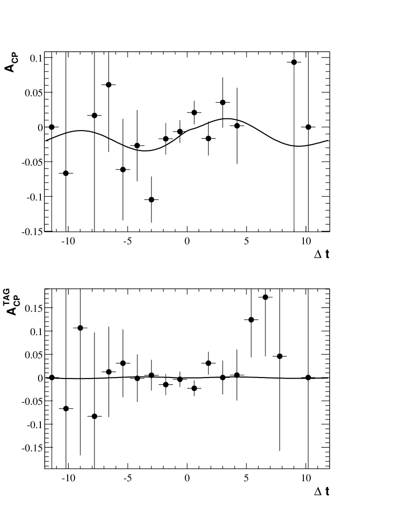
Figure 7: Raw asymmetries $\mathcal{A}^{rec}_{C\!P}$ and $\mathcal{A}_{C\!P}^{tag}$ (Eq. 32) for lepton tags as a function of $\Delta t$. The curves show the projection of the fitted PDF.

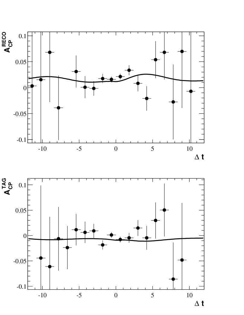
Figure 8: Raw asymmetries $\mathcal{A}^{rec}_{C\!P}$ and $\mathcal{A}_{C\!P}^{tag}$ (Eq. 32) for kaon tags as a function of $\Delta t$. The curves show the projection of the fitted PDF.

8 PHYSICS RESULTS

Combining $a$ and $(S^{+}+S^{-})/2$ from Eqs. 30 and  31, accounting for correlated errors, we obtain

$$2r\sin(2\beta+\gamma)\cos\delta=-0.063\pm 0.024~{}(stat.)\pm 0.017~{}(syst.).$$ (33)

This measurement deviates from 0 by 2.1 standard deviations, and is the main result of this analysis. From the difference $(S^{+}-S^{-})/2$, we obtain

$$2r\cos(2\beta+\gamma)\sin\delta=-0.004\pm 0.037~{}(stat.)\pm 0.020~{}(syst.).$$ (34)

We use two different methods for extracting constraints on $|\sin(2\beta+\gamma)|$ from our results. We emphasize that the two methods make use of different additional information and different assumptions, and are therefore not directly comparable. These constraints are interpretations of our experimental results. Each of the methods involves defining and minimizing a $\chi^{2}$ function of $\sin(2\beta+\gamma)$ and other parameters. The $\chi^{2}$ functions are symmetric under the exchange $\sin(2\beta+\gamma)\rightarrow-\sin(2\beta+\gamma)$. Due to the large uncertainties and the fact that the minimum value of the $\chi^{2}$ may occur at the boundary of the physical region ($|\sin(2\beta+\gamma)|=1$), the errors naively obtained from the variation of the $\chi^{2}$ functions are not relevant. In order to give a probabilistic interpretation to the results, we apply the Feldman-Cousins method [12] to set limits on $|\sin(2\beta+\gamma)|$.

In the first method we make no assumption regarding the value of $r$ and use no additional experimental information about $r$. In this method, for different values of $r$ we minimize the function

$$\chi^{2}=\sum_{j,k=1}^{3}\Delta x_{j}V^{-1}_{jk}\Delta x_{k},$$ (35)

where $\Delta x_{j}$ is the difference between the result of our measurement and the theoretical expression for $S^{+}$ ($j=1$), $S^{-}$ ($j=2$), and $a$ ($j=3$), and $V$ is the measurement error matrix, which is almost diagonal. The parameters determined by this fit are $\sin(2\beta+\gamma)$, which is limited to lie in the range $[-1,1]$, and $\delta$. The measurements of $b$ and $c$ are not used in the fit, since they depend on the unknown values of $r^{\prime}$ and $\delta^{\prime}$. We generate many parameterized MC experiments with the same sensitivity as reported here for different values of $\sin(2\beta+\gamma)$ and $r$. The fraction of these experiments in which $\chi^{2}(\sin(2\beta+\gamma))-\chi^{2}_{min}$ is smaller than in the data is computed and interpreted as the confidence level (CL) of the lower limit on $|\sin(2\beta+\gamma)|$. The 90% and 95% CL limits as a function of $r$ are shown in Fig. 9. The $\chi^{2}$ fit determines $|\sin(2\beta+\gamma)|$ up to the twofold ambiguity $|\sin(2\beta+\gamma)|\leftrightarrow|\cos\delta|$. The limits shown in Fig. 9 are always the more conservative of the two possibilities.

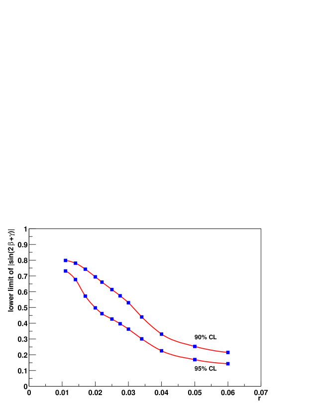
Figure 9: The 90% and 95% CL lower limits on $|\sin(2\beta+\gamma)|$ as a function of $r$, using no experimental information on $r$.

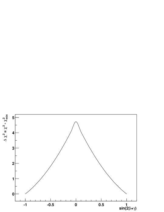
Figure 10: $\tilde{\chi}^{2}-\tilde{\chi}^{2}_{min}$ as a function of $\sin(2\beta+\gamma)$, assuming $r=0.017^{+0.005}_{-0.007}$ with an additional 30% non-Gaussian theoretical uncertainty.

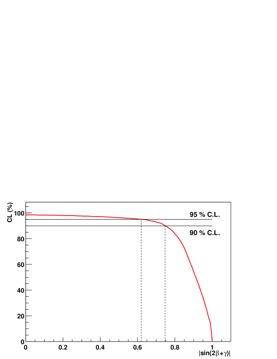
Figure 11: Confidence level (CL) as a function of the lower limit on $|\sin(2\beta+\gamma)|$, computed as the fraction of parameterized MC experiments where $\tilde{\chi}^{2}(\sin(2\beta+\gamma))-\tilde{\chi}^{2}_{min}$ is larger than in the data, with the assumptions of Fig. 10. The vertical lines correspond to 90% and 95% confidence level and lead to the bound $|\sin(2\beta+\gamma)|>0.75~{}(0.62)$ at the 90% (95%) CL.

In the second method we assume that $r$ may be estimated from

$$r=\tan\theta_{C}\,\sqrt{{\cal B}(B^{0}\rightarrow{D^{*}}_{s}^{+}\pi^{-})\over{\cal B}(B^{0}\rightarrow{D^{*}}^{-}\pi^{+})}\,{f_{D^{*}}\over f_{D^{*}_{s}}}$$ (36)

where $\theta_{C}$ is the Cabibbo angle. Using the branching fractions ${\cal B}(B^{0}\rightarrow{D^{*}}^{-}\pi^{+})=(0.276\pm 0.021)\%$ [7], ${\cal B}(B^{0}\rightarrow{D^{*}}_{s}^{+}\pi^{-})=(1.9{+1.2\atop-1.3}\pm 0.5)\times 10^{-5}$ [13] and the ratio of decay constants ${f_{D^{*}_{s}}\over f_{D^{*}}}=1.10\pm 0.02$ [14] yields

$$r=0.017^{+0.005}_{-0.007}.$$ (37)

An additional non-Gaussian 30% relative error is associated with the theoretical assumptions involved in obtaining this value. To carry out this method, we minimize

$$\tilde{\chi}^{2}=\sum_{j,k=1}^{3}\Delta x_{j}V^{-1}_{jk}\Delta x_{k}+\Delta^{2}(r),$$ (38)

where the function

$$\Delta^{2}(r)=\left\{\matrix{\left({r-r_{0}\over 0.005}\right)^{2}&&(r-r_{0})/r_{0}>0.3,\cr 0&&|r-r_{0}|/r_{0}\leq 0.3,\cr\left({r-r_{0}\over 0.007}\right)^{2}&&(r-r_{0})/r_{0}<-0.3}\right.$$ (39)

accounts for the 30% theoretical error and the Gaussian experimental error around the central value $r=r_{0}$, Eq. 38. In addition to $\sin(2\beta+\gamma)$ and $\delta$, the parameter $r$ is also determined by this fit. The minimum of $\tilde{\chi}^{2}$ occurs at $|\sin(2\beta+\gamma)|=1.0$, $\delta=0$, and $r=0.024$, and at a value of $\tilde{\chi}^{2}_{min}=0.54$ for one degree of freedom. The value of $\tilde{\chi}^{2}-\tilde{\chi}^{2}_{min}$ as a function of $\sin(2\beta+\gamma)$ and the resulting Feldman-Cousins confidence level curve are shown in Figs. 10 and 11. This method yields the limits $|\sin(2\beta+\gamma)|>$0.88 at 68% CL, $|\sin(2\beta+\gamma)|>$0.75 at 90% CL, and $|\sin(2\beta+\gamma)|>$0.62 at 95% CL.

9 SUMMARY

We present preliminary results of a study of time-dependent $C\!P$ asymmetries in the $B^{0}\rightarrow D^{*\mp}\pi^{\pm}$ decay channels using the partial reconstruction method. The time-dependent $C\!P$ asymmetry that we measure,

$$2r\sin(2\beta+\gamma)\cos\delta=-0.063\pm 0.024~{}(stat.)\pm 0.017~{}(syst.),$$ (40)

is different from 0 by 2.1 standard deviations. This asymmetry does not depend on assumptions regarding $r$, the ratio of the magnitudes of the $b\rightarrow u\bar{c}d$ and $b\rightarrow c\bar{u}d$ amplitudes contributing to this decay. We present model-independent bounds on $|\sin(2\beta+\gamma)|$ as a function of $r$. With some assumptions regarding $r$, our results can be interpreted as a limit on the combination of CKM angles $2\beta+\gamma$, $|\sin(2\beta+\gamma)|>0.75~{}(0.62)$ at the 90% (95%) CL.

10 ACKNOWLEDGMENTS

We are grateful for the extraordinary contributions of our PEP-II colleagues in achieving the excellent luminosity and machine conditions that have made this work possible. The success of this project also relies critically on the expertise and dedication of the computing organizations that support BABAR. The collaborating institutions wish to thank SLAC for its support and the kind hospitality extended to them. This work is supported by the US Department of Energy and National Science Foundation, the Natural Sciences and Engineering Research Council (Canada), Institute of High Energy Physics (China), the Commissariat à l’Energie Atomique and Institut National de Physique Nucléaire et de Physique des Particules (France), the Bundesministerium für Bildung und Forschung and Deutsche Forschungsgemeinschaft (Germany), the Istituto Nazionale di Fisica Nucleare (Italy), the Foundation for Fundamental Research on Matter (The Netherlands), the Research Council of Norway, the Ministry of Science and Technology of the Russian Federation, and the Particle Physics and Astronomy Research Council (United Kingdom). Individuals have received support from the A. P. Sloan Foundation, the Research Corporation, and the Alexander von Humboldt Foundation.

References

- [1] N. Cabibbo, Phys. Rev. Lett. 10, 531 (1963); M. Kobayashi and T. Maskawa, Prog. Theoret. Phys. 49, 652 (1973).
- [2] R.G. Sachs, Enrico Fermi Institute Report, EFI-85-22 (1985) (unpublished); I. Dunietz and R.G. Sachs, Phys. Rev. D37 (1988), 3186 [E: Phys. Rev. D39, 3515 (1989)]; I. Dunietz, Phys. Lett. B427, 179 (1998); P.F. Harrison and H.R. Quinn, ed., “The BABAR Physics Book”, SLAC-R-504 (1998), Chap. 7.6.
- [3] The CLEO Collaboration, G. Brandenburg et al., Phys. Rev. Lett. 80, 2762 (1998).
- [4] The BABAR Collaboration, B. Aubert et al., Phys. Rev. D 67, 091101 (2003).
- [5] Robert Fleischer (2003), arXiv:hep-ph/0304027.
- [6] The BABAR Collaboration, B. Aubert et al., Nucl. Instrum. Methods A479, 1 (2002).
- [7] Particle Data Group, K. Hagiwara et al. Phys. Rev. D 66, 010001 (2002).
- [8] G. Fox and S. Wolfram, Phys. Rev. Lett. 41, 1581 (1978).
- [9] R. A. Fisher, Annals of Eugenics 7, 179 (1936); M.S. Srivastava and E.M. Carter, “An Introduction to Applied Multivariate Statistics”, North Holland, Amsterdam (1983).
- [10] O. Long, M. Baak, R.N. Cahn, and D. Kirkby, SLAC-PUB-9687, arXiv:hep-ex/0303030, to appear in Phys. Rev. D.
- [11] The BABAR Collaboration, B. Aubert et al., Phys. Rev. D 66, 032003 (2002).
- [12] G. Feldman and R. Cousins, Phys. Rev. D 57, 3873 (1998).
- [13] The BABAR Collaboration, B. Aubert et al., arXiv:hep-ex/0207053.
- [14] D. Becirevic, Nucl. Phys. Proc. Suppl. 94, 337 (2001).