Evidence for Two-Body Hadronic Decays of the $\Upsilon$ 

Abstract

We describe a search for hadronic decays of the $\Upsilon$(1S), $\Upsilon$(2S), and $\Upsilon$(3S) resonances to the exclusive final states $\rho\pi$, $K^{*}(892)\bar{K}$, $\rho a_{2}(1320)$, $\omega f_{2}(1270)$, $\phi f_{2}^{\prime}(1525)$, $K^{*}(892)\bar{K}^{*}_{2}(1430)$, $b_{1}(1235)\pi$, $K_{1}(1270)\bar{K}$, and $K_{1}(1400)\bar{K}$. Upper limits at 90% CL are set for all these decays from all three resonances below $33\times 10^{-6}$; in particular, $\cal{B}$($\Upsilon$(1S)$\to\rho\pi)~{}<~{}4\times 10^{-6}$ is the smallest such upper limit. For two modes, a branching fraction of zero can be ruled out with a statistical significance of more than $5\sigma$: $B(\Upsilon(1S)\to\phi f_{2}^{\prime}(1525))=(7^{+3}_{-2}\pm 1)\times 10^{-6}$ and $B(\Upsilon(1S)\to K_{1}(1400)\bar{K})=(14^{+4}_{-3}\pm 2)\times 10^{-6}$. Production of $K_{1}(1270)\bar{K}$ in $\Upsilon$(1S) decay is suppressed relative to that of $K_{1}(1400)\bar{K}$. These results add another piece to the challenging “$\rho-\pi$ puzzle” of the charmonium system, placing constraints on models of how quantum chromodynamics should be applied to heavy quarkonia. All results are preliminary.

I Introduction and Motivation

Little experimental information exists on exclusive decays of the $\Upsilon$ resonances below $B\bar{B}$ threshold. Upper limits have been published for the decays $\Upsilon(1S)\to\rho\pi$ and $\Upsilon(1S)\to h\bar{h}$, $h=\pi,\ K,\ p$, all of the order $10^{-4}$, and $\Upsilon(1S)\to\pi^{+}\pi^{-}\pi^{0}$ ($1.8\times 10^{-5}$) pdg2002 . No exclusive final states for the $\Upsilon(2S)$ and $\Upsilon(3S)$ have been examined. The situation is different in charmonium, where numerous channels have been measured. This by itself poses a motivation to study hadronic $\Upsilon$ decays, given the similarity of these two strongly-bound heavy quark systems. Furthermore, a long-standing unsolved puzzle in charmonium regarding the ratio of branching fractions of the $2^{3}S_{1}$ ($\psi^{\prime}$) and $1^{3}S_{1}$ ($J/\psi$) to final states consisting of a pseudoscalar and a vector warrants the corresponding measurement in bottomonium.

The expectation that the dilepton and hadronic ratios of decay widths should be at least roughly equal follows from QED and QCD. Both processes are thought to occur via annihilation of the constituent quark and antiquark, in one case to a photon and in the other to three gluons, and therefore are both proportional to the square of the quark-antiquark wave function overlap at the origin. Restating the QCD expectation for hadronic decays in terms of ratios of branching fractions instead of decay widths, and neglecting the running of the strong coupling constant, one obtains the following prediction regarding an arbitrary final state $H$:

$$Q=\frac{{\cal B}(\psi(2S)\to H)}{{\cal B}(J/\psi\to H)}\approx\frac{{\cal B}(\psi(2S)\to e^{+}e^{-})}{{\cal B}(J/\psi\to e^{+}e^{-})}$$ (1)

Using the leptonic branching fractions ${\cal B}(J/\psi\to e^{+}e^{-})=(5.93\pm 0.1)\times 10^{-2}$ and ${\cal B}(\psi(2S)\to e^{+}e^{-})=(7.3\pm 0.4)\times 10^{-3}$ pdg2002 , the expected value for the ratio is $(12.3\pm 0.9)\%$.

A number of channels have been studied, most of which satisfy the prediction within experimental errors. The most significant deviation known so far comes from the following vector-pseudoscalar ($VP$) and vector-tensor ($VT$) final states pdg2002 : $\rho\pi$ ($Q<0.007$), $K^{*}(892)\bar{K}$ ($Q<0.001$), $\rho a_{2}(1320)$ ($Q<0.02$), $K^{*}(892)\bar{K_{2}^{*}}(1430)$ ($Q<0.02$), and $\omega f_{2}(1270)$ ($Q<0.03$ BESPsiprimedecays ; pdg2002 ).

Many theoretical approaches have been made to resolve this puzzle. None is able to accommodate all the measurements reported so far. For some, the crucial question is whether the $J/\psi$ is enhanced or the $\psi^{\prime}$ is suppressed. Therefore, in addition to adding experimental information to the scarce amount that is available at this point on $J^{PC}=1^{--}$ bottomonium decays, in particular in the $\rho\pi$ channel, it is an interesting question what the ratio analog to Equation 1 should turn out to be for the $\Upsilon$ system.

Depending on which theoretical model is used to explain the behavior measured in charmonium, the expectation for bottomonium varies. A common assumption is that the individual branching fractions in bottomonium should be at least one order of magnitude smaller than in charmonium. How much they are smaller should be of some utility in deciphering the puzzle.

Two important features distinguish the situation in bottomonium from that in charmonium. First, in addition to the comparison of the 2S excitation with the ground state, the 3S resonance can be used due to the fact that it is below open flavor production threshold, in contrast to the situation in charmonium. Furthermore, the ratio predicted based on Equation 1 is $48\%$ for $\mbox{$\Upsilon(2S)$}:\mbox{$\Upsilon(1S)$}$ and $72\%$ for $\mbox{$\Upsilon(3S)$}:\mbox{$\Upsilon(1S)$}$.

CLEO recently accumulated several million bottomonium decays at each of the $\Upsilon(1S)$, $\Upsilon(2S)$, and $\Upsilon(3S)$ resonances. These datasets can probe decays of the $J^{PC}=1^{--}$ $b\bar{b}$ bound states at the $10^{-5}$ level. The decays pursued in this work are $\rho\pi$, $K^{*}(892)\bar{K}$, $\rho a_{2}(1320)$, $\omega f_{2}(1270)$, $\phi f_{2}^{\prime}(1525)$, $K^{*}(892)K_{2}^{*}(1430)$, $b_{1}(1235)\pi$, $K_{1}(1270)\bar{K}$, and $K_{1}(1400)\bar{K}$. They sample $VP$, axialvector-pseudoscalar ($AP$), and $VT$ type final states with and without strangeness and constitute the most copious two-body hadronic final states in $J/\psi$ decay (each with a branching ratio of $0.1-1\%$). Each proceeds via the strong interaction and conserves isospin. These decay modes provide a logical starting point for using the $\Upsilon$ system to untangle the many subleties of the $\rho\pi$ puzzle and associated anomalies.

II Analysis overview

The analysis strategy is straightforward. Event selection criteria for the different modes are developed using signal Monte Carlo. We emphasize cleanliness over efficiency in order to suppress decays faking the desired final states. CLEO data taken at and just below the $\Upsilon(4S)$ resonance, suitably scaled by luminosity and beam energy, is used as an indication of background properties and final contamination levels. Finally, projected backgrounds and event totals are normalized by efficiencies and the number of resonance decays produced, and branching fractions or upper limits computed.

It is important to note that many different kinds of backgrounds contribute to the sample obtained at the $\Upsilon(4S)$ resonance. Not all of them scale with the same center-of-mass energy dependence (see discussion below). For that portion of backgrounds which are truly the same final state but produced non-resonantly, that is, proceed as $e^{+}e^{-}\to\gamma^{*}\to H$ instead of $e^{+}e^{-}\to\Upsilon\to H$, there is also the possibility of interference, which has been neglected in this work.

III Event Selection

The CLEO III detector is described in detail in cleoiiidetector . Its key features exploited in this analysis are a solid angle coverage for charged and neutral particles of 93% and two particle identification systems to separate kaons from pions, namely using energy loss in the drift chamber and a Ring Imaging Cherenkov detector RICHNIM . The tracking system achieves a charged particle momentum resolution of 0.35% (1%) at $p=$1 GeV/$c$ ($p=$5 GeV/$c$) and the calorimeter a photon energy resolution of 2.2% (1.5%) at $E_{\gamma}=$1 GeV ($E_{\gamma}=$5 GeV). The combined $dE/dx$-RICH particle identification system attains a kaon efficiency (fake rate) $>$90% ($<5$%) below 2.5 GeV/$c$ and falls (rises) to $\sim$70% ($\sim$25%) near 5 GeV/$c$.

Standard requirements are used to identify charged particles from tracks in the drift chamber and photons from electromagnetic showers in the CsI calorimeter. The simplicity of the final states under study is exploited by imposing an energy conservation requirement on $X_{T}=\Sigma_{h}(E_{h})/(2E_{beam})$ of $0.98\leq X_{T}\leq 1.015$ when summing over the energies of the decay products. For all the target modes, the experimental resolution in this quantity is smaller than $1\%$. For each of the final state resonances, a search window for the invariant mass of the decay products is established based on signal Monte Carlo studies. Electron and muon vetoes are imposed to suppress QED backgrounds.

IV Monte Carlo samples

Efficiencies are evaluated with Monte Carlo simulation of the process and detector response GEANT . The $\rho\pi$ and $K^{*}\bar{K}$ modes are generated with the polar angle $\theta$ distributed according to $(1+\cos^{2}\theta)$. All other channels are thrown to be flat in $\cos\theta$ as they can be of any linear combination of $\sin^{2}\theta$ and ($1+\cos^{2}\theta$). The final efficiencies are of the order of $5-10\%$, including all effects of selection criteria and all intermediate branching fractions (Table 1). The detection efficiency of some of the modes varies significantly with the beam energy and so is evaluated at the $\Upsilon(1S)$ and $\Upsilon(4S)$ separately. The $\Upsilon(2S)$ and $\Upsilon(3S)$ efficiencies, also listed in Table 1, are obtained by interpolating linearly between the $\Upsilon(1S)$ and $\Upsilon(4S)$.

Systematic uncertainties on the efficiency include uncertainties in the polar angle distribution for $VT$ and $AP$ modes (5%) and modeling of tracks (1% per charged track), $\pi^{0}$s (8% per beam-energy-$\pi^{0}$ and 5% per softer $\pi^{0}$), lepton veto (1% per particle), kaon identification (5% per identified kaon) and pion fake rate (3%), and secondary vertex-finding (5%). These contributions and the uncertainty in the number of produced $\Upsilon$ decays ($5\%$) are summed in quadrature. The resulting total relative error is close to $10\%$ for all modes.

Although $\tau$-pair production of the states in question contributes for $X_{T}<0.98$, the background in the signal region is found to be small, as is that from $\mu$-pairs.

V Determination of signal and background yield

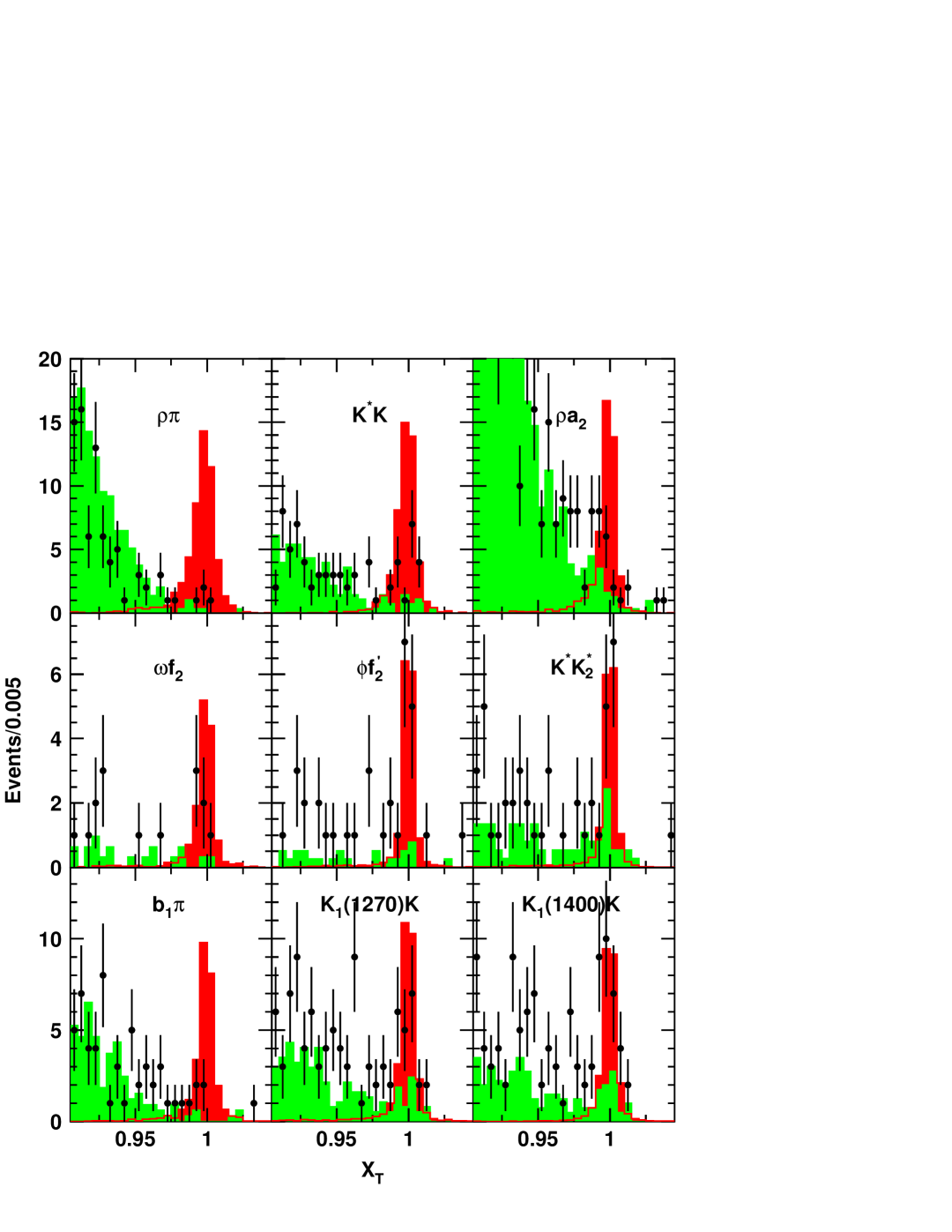
Figure 1: Scaled total energy, $X_{T}$, distribution for candidate channels from $\Upsilon$(1S), in which all selection criteria $except$ the $X_{T}$ requirement have been applied. Solid points represent data; the red (dark) histogram is signal MC with arbitrary normalization; the green (light) histogram is scaled 4S data.

The data samples used consist of ($21\pm 1$), ($5.4\pm 0.2$), and ($5.0\pm 0.3$) $\times 10^{6}$ $\Upsilon(1S)$, $\Upsilon(2S)$, and $\Upsilon(3S)$ decays, respectively. Events that satisfy the event selection criteria mentioned in the previous section are simply counted. To obtain maximal statistical power, both charged and neutral decay modes were considered and combined for the final result. The uncorrected event numbers thus obtained are listed in Table 2. Example distributions of the scaled total energy and invariant masses for the nine channels under study for $\Upsilon(1S)$ decays can be found in Figures 1 and 2.

The background level was determined using a large amount of data taken on or near the $\Upsilon(4S)$ resonance, extrapolated down to the lower resonances. For the extrapolation, three issues must be taken into account: Scaling with luminosity, efficiency dependence on the center-of-mass energy, and cross section dependence on the center-of-mass energy. The efficiency dependence can be read off Table 1. The ratio of integrated luminosities for the datasets used is 0.133, 0.093, and 0.135 for $\mbox{$\Upsilon(1S)$}:\mbox{$\Upsilon(4S)$}$, $\mbox{$\Upsilon(2S)$}:\mbox{$\Upsilon(4S)$}$, and $\mbox{$\Upsilon(3S)$}:\mbox{$\Upsilon(4S)$}$, respectively. The cross section extrapolation with beam energy poses the most uncertain contribution. Depending on the contributing background process, it could vary from $1/s$ for QED processes to as much as $1/s^{3}$ ($1/s^{4}$ for $VP$ channels such as $\rho\pi$ or $K^{*}\bar{K}$).BRODLEP We therefore quote ranges of scale factors that take this uncertainty into account, shown in Table 3. The scale factors vary between $0.10$ and $0.45$. Within a specific channel, the ratio of upper to lower scale factor limit ranges from a maximum of almost $2$ for the $\Upsilon(1S)$ $VP$ modes down to the level of $1.1$ for $\Upsilon(3S)$ channels.

Cross-feed between the investigated final states is accounted for as a separate source of background. The largest contribution is found to be $K_{1}(1400)\bar{K}$ events leaking into the $K_{1}(1270)\bar{K}$ sample. The $K_{1}(1400)\bar{K}$ signal above $M(K\pi\pi)=1.4~{}GeV$ (where there is no $K_{1}(1270)$ signal) is evaluated with only the $\Upsilon(4S)$ background considered and then, scaled in accordance to the Monte Carlo detection efficiency, taken as a second source of background for the $K_{1}(1270)\bar{K}$. We neglect cross-feed in the other direction because the predicted backgrounds to $K_{1}(1270)\bar{K}$ saturate the observed rate. Also, the $\rho\pi$ channel receives contributions from mis-identified $K^{*}(892)\bar{K}$ events in the $\rho^{-}\pi^{+}$ mode. Again, the $K^{*}(892)\bar{K}$ leakage is treated as a second source of background, properly scaled. Using the $\Upsilon(4S)$ event yield from Table 2 together with the maximal scale factors from Table 3, and, where necessary, scaled cross-feed contributions, one arrives at estimates of background levels listed in Table 4.

The confidence level that any given mean signal combined with background would exceed or equal the observed event count is computed from simulated trials in which a pseudo-random number generator is employed to throw Poisson distributions. Poisson fluctuations in both the observed resonance and 4S samples are simulated by allowing not only the background to vary around its mean from one trial to the next, but also the mean background itself: 4S levels are fluctuated around the observed number prior to application of the scale factor to obtain the mean, and only then are fluctuations on the mean introduced. We reject thrown backgrounds which exceed the number of observed events. Trials are thrown in steps of 0.1 in signal mean until the desired confidence level is exceeded. This procedure predicts slightly larger intervals than the approach by Feldman and Cousins FELDCOUS when backgrounds are less than the observed number of events, and considerably wider ones for observations smaller than the mean expected background.

Upper limits at $90\%$ CL on the number of signal events are listed in Table 5, for which the $1/s$ scale factors were used to minimize the estimated non-resonant background and therefore to maximize any potential signal. These are converted into $90\%$ CL upper limits on the corresponding branching fractions shown in Table 6 using the number of produced resonance decays and efficiencies (Table 1); we account for the systematic relative error of $10\%$ in this conversion by increasing each upper limit by an additional $1.28\sigma\cong 13\%$.

Two-sided intervals of $68\%$ confidence level are also shown in Table 6 for channels with statistical significance exceeding one standard deviation. We define the statistical significance to be the number of Gaussian standard deviations above which lies the probability that the background alone fluctuated up to the observed number of events. For these intervals, the upper end of the 4S scale factor range is employed to minimize the chance of undersubtracting background. The systematic error shown includes the uncertainty on the product of efficiency and number of $\Upsilon$’s produced mentioned above (10%) in quadrature with an additional 10% to account for uncertainties in $e^{+}e^{-}$ annihilation backgrounds as well as $\Upsilon$ cross-feed estimates. For two channels, $B(\mbox{$\Upsilon(1S)$}\to\phi f_{2}^{\prime}(1525))$ and $B(\mbox{$\Upsilon(1S)$}\to K_{1}(1400)\bar{K})$, zero branching fraction can be ruled out at a statistical significance of more than $5\sigma$, making these the first exclusive hadronic decay modes measured in the $\Upsilon$ system. Several other channels with significance near $\sim 3\sigma$ show suggestive but statistically marginal evidence for branching fractions at the few per million level.

In contrast to the $\psi(2S)$ and in similarity to the $J/\psi$ BESpsi' , the production of $K_{1}(1270)\bar{K}$ is suppressed relative to that of $K_{1}(1400)\bar{K}$.

VI Conclusions

Using CLEO III datasets of 21, 5.4, and 5.0 million $\Upsilon$(1S), $\Upsilon$(2S), and $\Upsilon$(3S) decays, respectively, we have searched for nine of the potentially most probable two-body-hadronic decays, which include $VP$, $AP$, and $VT$ channels: $\rho\pi$, $K^{*}(892)\bar{K}$, $\rho a_{2}(1320)$, $\omega f_{2}(1270)$, $\phi f_{2}^{\prime}(1525)$, $K^{*}(892)K_{2}^{*}(1430)$, $b_{1}(1235)\pi$, $K_{1}(1270)\bar{K}$, and $K_{1}(1400)\bar{K}$. The upper limit at 90% confidence level for $\Upsilon$(1S)$\to\rho\pi$ is lowered by more than an order of magnitude to $4\times 10^{-6}$, and 90% CL upper limits for the other eight modes, measured for the first time, range from $7-33\times 10^{-6}$. Two channels have been observed at convincing statistical significance: $B(\Upsilon(1S)\to\phi f_{2}^{\prime}(1525))=(7^{+3}_{-2}\pm 1)\times 10^{-6}$ and $B(\Upsilon(1S)\to K_{1}(1400)\bar{K})=(14^{+4}_{-3}\pm 2)\times 10^{-6}$. The branching fractions from the $\Upsilon$(1S) are smaller than the comparable values on the $J/\psi$ by factors of several hundred (for $K_{1}(1400)\bar{K}$) to at least several thousand (for $\rho\pi$); the $\Upsilon(1S)\to\rho\pi$ branching fraction is measured to be suppressed by at least six powers of $M_{J/\psi}/M_{\Upsilon}$ relative to $J/\psi\to\rho\pi$. The above results are preliminary.

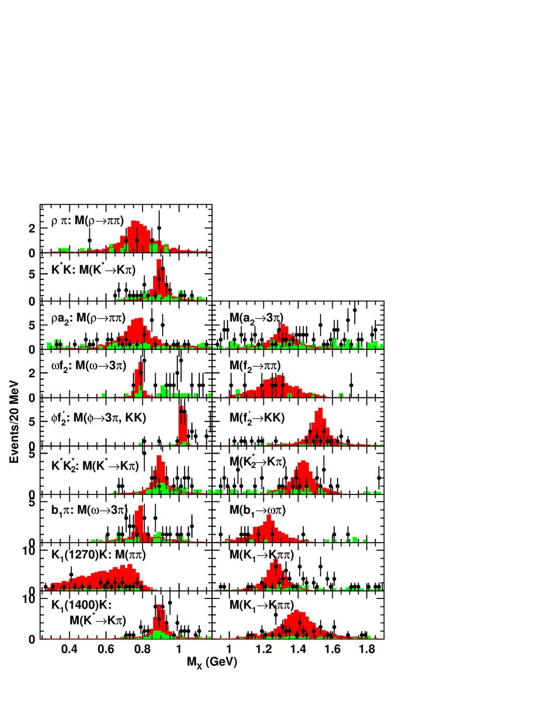
Figure 2: Mass distributions of intermediate states $M_{X}$, with $X$ given by the label in parentheses, for candidate channels from $\Upsilon$(1S) decays, in which all selection criteria $except$ the one on the plotted mass have been applied. Solid points represent data; the red (dark) histogram is signal MC with arbitrary normalization; the green (light) histogram is scaled 4S data. Plots on the right refer to the same channel as each neighboring plot on the left.

Table 1: Efficiency in percent for the isospin- and charge-conjugate-inclusive parent decay channels listed, summed over the various sub-modes used in this analysis, including all the effects of selection criteria and all intermediate branching fractions.

Channel	$\Upsilon$(1S)	$\Upsilon$(2S)	$\Upsilon$(3S)	4S
$\rho~{}\pi$	7.8	6.6	6.0	5.6
$K^{*}(892)~{}\bar{K}$	10.6	10.0	9.6	9.5
$\rho~{}a_{2}(1320)$	7.8	7.0	6.6	6.3
$\omega~{}f_{2}(1270)$	7.7	6.9	6.5	6.1
$\phi~{}f_{2}^{\prime}(1535)$	10.1	10.1	10.2	10.2
$K^{*}(892)~{}\bar{K}_{2}^{*}(1430)$	5.3	5.2	5.1	5.1
$b_{1}(1235)~{}\pi$	7.2	6.6	6.2	6.0
$K_{1}(1270)~{}\bar{K}$	9.2	8.9	8.7	8.6
$K_{1}(1400)~{}\bar{K}$	9.4	9.3	9.3	9.3

Table 2: Number of events in each isospin- and charge-conjugate-inclusive decay channel.

Channel	$\Upsilon$(1S)	$\Upsilon$(2S)	$\Upsilon$(3S)	4S
$\rho~{}\pi$	4	1	3	6
$K^{*}(892)~{}\bar{K}$	18	2	4	15
$\rho~{}a_{2}(1320)$	29	8	10	47
$\omega~{}f_{2}(1270)$	6	1	0	4
$\phi~{}f_{2}^{\prime}(1535)$	17	4	0	7
$K^{*}(892)~{}\bar{K}_{2}^{*}(1430)$	16	6	5	23
$b_{1}(1235)~{}\pi$	6	1	2	3
$K_{1}(1270)~{}\bar{K}$	27	7	8	29
$K_{1}(1400)~{}\bar{K}$	37	13	9	38

Table 3: Range of scale factors for the 4S yield to the lower resonances for the combined isospin-and charge-conjugate-inclusive decay channels, including luminosity, efficiency energy dependence, and range of $1/s^{n}$ scaling (see text).

Channel	$\Upsilon$(1S)	$\Upsilon$(2S)	$\Upsilon$(3S)
$\rho~{}\pi$	0.23-0.45	0.12-0.17	0.15-0.17
$K^{*}(892)~{}\bar{K}$	0.19-0.36	0.13-0.15	0.14-0.16
$\rho~{}a_{2}(1320)$	0.21-0.32	0.11-0.14	0.15-0.16
$\omega~{}f_{2}(1270)$	0.21-0.32	0.12-0.14	0.15-0.16
$\phi~{}f_{2}^{\prime}(1535)$	0.17-0.26	0.12-0.13	0.14-0.15
$K^{*}(892)~{}\bar{K}_{2}^{*}(1430)$	0.17-0.27	0.12-0.13	0.14-0.15
$b_{1}(1235)~{}\pi$	0.20-0.31	0.11-0.14	0.15-0.16
$K_{1}(1270)~{}\bar{K}$	0.17-0.27	0.12-0.13	0.14-0.15
$K_{1}(1400)~{}\bar{K}$	0.16-0.25	0.12-0.13	0.14-0.15

Table 4: Approximate background level estimate(s) from non-resonant $e^{+}e^{+}-$ annihilation scaled from the 4S data, and, where indicated by a “+”, cross-feed from other channels (see text), in the isospin- and charge-conjugate-inclusive decay channels.

Channel	$\Upsilon$(1S)	$\Upsilon$(2S)	$\Upsilon$(3S)
$\rho~{}\pi$	3+2	1+0	1+0
$K^{*}(892)~{}\bar{K}$	5	2	2
$\rho~{}a_{2}(1320)$	15	7	8
$\omega~{}f_{2}(1270)$	1	0.6	0.6
$\phi~{}f_{2}^{\prime}(1525)$	2	1	1
$K^{*}(892)~{}\bar{K}_{2}^{*}(1430)$	6	3	4
$b_{1}(1235)~{}\pi$	1	0.4	0.5
$K_{1}(1270)~{}\bar{K}$	8+20	4+8	4+4
$K_{1}(1400)~{}\bar{K}$	10	5	6

Table 5: Upper limits on number of signal events seen in each channel, at 90% confidence level, computed using the observed 4S yield with the lower end of the range of scale factors (i.e. based on a $1/s$ cross-section dependence, resulting in a low background prediction), and including the statistical fluctuations of not only signal and background but also the mean of the background.

Channel	$\Upsilon$(1S)	$\Upsilon$(2S)	$\Upsilon$(3S)
$\rho~{}\pi$	5.5	3.5	5.9
$K^{*}(892)~{}\bar{K}$	22.1	4.0	6.1
$\rho~{}a_{2}(1320)$	27.6	8.1	8.8
$\omega~{}f_{2}(1270)$	9.8	3.6	2.3
$\phi~{}f_{2}^{\prime}(1535)$	22.5	7.3	2.3
$K^{*}(892)~{}\bar{K}_{2}^{*}(1430)$	18.7	8.0	6.4
$b_{1}(1235)~{}\pi$	10.0	3.7	5.0
$K_{1}(1270)~{}\bar{K}$	13.3	4.6	6.7
$K_{1}(1400)~{}\bar{K}$	40	14.5	9.2

Table 6: $\Upsilon$ branching fraction 68% confidence intervals and 90% CL upper limits, in units of 10^-6, for each isospin- and charge-conjugate-inclusive decay channel. The first error is statistical and the second is systematic. For the 90% CL upper limits, a low-end 4S scale factor was used, whereas for the 68% confidence intervals the maximal scale factor value was employed. Also shown is the statistical signal significance (in units of $\sigma$). A “$-$” indicates less than 1$\sigma$ significance, defined as the number of Gaussian standard deviations above which lies the probability that the background alone fluctuated up to the observed number of events.

Channel	$\Upsilon$(1S)		$\Upsilon$(2S)		$\Upsilon$(3S)
	Interval/Sig.	UL	Interval/Sig.	UL	Interval/Sig.	UL
$\rho~{}\pi$	$-$	4	$-$	11	9${}_{-8}^{+7}\pm 1$ / 1.5	22
$K^{*}(892)~{}\bar{K}$	6${}_{-2}^{+3}\pm 1$ / 3.6	11	$-$	8	$-$	14
$\rho~{}a_{2}(1320)$	9$\pm 4\pm 1$ / 3.0	19	$-$	24	8${}_{-~{}6}^{+15}\pm 1$ / 1.3	30
$\omega~{}f_{2}(1270)$	3${}_{-1}^{+2}\pm 1$ / 2.6	7	$-$	11	$-$	8
$\phi~{}f_{2}^{\prime}(1525)$	7${}_{-2}^{+3}\pm 1$ / 5.5	12	6${}_{-3}^{+6}\pm 1$ / 3.0	17	$-$	14
$K^{*}(892)~{}\bar{K}_{2}^{*}(1430)$	9${}_{-4}^{+5}\pm 1$ / 3.0	19	11$\pm 8\pm 2$ / 1.6	32	$-$	28
$b_{1}(1235)~{}\pi$	3$\pm 2\pm 1$ / 2.9	8	$-$	12	5${}_{-4}^{+9}\pm 1$ / 1.4	18
$K_{1}(1270)~{}\bar{K}$	$-$	8	$-$	11	$-$	17
$K_{1}(1400)~{}\bar{K}$	14${}_{-3}^{+4}\pm 2$ / 5.6	23	16${}_{-~{}7}^{+10}\pm 2$ / 2.9	33	7${}_{-~{}5}^{+10}\pm 1$ / 1.5	22