Heavy Flavour Lifetimes and Lifetime Differences

Abstract

We give an overview of heavy flavour lifetime measurements, focusing on recent results from the Tevatron and the B factories.

1 Introduction

In the first part of this article we summarise the status and latest measurements of B-hadron lifetimes and lifetime ratios, including some recent result from the Tevatron and the B factories, and compare those results with the predictions from Heavy Quark Expansion (HQE). Future prospects for lifetime measurements at the B factories and the Tevatron are discussed.

In the second part, we review the status and prospects of measuring the difference between the lifetimes of the two CP eigenstates in the ${\rm B_{s}^{0}}$-${\rm\overline{B_{s}^{0}}}$ system.

2 Lifetimes and Lifetime Ratios

2.1 Theoretical Predictions on B Hadron Lifetimes

Life time measurements in the heavy quark sector gain specific significance due to the precise predictions of Heavy Quark expansion (see e.g. [1], [2]) thus providing a testing ground for this theoretical tool that is frequently used, for example to relate experimental measurements to CKM parameters like $\Gamma_{d}$ to $\left|V_{cb}\right|$ or $\Delta m_{s}/\Delta m_{d}$ to $\left|V_{ts}/V_{td}\right|$.

The hierachy expected for b hadron lifetimes is [3]:

$$\tau({\rm B_{c}})\ll\tau(\Xi_{b}^{0})$$

$$\color[rgb]{1,0,0}\sim\tau({\rm\Lambda_{b}})<\tau({\rm B_{d}^{0}})\sim\tau({\rm B_{s}^{0}})<\tau({\rm B^{-}})$$

$$<\tau({\rm\Xi_{b}^{-}})<\tau({\rm\Omega_{b}}).$$

Recent HQE predictions for the lifetime ratios are [4]:

• $\tau({\rm B^{-}})/\tau({\rm B_{d}^{0}})=1.06\pm 0.02$

• $\tau({\rm B_{s}})/\tau({\rm B_{d}^{0}})=1.00\pm 0.01$

• $\tau({\rm\Lambda_{b}})/\tau({\rm B_{d}^{0}})=0.90\pm 0.05$

2.2 The B Factories

The B factories BaBar and Belle at the asymmetric ${\rm e^{+}e^{-}}$ colliders PEP-II and KEK have collected $\mathrm{123\,fb^{-1}}$ and $\mathrm{145\,fb^{-1}}$ worth of data respectively up to May 2003, running at the ${\rm\Upsilon(4S)}$ resonance.

2.2.1 Lifetimes at the B Factories: Method

The ${\rm\Upsilon(4S)}$ decays to ${\rm B_{d}^{0}}$, ${\rm\overline{B_{d}^{0}}}$ or ${\rm B^{+}}$, ${\rm B^{-}}$, nearly at rest in the ${\rm\Upsilon(4S)}$ rest frame. By colliding ${\rm e^{+}}$ and ${\rm e^{-}}$ of different energies, the CM frame is boosted ($\beta\gamma\sim 0.54$ for BaBar and $\sim 0.43$ for Belle) such that the ${\rm B_{d}^{0}}$ and ${\rm\overline{B_{d}^{0}}}$ travel a measurable distance in the detector before decaying.

Because the B mesons decay virtually at rest in the ${\rm\Upsilon(4S)}$ frame, their momenta in the lab frame are known from the beam momentum. This constrains the decay dynamics considerably with the important consequence that the decay vertex of a B meson can be obtained from a single decay product, by intersecting its track with the beam axis. The decay distance along the beamline ($z$) is directly proportional to the proper decay time for a given beam momentum (small corrections apply [12]). Lacking primary vertex information, it is the distance between the decay vertices of the two B mesons that is used for measuring the life time. This distance is typically $\mathrm{\sim 250\,\mu m}$ and $\mathrm{\sim 200\,\mu m}$ at BaBar and Belle respectively.

In the standard method, one B meson is fully reconstructed, (${\rm B_{rec}}$), and another one partially, from as little as one or two tracks (${\rm B_{opp}}$), with a correspondingly degraded vertex resolution. The lifetime difference is calculated from the difference in the position along the beam line ($\Delta z=z_{\mathrm{B_{reco}}}-z_{\mathrm{opp}}$) of the two B vertices.

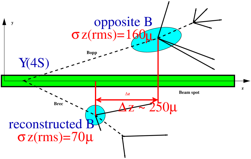
Figure 1: Schematic of lifetime measurements at BaBar (from [12] with added comments).

This is illustrated in Fig. 1. The resolution function is modeled using Monte Carlo simulation.

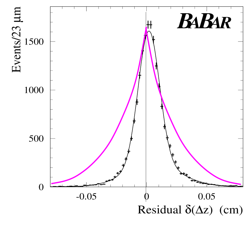
Figure 2: $\Delta z$ Resolution at BaBar for ${\rm B^{+}\to J/\psi K^{+}}$ [12], with $\exp(\Delta z/\mathrm{250\,\mu m})$ superimposed for illustration.

In Fig. 2, the Monte Carlo generated resolution function for $\Delta z$ at BaBar for the decay ${\rm B^{+}\to J/\psi K^{+}}$ is shown [12]. An exponential with a mean decay distance of $\mathrm{250\,mum}$, representing approximately the signal distribution before detector effects, is superimposed, illustrating how the signal is of a similar width as the resolution function, which must therefore be modeled carefully. This modeling of the resolution function, together with the modeling of the background distribution, is the biggest systematic uncertainty in both experiments. The so-called “outliers”, a relatively small number of events with very large reconstructed $\Delta z$, represent a particular problem. Both experiments are able to control it well enough to keep the systematic error below the statistical uncertainty.

Both experiments describe the $\Delta t=\Delta z/\left(c\left(\beta\gamma\right)_{\Upsilon}\right)$ distribution in terms of three components: signal, background and outliers. The beam constrained mass

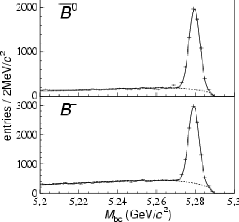
Figure 3: $\mathrm{N^{\underline{o}}}$ of events vs Beam Constrained Mass at Belle [13]

(shown in Fig. 3 for Belle) is used for an event-by-event signal probability. The fraction of outliers is a free fit parameter. The ${\rm B_{d}^{0}}$ and ${\rm B^{+}}$ distributions are fit simultaneously in an unbinned likelihood fit. Besides these commonalities, there are some differences in the event selection and modeling of the resolution function which are described in detail in the publications by the respective experiments [11] [13].

2.2.2 Results

Belle

Using the following fully reconstructed hadronic decays: ${\rm B^{0}\to D^{(*)-}(\pi^{+},\rho^{+}),J/\psi K^{0}_{S},J/\psi K^{*0}}$, ${\rm B^{+}\to\overline{D}^{0}\pi^{+},J/\psi K^{+}}$, Belle find the following ${\rm B_{d}^{0}}$ and ${\rm B^{+}}$ lifetimes [13]:

$$\tau_{{\rm B_{d}^{0}}} = \mathrm{1.554\pm 0.030\pm 0.019\,ps}$$

$$\tau_{{\rm B^{+}}} = \mathrm{1.695\pm 0.026\pm 0.015\,ps}$$

$$\tau_{{\rm B^{+}}}/\tau_{{\rm B_{d}^{0}}} = \mathrm{1.091\pm 0.023\pm 0.014\,}$$

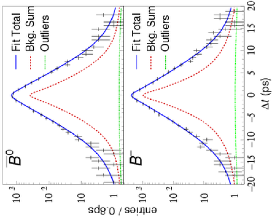
Figure 4: Belle’s life time fit [13].

The fit result to the data, showing separately the background and the outlier contribution, is shown in Fig. 4.

BaBar Fully Hadronic

Using the following fully reconstructed hadronic decays: ${\rm B^{0}\to D^{(*)-}(\pi^{+},\rho^{+},a_{1}^{+}),J/\psi K^{0}_{S},J/\psi K^{*0}}$ and ${\rm B^{+}\to\overline{D}^{0}\pi^{+},J/\psi K^{+},\psi(2S)K^{+}}$ BaBar find the following ${\rm B_{d}^{0}}$ and ${\rm B^{+}}$ lifetimes [11]:

$$\tau_{{\rm B_{d}^{0}}} = \mathrm{1.546\pm 0.032\pm 0.022\,ps}$$

$$\tau_{{\rm B^{+}}} = \mathrm{1.673\pm 0.032\pm 0.023\,ps}$$

$$\tau_{{\rm B^{+}}}/\tau_{{\rm B_{d}^{0}}} = \mathrm{1.082\pm 0.026\pm 0.012\,}$$

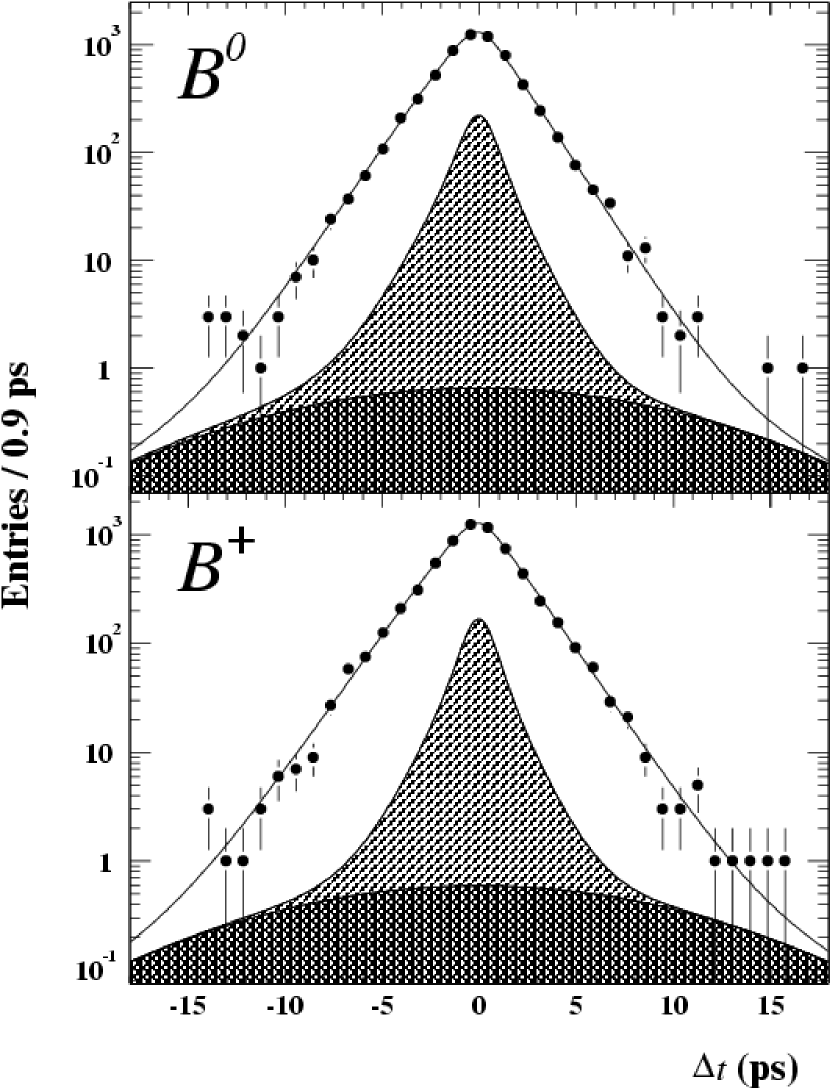
Figure 5: BaBar’s life time fit [11]. Solid line: total fit. Single hatched: total background. Cross hatched: outliers.

The fit result to the data is shown in Fig. 5.

More results from BaBar

As mentioned earlier, the decay kinematics at BaBar and Belle allow to find the $z$ position of a decay vertex from as little as a single track. While in the previously mentioned measurements, one of the pair of B’s is fully reconstructed, BaBar also published a set of measurements where also the ${\rm B_{\mathrm{rec}}}$ is reconstructed partially. These are summarised in Table 1.

	${\rm B^{0}\to D^{*-}\mbox{(}partial)\ell^{+}\nu}$ [14]
$\tau_{{\rm B_{d}^{0}}}$	$\mathrm{1.529\pm 0.012\pm 0.029\,ps}$
	${\rm B^{0}\to D^{*-}\mbox{(}partial)(\pi^{+},\rho^{+})}$ [15]
$\tau_{{\rm B_{d}^{0}}}$	$\mathrm{1.533\pm 0.034\pm 0.038\,ps}$
	${\rm B^{0}\to D^{*-}\ell^{+}\nu}$ [16]
$\tau_{{\rm B_{d}^{0}}}$	$\mathrm{1.523^{+0.024}_{-0.023}\pm 0.022\,ps}$
	Di-lepton (prelim) [17]
$\tau_{{\rm B_{d}^{0}}}$	$\mathrm{1.557\pm 0.028\pm 0.027\,ps}$
$\tau_{{\rm B^{+}}}$	$\mathrm{1.655\pm 0.026\pm 0.027\,ps}$
$\tau_{{\rm B^{+}}}/\tau_{{\rm B_{d}^{0}}}$	$\mathrm{1.064\pm 0.031\pm 0.026\,ps}$

Table 1: BaBar’s results from partially reconstructed decays. Here, a “partial ${\rm D^{*}}$” is a ${\rm D^{*}}$ decaying to to ${\rm D^{0}\pi}$, reconstructed using kinematic constraints and the pion momentum, only, without reconstructing the ${\rm D^{0}}$ [15].

2.2.3 Status of Lifetime Measurements Including Results from BaBar and Belle

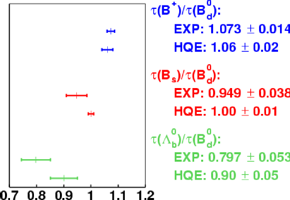
Figure 6: Status of lifetime ratio measurements, incl. results from BaBar, Belle, CDF, LEP. $\tau({\rm B_{s}})/\tau({\rm B_{d}})$ and $\tau({\rm B^{+}})/\tau({\rm B_{d}})$ from [18], $\tau({\rm\Lambda_{b}})/\tau({\rm B_{d}})$ from [19].

Since the B factories have started taking data, they have reduced the error on $\tau_{{\rm B^{+}}}/\tau_{{\rm B_{d}^{0}}}$ by half. Fig. 6 shows the current status of the life time measurements and compares them with HQE predictions. The $\tau_{{\rm B^{+}}}/\tau_{{\rm B_{d}^{0}}}$ measurement, dominated by the precise results from the B factories, is already more precise than that of the HQE prediction, and we can expect further improvements in the near future.

The situation is different for the ${\rm B_{s}}$ and the $\Lambda_{b}$, which are not accessible at the B factories. The experimental precision of the $\tau_{{\rm B_{s}^{0}}}/\tau_{{\rm B_{d}^{0}}}$ measurement lags behind that of the HQE calculations. For the $\Lambda_{b}$, experiment and theory don’t appear to be in very good agreement, but the experimental and theoretical uncertainties are still rather large. Improved measurements and calculations are needed for clarification.

Both, ${\rm B_{s}}$ and ${\rm\Lambda_{b}}$ particles are produced abundantly at hadron colliders, from where we expect dramatically improved lifetime measurements in the near future. The hadron collider currently producing large numbers of ${\rm B_{s}}$ and ${\rm\Lambda_{b}}$ is the Tevatron at Fermilab.

2.3 Lifetimes at the Tevatron

2.3.1 Run II

CDF and DØ have been taking data at Tevatron Run IIa for about two years. For ${\rm p\bar{p}}$ collisions at $\mathrm{1.96\,TeV}$, the $b\overline{b}$ production cross section is $\sigma_{b\overline{b}}\sim\mathrm{0.1\,mb}$.

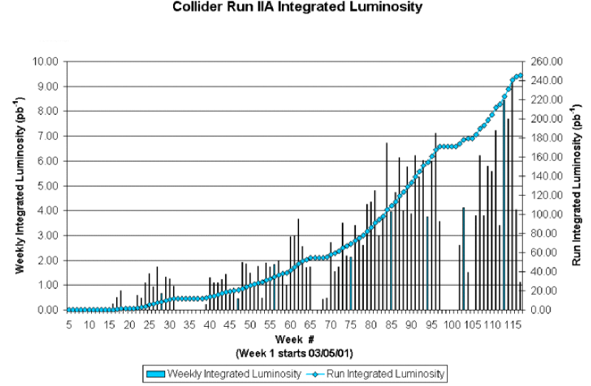
Figure 7: Luminosity at the Tevatron

The integrated luminosity delivered until June 2003 is shown in Fig. 7. The integrated luminosity at Run IIa is expected to be $\mathrm{2\,fb^{-1}}$.

Projected $\int\mathcal{L}dt\;/\;(\mathrm{fb^{-1}})$

Year	Baseline		Stretch
2002	0.	08	0.	08
2003	0.	2	0.	32
2004	0.	4	0.	6
2005	1.	0	1.	5
2006	1.	5	2.	5
2007	1.	5	3.	0
2008	1.	8	3.	0
Total	6.	5	11.

Table 2: Projected integrated luminosity at the Tevatron for baseline and best-case (“stretch”) scenario. The total integrated luminosity by 2008 is expected to be between $\mathrm{6\,fb^{-1}}$ and $\mathrm{11\,fb^{-1}}$.

The projected luminosity for each year until 2008 is listed in Table 2, for two scenarios: The base-line scenario, and a best-case scenario (“stretch”). The total integrated luminosity at the end of Run II in 2008 is expected to lie between $\mathrm{6\,fb^{-1}}$ and $\mathrm{11\,fb^{-1}}$.

2.3.2 DØ and CDF

Both experiments at the Tevatron have undergone major upgrades for Run II, optimising their B physics potential. The most significant upgrade at DØ is the introduction of a magnetic field and a new tracking system providing precise momentum information. This significantly improves the mass resolution. CDF also improved its tracking with a new, faster drift chamber. Both experiments have new Silicon vertex trackers providing excellent proper time resolution, sufficient to resolve the expected fast oscillations in the ${\rm B_{s}^{0}}$ system. The excellent impact parameter resolution is used for triggering on B-events. Both experiments have increased their muon coverage since Run I, and have an efficient di-muon trigger for finding ${\rm B^{0}\to J/\psi X}$ decays. DØ’s $\mu-$trigger covers a particularly large pseudo rapidity range up to $\left|\eta\right|=2$.

IP Trigger

One of the most innovative improvements for B physics at the Tevatron is the large-bandwidth hadron trigger at CDF, which triggers on the impact parameters of tracks at Level 2. The eXtremely Fast Tracker (XFT) uses pattern matching to find tracks in the COT (drift chamber) within $\mathrm{5.5\,\mu s}$, with about $96\%$ efficiency for momenta above $\mathrm{1.5\,GeV}$. These XFT tracks are combined with tracks in the Silicon Vertex Detector by the Silicon Vertex Tracker (SVT), which makes impact parameter information available at Level 2 to a precision of $\mathrm{\sim 50\,\mu m}$. The 2-Track hadron trigger combines the information on the direction (XFT), momentum (XFT) and impact parameter (SVT) to trigger on hadronic B decays.

L1: 2 XFT tracks, $p_{t}>\mathrm{2\,GeV}$, $\Delta\phi<\mathrm{135^{\circ}}$, $p_{t1}+p_{t2}>\mathrm{5.5\,GeV}$. L2: 2-body:
e.g. ${\rm{\rm B_{d}^{0}}\to\pi\pi}$ Multi-body:
e.g. ${\rm{\rm B_{s}^{0}}\to D_{s}\pi}$ $\mathrm{100\,\mu m}<IP<\mathrm{1\,mm}$ $\mathrm{120\,\mu m}<IP<\mathrm{1\,mm}$ $\mathrm{20^{\circ}}<\Delta\phi<\mathrm{135^{\circ}}$ $\mathrm{2^{\circ}}<\Delta\phi<\mathrm{90^{\circ}}$ $L_{xy}$$\mathrm{>200\,\mu m}$ $L_{xy}$$\mathrm{>200\,\mu m}$ IP of B $\mathrm{<140\,\mu m}$ – L3: Same with refined tracks & mass cuts.

Table 3: The CDF hadron trigger. $\Delta\phi$ is the angle between the tracks in the transverse plane. IP is the impact parameter in that plane. $\mathrm{L_{xy}}$ is the decay length in the transverse plane, which can be calculated from the impact parameters and $\Delta\phi$.

The trigger requirements for the two scenarios, 2-body and multi-body B decays, are given in Table 3. The SVT+lepton trigger for semileptonic B decays has impact parameter requirements on one track only and requires additionally an electron or muon with $p_{t}>\mathrm{4\,GeV}$.

DØ also has impact parameter information available at Level 2, and will have a lepton+displaced track trigger, which was however not yet available for the data presented here.

For lifetime measurements it is essential that the bias due to the impact parameter cuts in the trigger is corrected for. We will first consider measurements that do not suffer from such a trigger bias, and then those that do.

2.3.3 Measurements Using Fully Reconstructed Decays, Without IP Trigger

Both experiments have published results from fully reconstructed hadronic ${\rm B\to J/\psi X}$ decays from the dimuon trigger, which are not biased by any impact parameter cut.

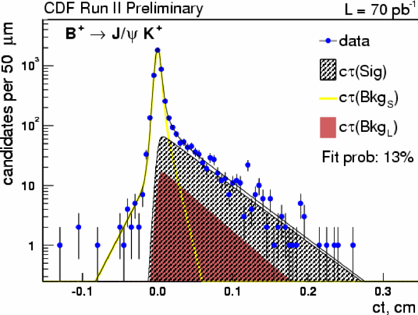
Figure 8: Projection of Fit to $c\tau_{B^{+}}$ from ${\rm B_{u}^{+}\to J/\psi(\mu^{+}\mu^{-})K^{+}}$ at CDF, using $\mathrm{70\,pb^{-1}}$ of data.

An example fit (CDF, $\mathrm{70\,pb^{-1}}$,${\rm B_{u}^{+}\to J/\psi(\mu^{+}\mu^{-})K^{+}}$) is shown in Fig. 8. The signal is modeled with an exponential, the background by a prompt component and two positive and one negative exponential tails (only one positive tail for ${\rm B_{s}^{0}}$ because of lower statistics). Signal and background function are convolved with a single Gaussian to take into account detector effects. The B mass is fit simultaneously and provides an event-by-event signal probability.

Absolute Lifetimes (DØ [20] and CDF [21], Run II prelim.) ${\rm B_{u}^{+}\to J/\psi(\mu^{+}\mu^{-})K^{+}}$ DØ $\mathrm{1.76\pm 0.24(stat)\,ps}$ ${\rm B_{u}^{+}\to J/\psi(\mu^{+}\mu^{-})K^{+}}$ CDF $\mathrm{1.57\pm 0.07\pm 0.02\,ps}$ ${\rm B_{d}^{0}\to J/\psi(\mu^{+}\mu^{-})K^{*0}}$ CDF $\mathrm{1.42\pm 0.09\pm 0.02\,ps}$ ${\rm B_{s}^{0}\to J/\psi(\mu^{+}\mu^{-})\phi}$ CDF $\mathrm{1.26\pm 0.20\pm 0.02\,ps}$ Lifetime Ratios (CDF [21], Run II prelim., compared with world average (ave) [18] and HQE predictions [5]):

Table 4: Lifetimes from ${\rm B\to J/\psi X}$ at Tevatron Run II. CDF data correspond to an integrated luminosity of $\mathrm{70\,pb^{-1}}$.

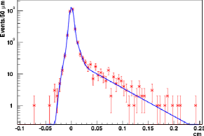
Sidebands	Mass ($\mathrm{L_{xy}>400\,\mu m}$)
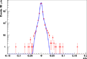
left sideband: right sideband	(Mass resolution has improved by factor $\sim 2$ since this plot was produced)
Signal Region:

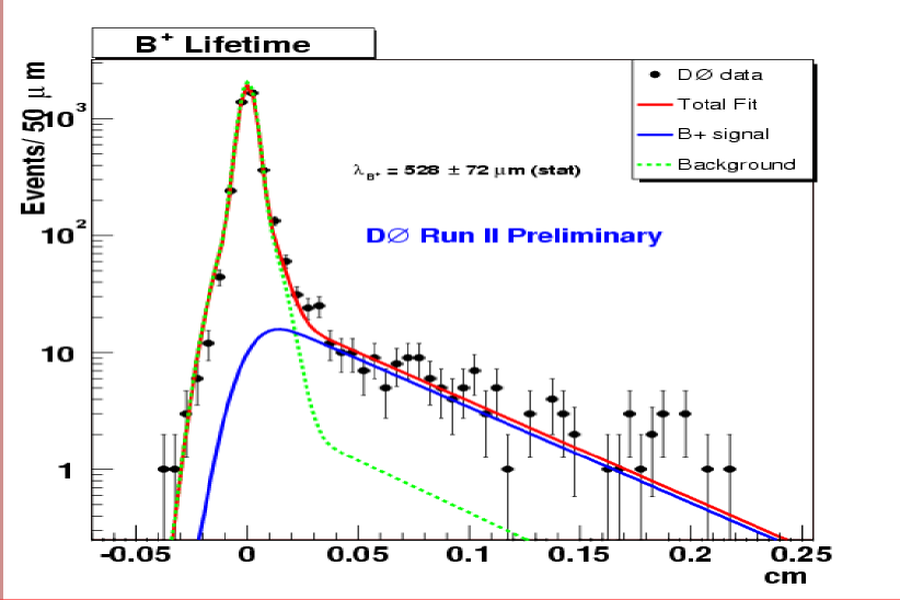
Figure 9: Life time fit at DØ

DØ use a somewhat different approach, as illustrated in Fig. 9, modeling the background using a separate fit to the right sideband. The left sideband has a long-lifetime component from incompletely reconstructed other B decays. This B contamination in the signal region is modeled from Monte Carlo and found to be $12\%$.

The results are given in Table 4. The table shows that the error on the life time ratios obtained from ${\rm B\to J/\psi X}$ decays is about twice that achieved in Run I, all channels combined. By the end of this year, CDF is expected to have collected $\mathrm{\sim 300\,pb^{-1}}$, four times as much as used for the analyses presented here, so we can expect CDF to achieve the combined Run I precision using the exclusive channels alone by the end of this year.

2.3.4 Measurements Using Partially Reconstructed Decays, Without IP Trigger

Inclusive $\tau_{B}$

Since all B hadrons can decay to ${\rm J/\psi}$, reconstructing ${\rm J/\psi}$ vertices allows to find an average B lifetime, where the composition of the sample depends on the detector and selection criteria. Since the decay is not fully reconstructed, the momentum of the B, which is needed to calculate the proper lifetime from $\tau(B)=L_{xy}M(B)/(cp_{t}(B))$ is unknown. It can however be related to the ${\rm J/\psi}$ momentum via

$$p_{t}\left(B\right)=F\left(p_{t}\left(J/\psi\right)\right)\cdot p_{t}\left(J/\psi\right)$$

where $F\left(p_{t}\left(J/\psi\right)\right)$ is the mean ratio $p_{t}\left(B\right)/p_{t}\left(J/\psi\right)$, and the uncertainty on $p_{t}\left(B\right)$ depends on the the spread of that ratio for different momenta. Both the mean ratio and its variance are obtained from Monte Carlo.

$\frac{p_{t}(B)}{p_{t}({\rm J/\psi})}$       

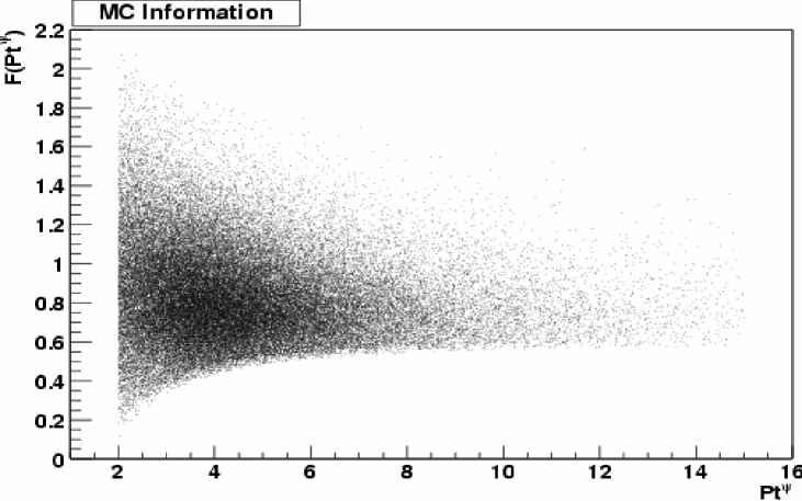
$p_{t}({\rm J/\psi})$

$F=\left<\frac{p_{t}(B)}{p_{t}({\rm J/\psi})}\right>$      

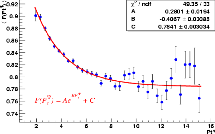
$p_{t}({\rm J/\psi})$

Figure 10: The F-factor (DØ)

The results of such a Monte Carlo study at DØ are shown in Fig. 10. The measured average B-hadron lifetimes are

• DØ (March 03): $\tau_{B}=\mathrm{1.561\pm 0.024\pm 0.074\,ps}$

• CDF (July 02): $\tau_{B}=\mathrm{1.526\pm 0.034\pm 0.035\,ps}$

which is consistent with the world average of $\mathrm{\tau_{B}=1.573\pm 0.007\,ps}$ [18].

2.3.5 Semileptonic Decays With $\ell+$ IP Trigger

CDF is also using ${\rm B\to D\ell\nu\;X}$ and ${\rm\Lambda_{b}\to\Lambda_{c}\ell\nu}$ decays from the lepton plus displaced track trigger for lifetime measurements. The missing $\nu$ momentum is accounted for using the same Monte Carlo-based method as in the inclusive B lifetime study discussed above. The main challenge is to correct the lifetime bias due to the impact parameter cuts in the trigger. The acceptance as a function of lifetime

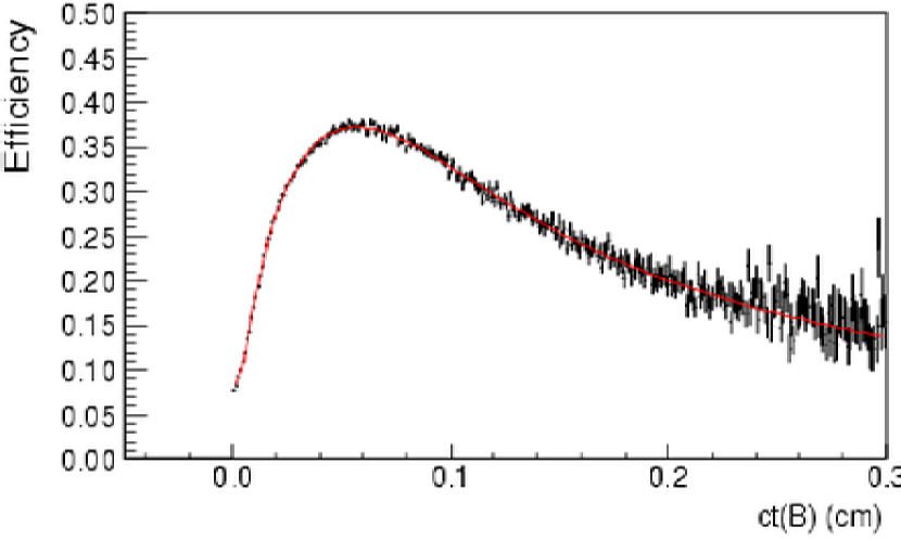
Figure 11: SVT acceptance as a function of $c\tau_{B}$ (CDF)

shown in Fig. 11 is found by a detailed Monte Carlo study. A fit to the ${\rm B_{s}\to D_{s}\mu\nu}$

Sideband                               Signal

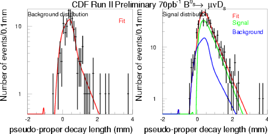
Figure 12: Fit to lifetime distribution from ${\rm B_{s}\to D_{s}\mu\nu}$

life time distribution is shown in Fig. 12. The statistical precision achieved with the current data sample is $\sigma_{\tau_{B^{+}}}=\mathrm{\sim 0.05\,ps}$, $\sigma_{\tau_{B^{0}_{d}}}=\mathrm{\sim 0.06\,ps}$, $\sigma_{\tau_{B_{s}}}=\mathrm{\sim 0.10\,ps}$, $\sigma_{\tau_{\Lambda_{b}}}=\mathrm{\sim 0.13\,ps}$. The full results will be published as soon as the systematic errors are fully understood.

2.3.6 Lifetimes at the Tevatron - Summary & Prospects

The Tevatron is going to provide high statistics samples of all B-hadrons, including ${\rm B_{s},B_{c},\Lambda_{b}}$. Preliminary Run II results from fully reconstructed hadronic decays are already approaching Run I precision, higher statistical precision is expected soon from the lepton+displaced track sample. The Run IIa projection (MC studies from Dec-01 [3]) for the life time ratios are

• $\sigma(\tau_{{\rm B_{s}}}/\tau_{{\rm B^{0}_{d}}})$, $\sigma(\tau_{{\rm\Lambda_{b}}}/\tau_{{\rm B^{0}_{d}}})<1\%$

which will provide a real test of theory for the ${\rm B_{s}}$ and, pending improved theoretical calculations, for the ${\rm\Lambda_{b}}$ lifetime.

3 Lifetime Differences

3.1 Introduction

The width difference between long and short lived CP eigenstates of the ${\rm B_{s,d}^{0}-\bar{B}_{s,d}^{0}}$ system is predicted to be

• $\frac{\Delta\Gamma_{s}}{\Gamma_{s}}\sim\mathcal{O}(10)\%$

• $\frac{\Delta\Gamma_{d}}{\Gamma_{d}}\sim\mathcal{O}(1\%)$

$\frac{\Delta\Gamma_{s}}{\Gamma_{s}}$ is large enough to be experimentally accessible, soon. The width difference is directly proportional to the mass difference,

$$\Delta\Gamma_{s}=A\cdot\Delta m_{s}.$$

where the proportionality constant $A$ is $\sim 3\cdot 10^{-3}$ in the Standard Model, but the value suffers from large hadronic uncertainties [10]. The mass difference $\Delta m_{s}$, accessible through the oscillation frequency in the ${\rm B_{s}^{0}}$ system, is itself an unknown parameter of great interest, and a major motivation for installing the precise vertex detectors at CDF and DØ during their upgrades for Run II. It is interesting to note that a large value for $\Delta m_{s}$, corresponding to fast ${\rm B_{s}^{0}}$ oscillations which are more difficult to measure, corresponds to a large value for $\Delta\Gamma_{s}$, which makes it easier to measure. $\Delta\Gamma_{s}$ and $\Delta m_{s}$ are complementary measurements. Given the current limits on $\Delta m_{s}$, a very small value for $\Delta\Gamma_{s}$ would be a hint at new physics.

Theory Status

Recent theoretical predictions for $\Delta\Gamma_{d}$ are (the different results are obtained using different expansions of Next-To-Leading Order QCD corrections:

• $\frac{\Delta\Gamma_{d}}{\Gamma_{d}}=\left(2.6^{+1.2}_{-1.6}\right)\cdot 10^{-3}$ [9]

• $\frac{\Delta\Gamma_{d}}{\Gamma_{d}}=\left(3.0^{+0.9}_{-1.4}\right)\cdot 10^{-3}$ [9] using method in [3]

For $\Delta\Gamma_{s}$, recent predictions are:

• $\frac{\Delta\Gamma_{s}}{\Gamma_{s}}=\left(8.5\pm 2.8\right)\%$ [5] using method in [10]

• $\frac{\Delta\Gamma_{s}}{\Gamma_{s}}=\left(9.0\pm 2.8\right)\%$ [5] using method in [7]

3.2 Strategies for Extracting $\Delta\Gamma_{s}$

In principle, one could simply fit two exponentials to the lifetime distribution of ${\rm B_{s}^{0}}$ decays to mixed CP states. However, since $\frac{\Delta\Gamma_{s}}{\Gamma_{s}}\sim\mathcal{O}(10\%)$ only, this method would require very high statistics, therefore extra information is needed to seperate the CP eigenstates. Possible strategies include [3]:

• Fit lifetime to purely CP-even ${\rm{\rm B_{s}^{0}}\to D_{s}D_{s}}$. With certain assumptions ${\rm{\rm B_{s}^{0}}\to D^{(*)}_{s}D^{*}_{s}}$ is predicted to be mostly CP even, so that these decays could be included in the analysis. These assumption would have to be tested however, for example with a similar angular analysis as for the ${\rm{\rm B_{s}^{0}}\to J/\psi\phi}$ case. The result for the CP even life time can then be compared to the mean lifetime from CP-mixed channels to extract the lifetime difference.

• Fit 2 lifetimes to ${\rm{\rm B_{s}^{0}}\to J/\psi\phi}$. This can have 3 angular momentum states, 2 CP even, 1 CP odd. These can be disantangled by an angular analysis.

• The B.R. Method: Assume that the width difference is entirely due to CP-even ${\rm{\rm B_{s}^{0}}\to D^{(*)}_{s}D^{(*)}_{s}}$. In small velocity (Shifman-Voloshin) limit [3], [22]:

  $$BR({\rm{\rm B_{s}^{0}}\to D^{(*)}_{s}D^{(*)}_{s}})=\frac{\Delta\Gamma_{s}/\Gamma_{s}}{1+\frac{1}{2}\Delta\Gamma_{s}/\Gamma_{s}}$$

3.3 Current Values for $\Delta\Gamma$

Recent results for the width differences in the B system are

• $\frac{\Delta\Gamma_{d}}{\Gamma_{d}}<0.18$ (95% CL) (DELPHI, 2002) [23]

• $\frac{\Delta\Gamma_{s}}{\Gamma_{s}}<0.31$ (95% CL) (combined LEP, CDF, for $1/\Gamma_{s}=\tau({\rm B_{d}^{0}})$, using lifetime method) [18]

• $\frac{\Delta\Gamma_{s}}{\Gamma_{s}}=0.26^{+0.30}_{-0.15}$ (ALEPH, from B.R. method) [22]

3.4 Prospects for $\Delta\Gamma$ at the Tevatron

CDF expects the following precisions on $\Delta\Gamma_{s}$ by the end of Run IIa, from $\mathrm{2\,fb^{-1}}$. The projections assume $\frac{\Delta\Gamma_{s}}{\Gamma_{s}}=15\%$ and are those given in [3] in December 2001. They refer to the statistical error only.

• From ${\rm B_{s}\to J/\psi\phi}$: $\sigma_{\mathrm{stat}}(\frac{\Delta\Gamma_{s}}{\Gamma_{s}})\sim 5\%$

• ${\rm B_{s}\to D_{s}D_{s}}$ (no ${\rm D_{s}^{*}}$): $\sigma_{\mathrm{stat}}(\frac{\Delta\Gamma_{s}}{\Gamma_{s}})\sim 6\%$

• ${\rm B_{s}\to D_{s}^{(*)}D_{s}^{(*)}}$: $\sigma_{\mathrm{stat}}(\frac{\Delta\Gamma_{s}}{\Gamma_{s}})\sim 2.5\%$
  (assume decay 100% CP even)

• B.R. method: $\sigma_{\mathrm{stat}}(\frac{\Delta\Gamma_{s}}{\Gamma_{s}})\sim 1\%$
  (model dependent)

Assuming a similar performance for ${\rm B_{s}\to J/\psi\phi}$ at DØ we arrive at a total statistical uncertainty at the Tevatron for $\mathrm{2\,fb^{-1}}$ of $\sigma_{\mathrm{stat}}(\frac{\Delta\Gamma_{s}}{\Gamma_{s}})\sim 2\%$, ignoring the B.R. method. A more conservative estimate of $\sigma_{\mathrm{stat}}(\frac{\Delta\Gamma_{s}}{\Gamma_{s}})\sim 3\%$ is obtained if the assumption that ${\rm B_{s}\to D_{s}^{(*)}D_{s}^{*}}$ decays are 100% CP even is dropped and decays involving ${\rm D_{s}^{*}}$ are completely ignored.

4 Conclusion

Lifetime ratios

Since they have started data taking, the B-factories have brought the error on $\sigma(\tau_{{\rm B^{+}}}/\tau_{{\rm B^{0}_{d}}})$ down to $1.7\%$, so that the experimental accuracy for this ratio is now better than that of the HQE prediction. The agreement between theory and experiment is very good. Further improvements on $\sigma(\tau_{{\rm B^{+}}}/\tau_{{\rm B^{0}_{d}}})$ can be expected from B-factories and Tevatron, soon.

Large numbers of ${\rm B_{s}^{0}}$ and ${\rm\Lambda_{b}}$ are currently being produced at the Tevatron. The uncertainty on the lifetime ratios $\sigma(\tau_{{\rm B_{s}}}/\tau_{{\rm B^{0}_{d}}})$, $\sigma(\tau_{{\rm\Lambda_{b}}}/\tau_{{\rm B^{0}_{d}}})$ is expected to be below $1\%$ by the end of Run IIa. This will provide a real test of HQE for ${\rm B_{s}}$ for which precise predictions exist, while improved theoretical values are needed for for ${\rm\Lambda_{b}}$.

Lifetime Differences

$\Delta\Gamma_{s}$ and $\Delta m_{s}$ are complementary measurements, and both parameters combined are sensitive to New Physics contributions to ${\rm B_{s}^{0}}$ mixing. Recent calculations predict $\frac{\Delta\Gamma_{s}}{\Gamma_{s}}=9\pm 3\%$ [5].

From data we get the following limit on the lifetime difference in the ${\rm B_{s}}$ system: $\frac{\Delta\Gamma_{s}}{\Gamma_{s}}<0.31$ (95% CL) [18]. First steps have been taken towards a $\frac{\Delta\Gamma_{s}}{\Gamma_{s}}$ measurement at the Tevatron, where $55\pm 9$ ${\rm B_{s}\to J/\psi\phi}$ events have been reconstructed at CDF, and an average ${\rm B_{s}}$ lifetime has been extracted from that decay. By the end of Run IIa a measurement of $\frac{\Delta\Gamma_{s}}{\Gamma_{s}}$ with a statistical uncertainty of $\sim 2\%$ is expected.

References

- [1] N. Uraltsev, arXiv:hep-ph/9804275.
- [2] M. A. Shifman, arXiv:hep-ph/0009131.
- [3] K. Anikeev et al., arXiv:hep-ph/0201071.
- [4] E. Franco, V. Lubicz, F. Mescia and C. Tarantino, Nucl. Phys. B 633 (2002) 212 arXiv:hep-ph/0203089.
- [5] M Battaglia, AJ Buras, P Gambino and A Stocchi, eds. Proceedings of the First Workshop on the CKM Unitarity Triangle, CERN, Feb 2002, arXiv:hep-ph/0304132
- [6] M. Beneke and A. Lenz, J. Phys. G 27 (2001) 1219
- [7] D. Becirevic, D. Meloni, A. Retico, V. Gimenez, V. Lubicz and G. Martinelli, Eur. Phys. J. C 18 (2000) 157 [arXiv:hep-ph/0006135].
- [8] T. Hurth et al., J. Phys. G 27 (2001) 1277 [arXiv:hep-ph/0102159].
- [9] A. S. Dighe, T. Hurth, C. S. Kim and T. Yoshikawa, Nucl. Phys. B 624 (2002) 377 [arXiv:hep-ph/0109088]. .
- [10] M. Beneke, G. Buchalla, C. Greub, A. Lenz and U. Nierste, Phys. Lett. B 459 (1999) 631 [arXiv:hep-ph/9808385].
- [11] B. Aubert et al. [BABAR Collaboration], Phys. Rev. Lett. 87 (2001) 201803 [arXiv:hep-ex/0107019].
- [12] B. Aubert et al. [BABAR Collaboration], Aug 2000, SLAC-PUB-8529 [arXiv:hep-ex/0008060].
- [13] K. Abe et al. [BELLE Collaboration], Phys. Rev. Lett. 88 (2002) 171801 [arXiv:hep-ex/0202009].
- [14] B. Aubert et al. [BABAR Collaboration], Phys. Rev. Lett. 89 (2002) 011802 [Erratum-ibid. 89 (2002) 169903] [arXiv:hep-ex/0202005].
- [15] B. Aubert et al. [BABAR Collaboration], Phys. Rev. D 67 (2003) 091101 [arXiv:hep-ex/0212012].
- [16] B. Aubert et al. [BABAR Collaboration], Phys. Rev. D 67 (2003) 072002 [arXiv:hep-ex/0212017].
- [17] Daniele de Re , May 2002, BABAR-TALK-02034
-
[18]
Heavy Flavour Averaging Group.
Method:
D. Abbaneo et al. [ALEPH, CDF, DELPHI, L3, OPAL, SLD], June 2001, CERN-EP/2001-050, arXiv:hep-ex/0112028. Results March 2003:
http://lepbosc.web.cern.ch/LEPBOSC/
combined_results/lathuile_2003 - [19] K. Hagiwara et al., Phys. Rev. D 66, 010001 (2002)
-
[20]
Pedro Podesta
March 2003,
http://www-d0.fnal.gov/
podesta/BplusLifetime_Report.ps - [21] K.Anikeev, G.Bauer, Ch.Paus March 2003, CDF/DOC/BOTTOM/CDFR/6266
- [22] R. Barate et al. [ALEPH Collaboration], Phys. Lett. B 486 (2000) 286.
- [23] J. Abdallah et al. [DELPHI Collaboration], Eur. Phys. J. C 28 (2003) 155 [arXiv:hep-ex/0303032].