EUROPEAN ORGANIZATION FOR NUCLEAR RESEARCH (CERN)

CERN-EP 2003-025

May, 20 2003

Study of hadronic final states from
double tagged $\gamma\gamma$ events at LEP

The ALEPH Collaboration^∗)

The interaction of virtual photons is investigated using double tagged $\gamma\gamma$ events with hadronic final states recorded by the ALEPH experiment at $\mathrm{e}^{+}\mathrm{e}^{-}$ centre-of-mass energies between $188$ and $209\,\mathrm{GeV}$. The measured cross section is compared to Monte Carlo models, and to next-to-leading-order QCD and BFKL calculations.

Submitted to The European Physical Journal C

${}^{*})$ See next pages for the list of authors

The ALEPH Collaboration

A. Heister, S. Schael

Physikalisches Institut das RWTH-Aachen, D-52056 Aachen, Germany

R. Barate, R. Brunelière, I. De Bonis, D. Decamp, C. Goy, S. Jezequel, J.-P. Lees, F. Martin, E. Merle, M.-N. Minard, B. Pietrzyk, B. Trocmé

Laboratoire de Physique des Particules (LAPP), IN²P³-CNRS, F-74019 Annecy-le-Vieux Cedex, France

S. Bravo, M.P. Casado, M. Chmeissani, J.M. Crespo, E. Fernandez, M. Fernandez-Bosman, Ll. Garrido,¹⁵ M. Martinez, A. Pacheco, H. Ruiz

Institut de Física d’Altes Energies, Universitat Autònoma de Barcelona, E-08193 Bellaterra (Barcelona), Spain⁷

A. Colaleo, D. Creanza, N. De Filippis, M. de Palma, G. Iaselli, G. Maggi, M. Maggi, S. Nuzzo, A. Ranieri, G. Raso,²⁴ F. Ruggieri, G. Selvaggi, L. Silvestris, P. Tempesta, A. Tricomi,³ G. Zito

Dipartimento di Fisica, INFN Sezione di Bari, I-70126 Bari, Italy

X. Huang, J. Lin, Q. Ouyang, T. Wang, Y. Xie, R. Xu, S. Xue, J. Zhang, L. Zhang, W. Zhao

Institute of High Energy Physics, Academia Sinica, Beijing, The People’s Republic of China⁸

D. Abbaneo, T. Barklow,²⁶ O. Buchmüller,²⁶ M. Cattaneo, B. Clerbaux,²³ H. Drevermann, R.W. Forty, M. Frank, F. Gianotti, J.B. Hansen, J. Harvey, D.E. Hutchcroft,³⁰, P. Janot, B. Jost, M. Kado,² P. Mato, A. Moutoussi, F. Ranjard, L. Rolandi, D. Schlatter, G. Sguazzoni, W. Tejessy, F. Teubert, A. Valassi, I. Videau

European Laboratory for Particle Physics (CERN), CH-1211 Geneva 23, Switzerland

F. Badaud, S. Dessagne, A. Falvard,²⁰ D. Fayolle, P. Gay, J. Jousset, B. Michel, S. Monteil, D. Pallin, J.M. Pascolo, P. Perret

Laboratoire de Physique Corpusculaire, Université Blaise Pascal, IN²P³-CNRS, Clermont-Ferrand, F-63177 Aubière, France

J.D. Hansen, J.R. Hansen, P.H. Hansen, A.C. Kraan, B.S. Nilsson

Niels Bohr Institute, 2100 Copenhagen, DK-Denmark⁹

A. Kyriakis, C. Markou, E. Simopoulou, A. Vayaki, K. Zachariadou

Nuclear Research Center Demokritos (NRCD), GR-15310 Attiki, Greece

A. Blondel,¹² J.-C. Brient, F. Machefert, A. Rougé, M. Swynghedauw, R. Tanaka H. Videau

Laoratoire Leprince-Ringuet, Ecole Polytechnique, IN²P³-CNRS, F-91128 Palaiseau Cedex, France

V. Ciulli, E. Focardi, G. Parrini

Dipartimento di Fisica, Università di Firenze, INFN Sezione di Firenze, I-50125 Firenze, Italy

A. Antonelli, M. Antonelli, G. Bencivenni, F. Bossi, G. Capon, F. Cerutti, V. Chiarella, P. Laurelli, G. Mannocchi,⁵ G.P. Murtas, L. Passalacqua

Laboratori Nazionali dell’INFN (LNF-INFN), I-00044 Frascati, Italy

J. Kennedy, J.G. Lynch, P. Negus, V. O’Shea, A.S. Thompson

Department of Physics and Astronomy, University of Glasgow, Glasgow G12 8QQ,United Kingdom¹⁰

S. Wasserbaech

Utah Valley State College, Orem, UT 84058, U.S.A.

R. Cavanaugh,⁴ S. Dhamotharan,²¹ C. Geweniger, P. Hanke, V. Hepp, E.E. Kluge, A. Putzer, H. Stenzel, K. Tittel, M. Wunsch¹⁹

Kirchhoff-Institut für Physik, Universität Heidelberg, D-69120 Heidelberg, Germany¹⁶

R. Beuselinck, W. Cameron, G. Davies, P.J. Dornan, M. Girone,¹ R.D. Hill, N. Marinelli, J. Nowell, S.A. Rutherford, J.K. Sedgbeer, J.C. Thompson,¹⁴ R. White

Department of Physics, Imperial College, London SW7 2BZ, United Kingdom¹⁰

V.M. Ghete, P. Girtler, E. Kneringer, D. Kuhn, G. Rudolph

Institut für Experimentalphysik, Universität Innsbruck, A-6020 Innsbruck, Austria¹⁸

E. Bouhova-Thacker, C.K. Bowdery, D.P. Clarke, G. Ellis, A.J. Finch, F. Foster, G. Hughes, R.W.L. Jones, M.R. Pearson, N.A. Robertson, M. Smizanska

Department of Physics, University of Lancaster, Lancaster LA1 4YB, United Kingdom¹⁰

O. van der Aa, C. Delaere,²⁸ G.Leibenguth,³¹ V. Lemaitre²⁹

Institut de Physique Nucléaire, Département de Physique, Université Catholique de Louvain, 1348 Louvain-la-Neuve, Belgium

U. Blumenschein, F. Hölldorfer, K. Jakobs, F. Kayser, K. Kleinknecht, A.-S. Müller, B. Renk, H.-G. Sander, S. Schmeling, H. Wachsmuth, C. Zeitnitz, T. Ziegler

Institut für Physik, Universität Mainz, D-55099 Mainz, Germany¹⁶

A. Bonissent, P. Coyle, C. Curtil, A. Ealet, D. Fouchez, P. Payre, A. Tilquin

Centre de Physique des Particules de Marseille, Univ Méditerranée, IN²P³-CNRS, F-13288 Marseille, France

F. Ragusa

Dipartimento di Fisica, Università di Milano e INFN Sezione di Milano, I-20133 Milano, Italy.

A. David, H. Dietl, G. Ganis,²⁷ K. Hüttmann, G. Lütjens, W. Männer, H.-G. Moser, R. Settles, M. Villegas, G. Wolf

Max-Planck-Institut für Physik, Werner-Heisenberg-Institut, D-80805 München, Germany

J. Boucrot, O. Callot, M. Davier, L. Duflot, J.-F. Grivaz, Ph. Heusse, A. Jacholkowska,⁶ L. Serin, J.-J. Veillet

Laboratoire de l’Accélérateur Linéaire, Université de Paris-Sud, IN²P³-CNRS, F-91898 Orsay Cedex, France

P. Azzurri, G. Bagliesi, T. Boccali, L. Foà, A. Giammanco, A. Giassi, F. Ligabue, A. Messineo, F. Palla, G. Sanguinetti, A. Sciabà, P. Spagnolo R. Tenchini A. Venturi P.G. Verdini

Dipartimento di Fisica dell’Università, INFN Sezione di Pisa, e Scuola Normale Superiore, I-56010 Pisa, Italy

O. Awunor, G.A. Blair, G. Cowan, A. Garcia-Bellido, M.G. Green, L.T. Jones, T. Medcalf, A. Misiejuk, J.A. Strong, P. Teixeira-Dias

Department of Physics, Royal Holloway & Bedford New College, University of London, Egham, Surrey TW20 OEX, United Kingdom¹⁰

R.W. Clifft, T.R. Edgecock, P.R. Norton, I.R. Tomalin, J.J. Ward

Particle Physics Dept., Rutherford Appleton Laboratory, Chilton, Didcot, Oxon OX11 OQX, United Kingdom¹⁰

B. Bloch-Devaux, D. Boumediene, P. Colas, B. Fabbro, E. Lançon, M.-C. Lemaire, E. Locci, P. Perez, J. Rander, B. Tuchming, B. Vallage

CEA, DAPNIA/Service de Physique des Particules, CE-Saclay, F-91191 Gif-sur-Yvette Cedex, France¹⁷

N. Konstantinidis, A.M. Litke, G. Taylor

Institute for Particle Physics, University of California at Santa Cruz, Santa Cruz, CA 95064, USA²²

C.N. Booth, S. Cartwright, F. Combley,²⁵ P.N. Hodgson, M. Lehto, L.F. Thompson

Department of Physics, University of Sheffield, Sheffield S3 7RH, United Kingdom¹⁰

A. Böhrer, S. Brandt, C. Grupen, J. Hess, A. Ngac, G. Prange

Fachbereich Physik, Universität Siegen, D-57068 Siegen, Germany¹⁶

C. Borean, G. Giannini

Dipartimento di Fisica, Università di Trieste e INFN Sezione di Trieste, I-34127 Trieste, Italy

H. He, J. Putz, J. Rothberg

Experimental Elementary Particle Physics, University of Washington, Seattle, WA 98195 U.S.A.

S.R. Armstrong, K. Berkelman, K. Cranmer, D.P.S. Ferguson, Y. Gao,¹³ S. González, O.J. Hayes, H. Hu, S. Jin, J. Kile, P.A. McNamara III, J. Nielsen, Y.B. Pan, J.H. von Wimmersperg-Toeller, W. Wiedenmann, J. Wu, Sau Lan Wu, X. Wu, G. Zobernig

Department of Physics, University of Wisconsin, Madison, WI 53706, USA¹¹

G. Dissertori

Institute for Particle Physics, ETH Hönggerberg, 8093 Zürich, Switzerland.

1 Introduction

The largest part of the cross section for inelastic processes at LEP2 is due to two-photon scattering. Interactions of two photons can be studied at $\mathrm{e}^{+}\mathrm{e}^{-}$ colliders by investigating the reaction

$$\mathrm{e}^{+}\mathrm{e}^{-}\rightarrow\mathrm{e}^{+}\mathrm{e}^{-}\gamma\gamma\rightarrow\mathrm{e}^{+}\mathrm{e}^{-}\mathrm{X}$$ (1)

where the photons can be quasi-real or virtual and the hadronic final state is denoted by X.

The analysis reported in this paper focusses on the interactions of virtual photons by selecting only double tagged events, i.e., events where both scattered electrons are detected. Here, electrons and positrons are generically referred to as electrons. Differential cross sections for this process are measured as a function of several kinematic variables and presented here.

The purpose of this paper is to compare the measured differential cross sections with the predictions of the PYTHIA [1] and PHOT02 [2] Monte Carlo generators, with a next-to-leading-order (NLO) QCD calculation [3] and with BFKL calculations [4, 5, 6, 7, 8].

2 Theoretical Framework

Interactions of virtual photons can be studied by requiring that both electrons be detected after radiating the photons. The kinematics of these electron-induced $\gamma\gamma$ interactions is sketched in Fig. 1. The symbols in parentheses represent the four-momenta of the particles.

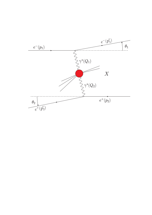
Figure 1: Kinematics of $\gamma\gamma$ interactions at an $\mathrm{e^{+}e^{-}}$ collider

The kinematics can be described by the dimensionless Björken variables of deep inelastic scattering:

$$x_{i} = \frac{Q_{i}^{2}}{Q^{2}_{1}+Q^{2}_{2}+W^{2}_{\gamma\gamma}}\quad,$$ (2)

$$y_{i} = 1-\frac{E_{i}^{\prime}}{E_{\mathrm{beam}}}\cos^{2}\left(\frac{\theta_{i}}{2}\right),$$ (3)

where $i=1,2$ refers to the scattered electron, positron. The hadronic invariant mass $W_{\gamma\gamma}$ used in these definitions is obtained from the energies $E_{h}$ and the momenta $\vec{p}_{h}$ of the final state particles $h$ by

$$W_{\gamma\gamma}^{2}=\left(\sum_{h}E_{h}\right)^{2}-\left(\sum_{h}\vec{p}_{h}\right)^{2}=E^{2}_{\mathrm{X}}-\vec{p}^{\;2}_{\mathrm{X}}\ .$$ (4)

The virtualities of the photons $Q^{2}_{i}$ are

$$Q_{i}^{2}=-(p_{i}-p_{i}^{\prime})^{2}=2E_{\mathrm{beam}}E_{i}^{\prime}(1-\cos\theta_{i})$$ (5)

for $\theta_{i}\gg m_{\mathrm{electron}}/E_{i}$, where $\theta_{i}$ are the scattering angles of the deflected leptons.

From Eq. (5) it is possible to select interactions of virtual photons by requiring that the scattered electrons be detected at large angles. The accessible range of virtualities and therefore the phase space depends on the region where electrons can be detected.

For the comparison of the data with BFKL calculations the following quantity is defined,

$$Y=\log{\left(\frac{s}{s_{0}}\right)}\ ,$$ (6)

where $\sqrt{s}$ is the LEP centre-of-mass energy and $s/s_{0}=sy_{1}y_{2}/\sqrt{Q^{2}_{1}Q^{2}_{2}}\approx W^{2}_{\gamma\gamma}/\sqrt{Q^{2}_{1}Q^{2}_{2}}$, the approximation requiring $W^{2}_{\gamma\gamma}\gg Q^{2}_{i}$.

To correct the data for detector effects, the signal Monte Carlo simulation for this analysis uses PYTHIA 6.151 [1, 9, 10] and as an alternative PHOT02 [2]. The PHOJET generator [11], which simulates untagged events, gives information for further systematic studies.

The PHOT02 generator is a combination of different two-photon generators. The main contribution to this analysis comes from the QED part, based on a program that gives a matrix element calculation for $\mathrm{e}^{+}\mathrm{e}^{-}\rightarrow\mathrm{e}^{+}\mathrm{e}^{-}\ell^{+}\ell^{-}$, where $\ell^{\pm}$ are charged fermions [12, 13, 14]. A small contribution arises from the vector-meson dominance model (VDM) [15, 16]. The implementation of the $\gamma\gamma$ generator in PYTHIA is based on a model described in [9, 10].

The background from leptonic double tagged two-photon events is also simulated with PHOT02. For annihilation events three generators are employed: KORALZ [17], PYTHIA and HERWIG [18]. The latter is used to generate single tagged two-photon events contributing to the background.

3 ALEPH Detector

A detailed description of the ALEPH detector and its performance can be found in Ref. [19]. The inner part of the ALEPH detector is dedicated to the reconstruction of the trajectories of charged particles with a two-layer silicon strip vertex detector (VDET), a cylindrical drift chamber (ITC) and a large time projection chamber (TPC). The three tracking detectors are immersed in a $1.5\,{\mathrm{T}}$ axial magnetic field provided by a superconducting solenoidal coil. Together they measure charged particle momenta with a resolution of $\delta p_{\mathrm{t}}/p_{\mathrm{t}}=6\times 10^{-4}p_{\mathrm{t}}\oplus 0.005$ ($p_{\mathrm{t}}$ in GeV/$c$).

Photons are identified in the electromagnetic calorimeter (ECAL), situated between the TPC and the coil. The ECAL is a lead/proportional-tube sampling calorimeter segmented into $0.9^{\circ}\times 0.9^{\circ}$ projective towers read out in three sections in depth. It has a total thickness of 22 radiation lengths and yields a relative energy resolution of $0.18/\sqrt{E}+0.009$ ($E$ in GeV) for isolated photons. Electrons crossing the TPC are identified by their transverse and longitudinal shower profiles in ECAL and their specific ionization in the TPC.

The iron return yoke is instrumented with 23 layers of streamer tubes and forms the hadron calorimeter (HCAL). The latter provides a relative energy resolution for charged and neutral hadrons of $0.85/\sqrt{E}$ ($E$ in GeV). Muons are distinguished from hadrons by their characteristic pattern in HCAL and by the muon chambers, which are composed of two double-layers of streamer tubes outside HCAL.

The information from the tracking detectors and the calorimeters are combined in an energy-flow algorithm [19]. For each event, the algorithm provides a set of charged and neutral reconstructed particles, called energy-flow objects.

Two small-angle luminosity calorimeters, the silicon luminosity calorimeter (SICAL) and the luminosity calorimeter (LCAL), are used to detect and measure the energies of the electrons from beam-beam scattering including the electrons in the final state of reaction (1). The SICAL uses 12 silicon/tungsten layers to sample showers. It is mounted around the beam pipe and covers angles from $34$ to $58\,{\mathrm{mrad}}$. An energy resolution of $0.225\sqrt{E}$ ($E$ in GeV) is achieved. The LCAL is a lead/proportional-tube calorimeter, similar to ECAL, placed around the beam pipe at each end of the ALEPH detector. It monitors angles from $45$ to $160\,{\mathrm{mrad}}$ with an energy resolution of $0.33\sqrt{E}$ ($E$ in GeV).

4 Data Sample

4.1 Event Selection

The analysis is based on the data taken with the ALEPH detector from 1998 to 2000 at centre-of-mass energies $\sqrt{s}=188-209\,\mathrm{GeV}$ and corresponds to an integrated luminosity of $640\,\mathrm{pb}^{-1}$.

The event selection is performed in three stages: detection of scattered electrons, verification of the presence of a hadronic system, and background reduction.

• Detection of scattered electrons.
  The luminosity detectors SICAL and LCAL detect the scattered electrons. Thus the polar angular range is restricted to $35\,\mathrm{mrad}<\theta_{i}<55\,\mathrm{mrad}$ (SICAL) and $60\,\mathrm{mrad}<\theta_{i}<155\,\mathrm{mrad}$ (LCAL). The energy threshold is set to $E_{i}^{\prime}>0.3\,E_{\mathrm{beam}}$.

• Verification of the hadronic system.
  To ensure that the final state is a hadronic system and not a lepton pair, at least three charged particles are required. The visible mass $W_{\gamma\gamma}$ of the hadronic system must be larger than 3 GeV$/c^{2}$.

• Background reduction.
  The total visible energy $E_{\mathrm{tot}}=E_{1}^{\prime}+E_{2}^{\prime}+E_{\mathrm{X}}$ must be larger than 70% of the nominal centre-of-mass energy. To reject remaining Bhabha events the acolinearity of the scattered leptons is required to be less than $179.5^{\circ}$.

4.2 Backgrounds

With these cuts 891 events were selected in the data with 206.1 expected background events. The three remaining sources of background are the following.

• Double-tagged leptonic $\gamma\gamma$ events containing mostly $\tau^{+}$$\tau^{-}$ as estimated with the PHOT02 Monte Carlo simulation.

• Superpositions of single tagged $\gamma\gamma$ events and off-momentum electrons. In order to appraise this background source it is necessary to extract the probability of finding an off-momentum electron in an arbitrary data event. This is done by looking for additional energy deposits from off-momentum electrons in Bhabha events. These off-momentum electrons are then added to single tagged events simulated with the HERWIG Monte Carlo or alternatively to those taken from data.

• Annihilation events ($\mathrm{e}^{+}\mathrm{e}^{-}\rightarrow\mathrm{q\bar{q}}$) which can also fake the topology of double tagged events. This background source, dominated by radiative Z return, is generated using the KORALZ Monte Carlo.

The trigger efficiency is estimated by comparing the rates of two independent triggers: the Bhabha event trigger and the combination of non-Bhabha (charged-track and neutral-energy) triggers. The selected events are found to allways fulfill the two trigger conditions. Therefore, the trigger is taken to be $100\%$ with an uncertainty of $2\%$ and no correction is applied.

4.3 Selection Results

The numbers of events obtained in data, the signal Monte Carlo simulations and the estimated backgrounds are summarized in Table 1. The total cross section of the signal Monte Carlo simulations was normalized to data after background subtraction. The cross section of the PYTHIA Monte Carlo generator was reduced by 12% and the cross section extracted from PHOT02 was increased by 30%.

Table 1: Numbers of observed events for combinations of detectors. The notation “MC + back” stands for PYTHIA Monte Carlo plus all background sources. PHOT02 is given for comparison as an alternative signal Monte Carlo.

detector	data	MC + back	PYTHIA	PHOT02	$\gamma\gamma\rightarrow\tau\tau$	$\mathrm{e^{+}e^{-}\rightarrow q\bar{q}}$	off momentum
SiCAL - SiCAL	243	195	150	177	13	03	30
SiCAL - LCAL	388	447	360	328	37	30	21
LCAL - LCAL	260	249	176	179	23	51	00
total	891	891	685	685	73	83	50

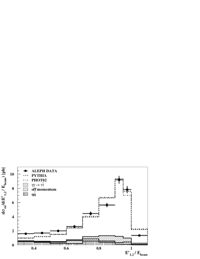
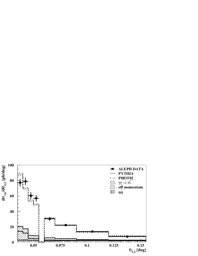
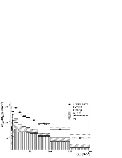
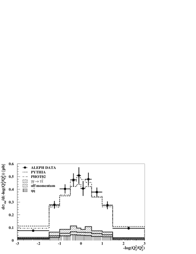
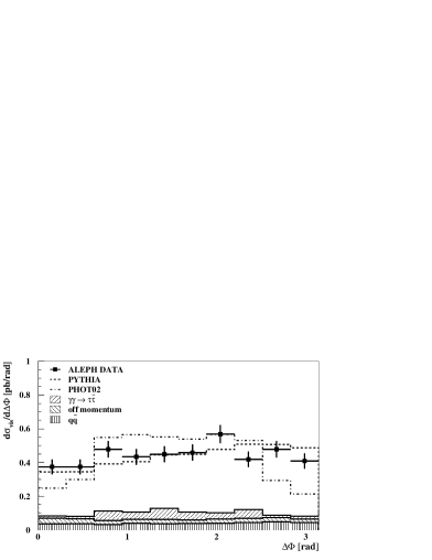
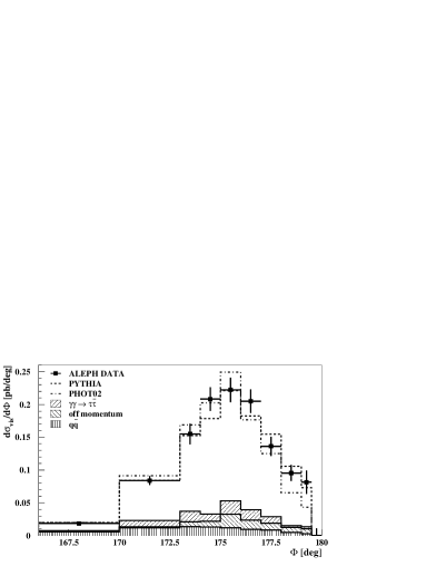
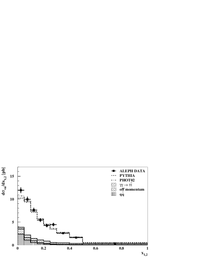
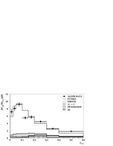
Figure 2: Differential cross sections as a function of various observables. Shown are (from top left to bottom right): The relative tag energy $E^{\prime}_{\mathrm{1,2}}/E_{\mathrm{beam}}$; the polar angle of the scattered electrons $\theta_{\mathrm{1,2}}$; the virtualities $Q^{2}_{i}$ of the photons; the ratio of the two virtualities, shown as $\Delta Q=-\log Q^{2}_{1}/Q^{2}_{2}$; the acoplanarity angle $\Delta\phi$ between the scattered electrons; the acolinearity $\Phi$ between the scattered electrons; the deep inelastic scattering variables $x_{i}$ and $y_{i}$. The plots contain the background contributions (filled areas), the PYTHIA and PHOT02 Monte Carlo predictions plus background (lines), and the data (points) with the statistical errors.

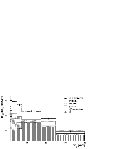
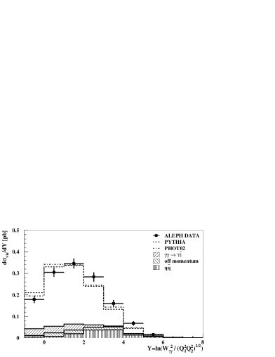
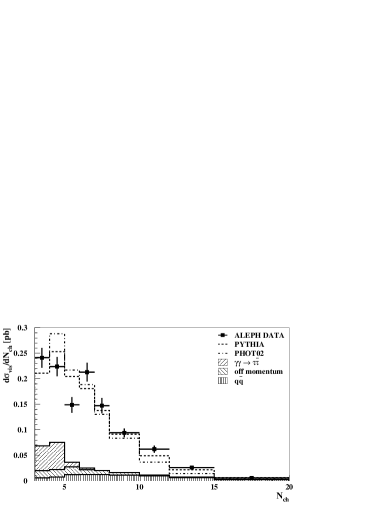
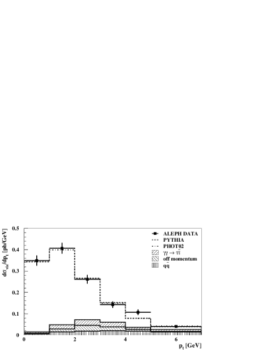
Figure 3: Differential cross sections as a function of various observables. Shown are (from top left to bottom right): The mass of the hadronic system $W_{\gamma\gamma}$; the quantity $Y=\log W_{\gamma\gamma}^{2}/\sqrt{Q^{2}_{1}Q^{2}_{2}}$; the number of charged tracks $N_{\mathrm{ch}}$; the pseudorapidity $\eta_{\mathrm{ch}}=-\log\tan(\theta_{\mathrm{ch}}/2)$ of the charged tracks; the number of neutral objects $N_{\mathrm{neutral}}$; the pseudorapidity $\eta_{\mathrm{neutral}}$ of the neutral objects; the relative total visible energy $E_{\mathrm{tot}}/2E_{\mathrm{beam}}$; the total transverse momentum $p_{\mathrm{t}}$ of the event with respect to the beam pipe. The plots contain the background contributions (filled areas), the PYTHIA and PHOT02 Monte Carlo predictions plus background (lines), and the data (points) with the statistical errors.

Several measured spectra are given in Figs. 2 and 3 showing the comparison between data and simulations after normalization.

5 Acceptance Corrections and Systematic Errors

A simple bin-by-bin method was applied to correct for detector inefficiencies. The correction factors were calculated for each bin as

$$\varepsilon_{\mathrm{bin}}=\frac{N_{\mathrm{true}}}{N_{\mathrm{detected}}}$$ (7)

where $N_{\mathrm{true}}$ is the number of generated events in a given bin and $N_{\mathrm{detected}}$ the number of detected events in the same bin according to the simulation. The corrected data values for a bin, $R_{\mathrm{cor}}$, were then derived from the measured values, $R_{\mathrm{visible}}$, by

$$R_{\mathrm{cor}}=(R_{\mathrm{visible}}-R_{\mathrm{background}})\varepsilon_{\mathrm{bin}}$$ (8)

where $R_{\mathrm{background}}$ is the expected background.

In order to estimate the systematic effect caused by an imperfect detector simulation all energy resolutions were varied by 10% (Fig. 3).

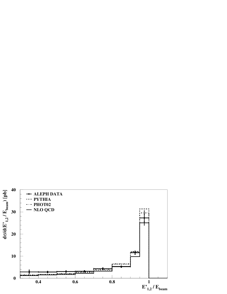
Figure 4: Differential cross section as a function of the energy of the scattered electrons $E_{\mathrm{1,2}}/E_{\mathrm{beam}}$

The uncertainty due to a possible shift in the energy scale of the luminosity monitors SICAL and LCAL (Fig. 4) was estimated by introducing an offset of 0.5 GeV to the measured energy. The polar and azimuthal angles of the electrons were shifted by 0.25 mrad and 0.5 mrad. These seemingly large adjustments were made to estimate a possible systematic uncertainty due to a poor description of small polar angles of the electrons (Fig. 5).

The cross sections of the background processes were changed conservatively by $\pm 10\%$.

The PHOT02 Monte Carlo simulation was used instead of PYTHIA to correct for detector effects. In both cases the systematic uncertainties due to statistical fluctuations in the Monte Carlo sample were small.

Systematic differences between the data collected in different years were not observed.

The systematic error was computed as the quadratic sum of the various contributions. The main contributions to the systematic error come from varying the energy resolutions and the tag energy.

6 Results

The measured cross sections, corrected for detector effects, are given in Figs. 4 to 13. The corresponding bin-contents are given in the Appendix. The results are compared with the PYTHIA and PHOT02 Monte Carlo models and the NLO QCD prediction [3].

Figure 4 shows the cross section as a function of the tag energy. The cross section predicted by the NLO QCD calculation comes out too low by $20\%$. The tail towards low energies is slightly underestimated by all models. The polar angle $\theta$ of the scattered electrons is given in Fig. 5. The first measured point (35 to 40 mrad) is overestimated by the Monte Carlo. The gap between SICAL and LCAL (55 to 60 mrad) is interpolated for the further results in Figs. 6 to 13.

The virtuality of the photons $Q^{2}_{i}$ are well simulated over the whole accessible range (Fig. 6). This also applies to the ratio of the two virtualities (Fig. 7).

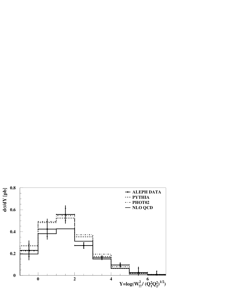
Figure 13: Differential cross section as a function of Y

The acoplanarity angle $\Delta\phi$ (Fig. 8) and the acolinearity $\Phi$ between the scattered electrons (Fig. 9) are well described by the PYTHIA prediction. The NLO QCD calculation yields a slightly too low cross section at large angles, and PHOT02 does not describe well the acoplanarity angle distribution. The mass of the hadronic system is again well reproduced by the Monte Carlo simulations. The NLO QCD calculation comes out with a slightly too low cross section for small masses (Fig. 10). The deep inelastic scattering variables $x_{i}$ (Fig. 11) and $y_{i}$ (Fig. 12) in data are well described by the Monte Carlo simulations. The NLO QCD calculation fails in reproducing the cross section as a function of $x_{i}$, while $y_{i}$ agress well. The cross section as a function of $Y$ is given in Fig. 13. Again the Monte Carlo simulations describe the measured spectrum well.

Finally the data are compared to BFKL predictions. The calculation was done for photons with virtualities of $12\,\mathrm{GeV}^{2}$ (90% of the data) and $38\,\mathrm{GeV}^{2}$ (10% of the data). Since this calculation assumes that both photons have the same virtuality, a further cut was added to the event selection [20]:

$$|\Delta Q|=|\log Q^{2}_{1}/Q^{2}_{2}|<1.0\ \ .$$ (9)

The whole analysis, including systematic error estimation, was redone with this new cut, which reduced the statistics by 40%.

The $\sigma_{\gamma\gamma}$ cross section [21, 22, 23] was extracted from the measured $\mathrm{e}^{+}\mathrm{e}^{-}$ cross section using GALUGA [24]. The resulting cross section as a function of $Y$ is plotted in Fig. 14, where it is compared to LO BFKL and NLO BFKL calculations [4, 5, 6, 7, 8]. In the LO BFKL calculation the Regge scale parameter was varied from $Q^{2}$ to $10Q^{2}$. Even at the lowest $Y$ values this calculation is barely in agreement with the data. The NLO BFKL calculation, however, with the Regge scale parameter varied from $Q^{2}$ to $4Q^{2}$ (solid curves) is consistent with the data.

7 Conclusions

The cross section for the process

$$\mathrm{e}^{+}\mathrm{e}^{-}\rightarrow\mathrm{e}^{+}\mathrm{e}^{-}\gamma\gamma\rightarrow\mathrm{e}^{+}\mathrm{e}^{-}\mathrm{hadrons}$$ (10)

has been measured using ALEPH data taken at $\mathrm{e}^{+}\mathrm{e}^{-}$ centre-of-mass energies $\sqrt{s}=188-209\,\mathrm{GeV}$ and corresponding to an integrated luminosity of $640\,\mathrm{pb}^{-1}$. The phase space is defined by the electron energies $E_{1,2}^{\prime}>0.3E_{\mathrm{beam}}$, the polar angles of the electrons $0.35\,\mathrm{mrad}<\theta_{1,2}<155\,\mathrm{mrad}$, and the mass of the hadronic system $W_{\gamma\gamma}>3\,\mathrm{GeV}/c^{2}$.

The differential cross section for $\mathrm{e}^{+}\mathrm{e}^{-}\rightarrow\mathrm{e}^{+}\mathrm{e}^{-}\gamma\gamma\rightarrow\mathrm{e}^{+}\mathrm{e}^{-}\mathrm{X}$, X being the hadronic final state, has been measured as a function of various event observables.

The majority of measured distributions are well described in shape by the PHOT02 and PYTHIA Monte Carlo models, but both required an adjustment to their normalization to match the data. The cross section of the PYTHIA Monte Carlo generator was reduced by 12% and the cross section extracted from PHOT02 was increased by 30%.

The NLO QCD prediction yields a slightly low cross section. With the exception of the deep inelastic scattering variable $x_{i}$ this calculation also gives a reasonable description of the data. Similar conclusions have been drawn by the L3 [25] and the OPAL [26] Collaborations.

A slight enhancement of the data with respect to the simulations is observed at high $Y$, but the steep rise of the cross section as predicted by LO BFKL is not observed in data. However, NLO BFKL is close in shape and normalization to the data.

Acknowledgements

We wish to thank our colleagues in the CERN accelerator divisions for the successful operation of LEP. We are indebted to the engineers and technicians in all our institutions for their contribution to the excellent performance of ALEPH. Those of us from non-member countries thank CERN for its hospitality.

Figure 5: Differential cross section as a function of the polar angle $\theta$ of the scattered electrons

Figure 6: Differential cross section as a function of the virtualities $Q^{2}_{1,2}$ of the two photons

Figure 7: Differential cross section as a function of the ratio of the two virtualities, shown as $\Delta Q=-\log Q^{2}_{1}/Q^{2}_{2}$

Figure 8: Differential cross section as a function of the acoplanarity angle $\Delta\phi$ between the scattered electrons.

Figure 9: Differential cross section as a function of the acolinearity $\Phi$ between the scattered electrons.

Figure 10: Differential cross section as a function of the mass of the hadronic system $W_{\gamma\gamma}$

Figure 11: Differential cross section as a function of the deep inelastic scattering variable $x_{i}$

Figure 12: Differential cross section as a function of the deep inelastic scattering variable $y_{i}$

Figure 14: The $\sigma_{\gamma\gamma}$ cross section as a function of $Y$ in comparison with LO BFKL and NLO BFKL, the range giving the uncertainty estimated from the variation of the Regge scale parameter from $Q^{2}$ to $10Q^{2}$ and from $Q^{2}$ to $4Q^{2}$, respectively.

Appendix

Table 2: Differential cross section as a function of the relative energy of the electrons $e_{\mathrm{1,2}}=\frac{E_{\mathrm{1,2}}^{\prime}}{E_{\mathrm{beam}}}$.

$e_{\mathrm{1,2}}$ bin		$d\sigma/de_{\mathrm{1,2}}\quad[\mathrm{pb}]$
		data			PYTHIA	PHOT02	QCD
0.30 –	0.40	2.85 $\pm$	0.47 $\pm$	1.03	1.37	1.51	1.18
0.40 –	0.50	2.78 $\pm$	0.39 $\pm$	0.30	1.69	1.74	1.50
0.50 –	0.60	3.01 $\pm$	0.37 $\pm$	0.32	1.98	2.14	1.69
0.60 –	0.70	3.12 $\pm$	0.36 $\pm$	0.10	2.63	2.78	2.18
0.70 –	0.80	4.36 $\pm$	0.36 $\pm$	0.21	3.72	3.94	3.20
0.80 –	0.90	5.19 $\pm$	0.36 $\pm$	0.27	6.35	6.51	5.31
0.90 –	0.95	11.51 $\pm$	0.78 $\pm$	0.40	11.86	12.06	9.76
0.95 –	1.00	27.24 $\pm$	1.75 $\pm$	2.99	31.33	29.54	25.02
		$\chi^{2}/$ NDF			23.3 / 7	20.2 / 7	34.6 / 8

Table 3: Differential cross section as a function of the polar angle $\theta$ of the scattered electrons.

$\theta$ bin		$d\sigma/d\theta\quad[\mathrm{pb/rad}]$
[rad]		data			PYTHIA	PHOT02	QCD
0.035 –	0.040	110.11 $\pm$	9.63 $\pm$	3.92	129.33	132.93	115.79
0.040 –	0.045	122.18 $\pm$	9.94 $\pm$	3.01	101.10	104.87	89.68
0.045 –	0.050	94.71 $\pm$	8.01 $\pm$	2.47	81.76	86.08	69.86
0.050 –	0.055	81.16 $\pm$	7.08 $\pm$	2.73	66.91	69.70	57.97
0.060 –	0.070	40.57 $\pm$	3.63 $\pm$	1.65	43.84	44.06	35.49
0.070 –	0.090	28.08 $\pm$	2.14 $\pm$	0.92	28.37	28.03	22.92
0.090 –	0.120	15.81 $\pm$	1.29 $\pm$	0.55	15.46	14.38	11.44
0.120 –	0.155	6.49 $\pm$	0.84 $\pm$	0.27	8.30	7.03	5.44
		$\chi^{2}/$ NDF			18.4 / 7	13.1 / 7	45.8 / 8

Table 4: Differential cross section as a function of the virtuality $Q^{2}_{1,2}$ of the photons.

$Q^{2}$ bin		$d\sigma/dQ^{2}_{i}\quad[\mathrm{pb/GeV^{2}}]$
[GeV]		data			PYTHIA	PHOT02	QCD
2.0 –	6.0	0.0133 $\pm$	0.0062 $\pm$	0.0056	0.0089	0.0131	0.0085
6.0 –	10.0	0.0852 $\pm$	0.0112 $\pm$	0.0059	0.0461	0.0638	0.0401
10.0 –	20.0	0.1290 $\pm$	0.0070 $\pm$	0.0052	0.1295	0.1462	0.1160
20.0 –	30.0	0.0785 $\pm$	0.0056 $\pm$	0.0161	0.0691	0.0682	0.0606
30.0 –	40.0	0.0415 $\pm$	0.0081 $\pm$	0.0073	0.0414	0.0393	0.0331
40.0 –	50.0	0.0263 $\pm$	0.0030 $\pm$	0.0013	0.0278	0.0256	0.0216
50.0 –	70.0	0.0160 $\pm$	0.0016 $\pm$	0.0004	0.0174	0.0165	0.0137
70.0 –	100.0	0.0111 $\pm$	0.0011 $\pm$	0.0008	0.0100	0.0084	0.0073
100.0 –	150.0	0.0038 $\pm$	0.0005 $\pm$	0.0003	0.0051	0.0038	0.0033
150.0 –	200.0	0.0010 $\pm$	0.0003 $\pm$	0.0002	0.0022	0.0013	0.0013
		$\chi^{2}/$ NDF			27.0 / 9	12.0 / 9	30.3 / 10

Table 5: Differential cross section as a function of the ratio of the virtualities of the two photons $\Delta Q=-\log\frac{Q_{1}^{2}}{Q_{2}^{2}}$.

$\Delta Q$ bin		$d\sigma/d\Delta Q\quad[\mathrm{pb}]$
[GeV]		data			PYTHIA	PHOT02	QCD
$-$3.0 –	$-$1.5	0.096 $\pm$	0.021 $\pm$	0.007	0.149	0.120	0.096
$-$1.5 –	$-$1.0	0.394 $\pm$	0.057 $\pm$	0.016	0.374	0.357	0.292
$-$1.0 –	$-$0.5	0.631 $\pm$	0.076 $\pm$	0.025	0.519	0.546	0.464
$-$0.5 –	$-$0.2	0.686 $\pm$	0.098 $\pm$	0.042	0.619	0.661	0.565
$-$0.2 –	0.0	0.749 $\pm$	0.122 $\pm$	0.034	0.623	0.755	0.611
0.0 –	0.2	0.664 $\pm$	0.127 $\pm$	0.044	0.638	0.763	0.633
0.2 –	0.5	0.736 $\pm$	0.105 $\pm$	0.043	0.612	0.709	0.566
0.5 –	1.0	0.620 $\pm$	0.083 $\pm$	0.035	0.524	0.538	0.451
1.0 –	1.5	0.403 $\pm$	0.062 $\pm$	0.023	0.383	0.354	0.276
1.5 –	3.0	0.122 $\pm$	0.021 $\pm$	0.005	0.147	0.120	0.095
		$\chi^{2}/$ NDF			13.1 / 9	4.7 / 9	20.9 / 10

Table 6: Differential cross section as a function of the acolinearity $\Phi$ of the scattered electron and the scattered positron.

$\Phi$ bin		$d\sigma/d\Phi\quad[\mathrm{pb/degree}]$
[degree]		data			PYTHIA	PHOT02	QCD
166.0 –	170.0	0.014 $\pm$	0.004 $\pm$	0.001	0.017	0.017	0.015
170.0 –	173.0	0.088 $\pm$	0.010 $\pm$	0.002	0.090	0.102	0.081
173.0 –	174.0	0.189 $\pm$	0.029 $\pm$	0.013	0.184	0.230	0.172
174.0 –	175.0	0.307 $\pm$	0.032 $\pm$	0.021	0.257	0.316	0.251
175.0 –	176.0	0.295 $\pm$	0.033 $\pm$	0.025	0.301	0.376	0.281
176.0 –	177.0	0.308 $\pm$	0.034 $\pm$	0.034	0.271	0.293	0.223
177.0 –	178.0	0.220 $\pm$	0.030 $\pm$	0.014	0.266	0.217	0.184
178.0 –	179.0	0.200 $\pm$	0.031 $\pm$	0.016	0.229	0.120	0.138
179.0 –	179.5	0.192 $\pm$	0.059 $\pm$	0.070	0.170	0.066	0.093
		$\chi^{2}/$ NDF			5.9 / 8	15.6 / 8	12.1 / 9

Table 7: Differential cross section as a function of the acoplanarity angle $\Delta\Phi$ of the scattered electron and the scattered positron.

$\Delta\phi$ bin		$d\sigma/d\Delta\phi\quad[\mathrm{pb/degree}]$
[degree]		data			PYTHIA	PHOT02	QCD
0.00 –	0.31	0.45 $\pm$	0.07 $\pm$	0.02	0.42	0.27	0.43
0.31 –	0.63	0.49 $\pm$	0.07 $\pm$	0.02	0.44	0.36	0.45
0.63 –	0.94	0.58 $\pm$	0.08 $\pm$	0.06	0.45	0.77	0.48
0.94 –	1.26	0.54 $\pm$	0.08 $\pm$	0.07	0.49	0.85	0.55
1.26 –	1.57	0.53 $\pm$	0.08 $\pm$	0.06	0.53	0.79	0.60
1.57 –	1.88	0.62 $\pm$	0.08 $\pm$	0.05	0.61	0.82	0.58
1.88 –	2.20	0.82 $\pm$	0.09 $\pm$	0.03	0.68	0.88	0.56
2.20 –	2.51	0.58 $\pm$	0.09 $\pm$	0.03	0.76	0.83	0.53
2.51 –	2.83	0.83 $\pm$	0.10 $\pm$	0.08	0.89	0.41	0.50
2.83 –	$\pi$	0.88 $\pm$	0.13 $\pm$	0.14	0.99	0.29	0.48
		$\chi^{2}/$ NDF			8.7 / 9	60.7 / 9	19.5 / 10

Table 8: Differential cross section as a function of the mass $W_{\gamma\gamma}$ of the hadronic system.

$W_{\gamma\gamma}$ bin		$d\sigma/dW_{\gamma\gamma}\quad[\mathrm{pb/GeV}]$
[GeV]		data			PYTHIA	PHOT02	QCD
3.0 –	5.0	0.1409 $\pm$	0.0164 $\pm$	0.0257	0.1499	0.1307	0.0996
5.0 –	10.0	0.1263 $\pm$	0.0095 $\pm$	0.0033	0.1334	0.1380	0.1019
10.0 –	15.0	0.0763 $\pm$	0.0072 $\pm$	0.0032	0.0787	0.0814	0.0665
15.0 –	35.0	0.0276 $\pm$	0.0023 $\pm$	0.0023	0.0246	0.0244	0.0205
35.0 –	50.0	0.0102 $\pm$	0.0020 $\pm$	0.0021	0.0050	0.0052	0.0043
50.0 –	80.0	0.0005	${}^{+0.0010}_{-0.0005}$ $\pm$	0.0020	0.0012	0.0013	0.0011
		$\chi^{2}/$ NDF			5.3 / 5	6.4 / 5	18.0 / 6

Table 9: Differential cross section as a function of the Björken variable $x_{1,2}$.

$x_{i}$ bin		$d\sigma/dx_{i}\quad[\mathrm{pb}]$
		data			PYTHIA	PHOT02	QCD
0.00 –	0.05	17.71 $\pm$	1.38 $\pm$	2.00	14.11	15.88	12.17
0.05 –	0.10	14.48 $\pm$	1.05 $\pm$	1.13	13.51	13.70	10.84
0.10 –	0.15	11.97 $\pm$	0.95 $\pm$	0.77	11.12	11.00	8.99
0.15 –	0.20	8.20 $\pm$	0.79 $\pm$	0.44	8.67	8.62	7.02
0.20 –	0.25	6.62 $\pm$	0.72 $\pm$	0.56	7.03	6.98	5.61
0.25 –	0.30	7.31 $\pm$	0.70 $\pm$	0.43	5.40	5.50	4.66
0.30 –	0.40	3.71 $\pm$	0.36 $\pm$	0.22	3.68	3.96	3.45
0.40 –	0.50	2.19 $\pm$	0.28 $\pm$	0.14	2.25	2.31	2.07
0.50 –	1.00	0.42 $\pm$	0.06 $\pm$	0.09	0.70	0.46	0.46
		$\chi^{2}/$ NDF			16.0 / 8	7.3 / 8	30.6 / 9

Table 10: Differential cross section as a function of the Björken variable $y_{1,2}$.

$y$ bin		$d\sigma/dy_{i}\quad[\mathrm{pb}]$
		data			PYTHIA	PHOT02	QCD
0.000 –	0.025	51.28 $\pm$	5.54 $\pm$	7.34	40.37	37.49	31.79
0.025 –	0.050	19.41 $\pm$	1.99 $\pm$	2.07	21.48	20.73	17.61
0.050 –	0.100	11.68 $\pm$	0.79 $\pm$	0.49	12.02	12.27	9.93
0.100 –	0.150	5.16 $\pm$	0.50 $\pm$	0.35	7.54	7.55	6.19
0.150 –	0.200	5.39 $\pm$	0.52 $\pm$	0.21	5.31	5.61	4.49
0.200 –	0.300	4.43 $\pm$	0.36 $\pm$	0.22	3.74	3.94	3.21
0.300 –	0.400	3.15 $\pm$	0.36 $\pm$	0.09	2.64	2.79	2.20
0.400 –	0.600	2.85 $\pm$	0.27 $\pm$	0.26	1.84	1.95	1.60
0.600 –	0.800	1.41 $\pm$	0.23 $\pm$	0.50	0.69	0.76	0.59
		$\chi^{2}/$ NDF			31.1 / 8	28.1 / 8	42.4 / 9

Table 11: Differential cross section as a function of $Y$.

$Y$ bin		$d\sigma/dY\quad[\mathrm{pb}]$
		data			PYTHIA	PHOT02	QCD
$-$1.0 –	0.0	0.224 $\pm$	0.028 $\pm$	0.031	0.270	0.223	0.195
0.0 –	1.0	0.437 $\pm$	0.039 $\pm$	0.015	0.483	0.493	0.381
1.0 –	2.0	0.542 $\pm$	0.045 $\pm$	0.022	0.523	0.545	0.425
2.0 –	3.0	0.422 $\pm$	0.040 $\pm$	0.030	0.352	0.370	0.312
3.0 –	4.0	0.227 $\pm$	0.035 $\pm$	0.017	0.171	0.194	0.149
4.0 –	5.0	0.117 $\pm$	0.026 $\pm$	0.024	0.062	0.079	0.065
5.0 –	6.0	0.026	${}^{+0.040}_{-0.020}$ $\pm$	0.013	0.019	0.025	0.012
6.0 –	7.0	0.008	${}^{+0.030}_{-0.008}$ $\pm$	0.005	0.004	0.009	0.004
		$\chi^{2}/$ NDF			9.3 / 7	5.2 / 7	19.3 / 8

References

- [1] T. Sjöstrand et al., High-energy-physics event generation with PYTHIA 6.1, Comput. Phys. Commun. 135 (2001) 238.
- [2] ALEPH Collaboration, An experimental study of hadrons at LEP, Phys. Lett. B313 (1993) 509.
- [3] M. Cacciari, V. Del Duca, S. Frixione and Z. Trocsanyi, QCD radiative corrections to hadrons, JHEP 02 (2001) 29.
- [4] E.A. Kuraev, L.N. Lipatov and V.S. Fadin, The Pomeranchuk singularity in nonabelian gauge theories, Sov. Phys. JETP 45 (1977) 199.
- [5] I.I. Balitsky and L.N. Lipatov, The Pomeranchuk singularity in quantum chromodynamics, Sov. J. Nucl. Phys. 28 (1978) 822.
- [6] V.T. Kim, L.N. Lipatov and G.B. Pivovarov, The next-to-leading dynamics of the BFKL pomeron, Proceedings of the 29th International Symposium on Multiparticle Dynamics: QCD and Multiparticle Production - ISMD ’99, Providence, RI, USA, Eds.: I. Sarcevic and C.-I. Tan, World Sci., Singapore (2000) 79.
- [7] V.T. Kim, L.N. Lipatov and G.B. Pivovarov, The next-to-leading BFKL pomeron with optimal renormalization, Proceedings of the International Conference on Elastic and Diffractive Scattering 1999, Protvino, Russia, Eds.: V.A. Petrov and A.V. Prokudin, World Sci., Singapore (2000) 237.
- [8] V.T. Kim, private communication.
- [9] C. Friberg and T. Sjöstrand, Total cross sections and event properties from real to virtual photons, JHEP 09 (2000) 010.
- [10] C. Friberg and T. Sjöstrand, Effects of longitudinal photons, Phys. Lett. B492 (2000) 123.
- [11] R. Engel and J. Ranft, Hadronic photon-photon interactions at high energies, Phys. Rev. D54 (1996) 4244.
- [12] J.A.M. Vermaseren, Two photon processes at very high energies, Nucl. Phys. B229 (1983) 347.
- [13] G. Cochard and P. Kessler (eds.), Gamma gamma collisions, proceedings, international workshop, Amiens, France, April 8-12, 1980, Lecture Notes In Physics 134, (Berlin: Springer 1980).
- [14] R. Bhattacharya, J. Smith and G. Grammer, Jr. Two photon production processes at high energy, Phys. Rev. D15 (1977) 3267.
- [15] I.F. Ginzburg and V.G. Serbo, Some comments on the total hadron cross-section at high energy, Phys. Lett. B109 (1982) 231.
- [16] G. Bonneau, M.G. Gourdin and F. Martin, Inelastic lepton anti-lepton scattering and the two photon exchange approximation, Nucl. Phys. B54 (1973) 573.
- [17] S. Jadach, B.F.L. Ward and Z. Was, The Monte Carlo program KORALZ, version 4.0, for lepton or quark pair production at LEP / SLC energies, Comput. Phys. Commun. 79 (1994) 503.
- [18] G. Marchesini et al., HERWIG: A Monte Carlo event generator for simulating hadron emission reactions with interfering gluons, Comput. Phys. Commun. 67 (1992) 465.
-
[19]
ALEPH Collaboration,
ALEPH: A detector for electron-positron annihilations at LEP,
Nucl. Instrum. and Meth. A294 (1990) 121;
ALEPH Collaboration,
Performance of the ALEPH detector at LEP,
Nucl. Instrum. and Meth. A360 (1995) 481;
B. Mours et al., The design, construction and performance of the ALEPH silicon vertex detector, Nucl. Instrum. and Meth. A379 (1996) 101. - [20] C. Ewerz, private communication.
- [21] V.M. Budnev, I.F. Ginzburg, G.V. Meledin and V.G. Serbo, The two photon particle production mechanism, physical problems, applications, equivalent photon approximation, Phys. Rept. 15 (1974) 181.
- [22] R. Nisius, The photon structure from deep inelastic electron photon scattering, Phys. Rept. 332 (2000) 165.
- [23] S.J. Brodsky, F. Hautmann and D.E. Soper, Virtual photon scattering at high energies as a probe of the short distance pomeron, Phys. Rev. D56 (1997) 6957.
- [24] G.A. Schuler, Two-photon physics with GALUGA 2.0, Comput. Phys. Commun. 108 (1998) 279.
- [25] L3 Collaboration, Measurement of the cross-section for the process hadrons at LEP, Phys. Lett. B453 (1999) 333.
- [26] OPAL Collaboration, Measurement of the hadronic cross-section for the scattering of two virtual photons at LEP, Eur. Phys. J. C24 (2002) 17.