Experimental measurement of muon $(g-2)$

The muon $(g-2)$ experiment at Brookhaven National Laboratory has measured the anomalous magnetic moment of the positive muon with a precision of 0.7 ppm. This paper presents that result, concentrating on some of the important experimental issues that arise in extracting the anomalous precession frequency from the data.

1 Concept

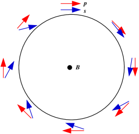
Figure 1: (a) Motion of the muon spin vector relative to its momentum vector. (b) Trajectories followed by several decay positrons of varying energies.

The spin of the muon generates a magnetic moment whose strength is described by a dimensionless quantity $g_{\mu}$, the gyromagnetic ratio:

$$\vec{\mu}=g_{\mu}\left(\frac{e}{2m}\right)\vec{s}~{}.$$

The Brookhaven National Laboratory AGS E821 muon $(g-2)$ experiment measures the anomalous part $a_{\mu}$ of the gyromagnetic ratio, defined by $a_{\mu}=\frac{1}{2}(g_{\mu}-2)$. For a pointlike Dirac particle, $a_{\mu}=0$. It acquires a nonzero value only through radiative corrections. It may be measured experimentally with great precision; the published data from E821 have a precision of 0.7 parts per million (ppm). It may also be calculated precisely in the context of the standard model, taking into account contributions from the electromagnetic and weak interactions, which are understood well, and from hadronic processes, which are more troublesome. The current state of these calculations is described in this volume by A. Nyffeler and A. Höcker. The nominal precision of these results is also at the level of 0.7 ppm, but inconsistent values are obtained depending on the hadron production cross section data that constitute an essential input. Once this situation is resolved, it will be possible to draw conclusions from a comparison of the experimental and theoretical results. Such a comparison may either yield evidence for or a constraint against physics beyond the standard model.

The idealized muon $(g-2)$ experiment places a polarized ensemble of muons in a uniform magnetic field at $t=0$. They follow circular orbits in this field with a cyclotron frequency of

$$\vec{\omega}_{c}=\frac{e\vec{B}}{m\gamma}~{}.$$

Meanwhile, the field rotates their spin at a frequency of

$$\vec{\omega}_{s}=g_{\mu}\frac{e}{2m}\vec{B}+(\gamma-1)\frac{e\vec{B}}{m\gamma}~{}.$$

This frequency includes a term resulting from the Thomas precession $\!{}^{{\bf?}}$ because the muon is in a rotating reference frame. The difference between the cyclotron and spin precession frequencies is the so-called anomalous precession frequency:

$$\vec{\omega}_{a}=\vec{\omega}_{s}-\vec{\omega}_{c}=\frac{e}{m}a_{\mu}\vec{B}~{}.$$ (1)

This frequency is the rate at which the spin turns with respect to the momentum, and it is therefore the apparent precession frequency from the point of view of an observer in the laboratory, as shown in Figure 1. It is proportional to $a_{\mu}$, not to $g_{\mu}$, so $a_{\mu}$ may in principle be determined directly by measuring $\omega_{a}$ and $B$ and performing a little arithmetic. In practice, though, the magnetic field is mapped using NMR magnetometers,$\!{}^{{\bf?}}$ which measure the spin precession frequency $\omega_{p}$ of protons at rest in the field. To minimize the number of external constants required, Equation 1 is rewritten as

$$a_{\mu} = \frac{\frac{\omega_{a}}{\omega_{p}}}{\frac{\omega_{s}}{\omega_{p}}-\frac{\omega_{a}}{\omega_{p}}}=\frac{R_{\omega}}{\lambda-R_{\omega}}~{}{\rm with}$$

$$R_{\omega} = \frac{\omega_{a}}{\omega_{p}}~{}{\rm and}~{}\lambda=\frac{\omega_{s}}{\omega_{p}}=\frac{\mu_{\mu}}{\mu_{p}}=3.183\,345\,39(10)~{}.$$

This value of $\lambda$ is determined from experiments on the hyperfine structure of muonium conducted at Los Alamos National Laboratory, together with some theoretical input.$\!{}^{{\bf?},{\bf?}}$

Eventually, essentially all of the muons decay via the three-body process $\mu^{+}\rightarrow~{}e^{+}\nu_{e}\bar{\nu}_{\mu}$. Because the resulting positrons have a lower energy than that of the muon, they curl in toward a detector as shown in Figure 1. In the CM frame, the kinematic distribution of the decay positrons is peaked along the direction of the spin of the parent muon: $\!{}^{{\bf?}}$

$$\frac{dP}{dy~{}d\Omega}=n(y)[1+A(y)\cos\theta_{s}]~{}{\rm where}$$

$$n(y)=y^{2}(3-2y)~{}{\rm and}~{}A(y)=\frac{2y-1}{3-2y}~{}.$$

In these expressions, $y=2E/(m_{\mu}-m_{e})$ is the normalized energy of the positron and $\theta_{s}$ is the CM angle between the muon’s spin and the positron’s momentum. As the spin turns with a frequency $\omega_{a}$, this “searchlight” of decay positrons moves with it. Approximating both the muon and positron as fully relativistic particles so that $E=p$, the boost into the laboratory frame is described by

$$E_{lab}=\gamma E_{CM}(1+\cos\theta_{CM})~{},$$

where $\theta_{CM}$ is the CM angle between the positron momentum and the forward direction defined by the muon momentum. To have a high energy in the laboratory, a decay positron must therefore both have a high energy in the CM frame and also be directed forward. Consequently, the boost translates the angular sweep of the CM frame into a modulation of the energy distribution in the laboratory frame. By counting the number of decay positrons exceeding a laboratory energy threshold as a function of time after injection, one obtains a spectrum that is described by the functional form

$$N(t)=Ne^{-t/\tau}[1-A\cos(\omega_{a}t+\phi_{a})]~{}.$$ (2)

The frequency $\omega_{a}$ may then be determined by fitting this functional form to the observed spectrum.

The real-world experiment is quite similar to this simple outline. The magnetic field is provided by a C-shaped superferric storage ring magnet $\!{}^{{\bf?}}$. Its 1.45 T field is uniform at the level of 1 ppm over the storage region after averaging over the azimuthal coordinate. The muon beam enters the ring through a field-free region produced by a superconducting inflector magnet.$\!{}^{{\bf?}}$ From this point, a circular trajectory would simply lead it around for a single turn where it would be lost on the inflector housing. Therefore, it is necessary to kick it onto the central orbit with a pulsed magnet.$\!{}^{{\bf?}}$ To avoid perturbing the field during the measuring period, the kicker contains no iron, and its pulse is only a little longer than one cyclotron period.

In the radial dimension, the uniform dipole field has a focusing effect: all circular orbits are closed regardless of the initial radial position and angle, provided only that they do not strike an obstruction. In the vertical dimension, however, additional focusing is required: a particle with even a rather small initial vertical angle will quickly spiral up or down without bound out of the storage volume. Consequently, electric quadrupoles $\!{}^{{\bf?}}$ are placed inside the storage ring vacuum chambers. They are plates on which a static electrical charge is placed during the measuring period, leading to a linear restoring force for particles that are off-center vertically. The electric field appears as an additional magnetic field in the muon’s rest frame, so Equation 1 is modified: $\!{}^{{\bf?},{\bf?}}$

$$\vec{\omega}_{a}=\vec{\omega}_{s}-\vec{\omega}_{c}=\frac{e}{m}\left[a_{\mu}\vec{B}-\left(a_{\mu}-\frac{1}{\gamma^{2}-1}\right)(\vec{\beta}\times\vec{E})\right]~{}.$$

However, the term proportional to $(\vec{\beta}\times\vec{E})$ is eliminated by choosing a “magic” $\gamma\approx 29.3$, corresponding to a muon momentum of $3.09~{}{\rm GeV}/c$. Consequently, it is not necessary to have precise knowledge of the quadrupole field.

2 Determination of energies and times

Decay positrons are detected by lead/scintillating fiber electromagnetic calorimeters $\!{}^{{\bf?}}$ located inside the storage ring. The signals from these calorimeters are recorded by waveform digitizers, which sample the photomultiplier output at 400 MHz. The resulting waveforms are similar to traces on a digital oscilloscope. They are processed into energies and arrival times by the analysis software.

A potential systematic bias arises from overlapping pulses in the calorimeters. The $(g-2)$ phase $\phi_{a}$ in Equation 2 is determined primarily by the time of flight from the decay vertex to the detector. Consequently, it varies with positron energy by about 20 mrad from 1.4 to 3.2 GeV. Overlapping pulses appear to have a high energy, but they carry the phase of their lower-energy constituents. The concentration of overlapping pulses varies from early to late times after injection because their number is proportional to the square of the instantaneous muon decay rate. They cause the average phase to shift as a function of time, thereby pulling the measured frequency.

The first line of defense against overlapping pulses is separation. The algorithm used to determine times and energies from the waveforms is capable of resolving pulses that arrive as little as 3.5 ns apart. The procedure is based on the principle that the recorded samples look like an averaged pulse shape, translated in time and scaled with energy. First, an average pulse shape is constructed for each detector. Then, an optimization procedure is applied to each digitized interval, varying the assumed time, amplitude, and pedestal to minimize the least-squares difference

$$\sum_{i\,\in\,{\rm samples}}[S_{i}-P-\sum_{j\,\in\,{\rm pulses}}A_{j}f_{i}(t_{j})]^{2}$$

between the recorded samples $S_{i}$ and the average pulse shape $f(t)$. When the fit to a single pulse is insufficient, the model is extended to include additional pulses.

Nevertheless, some residual overlapping pulses inevitably remain. They are subtracted by forming out-of-time coincidences. Each pulse defines a time region of approximately 40 ns which is guaranteed to have been digitized by the WFD. Additional pulses found in these regions are artificially combined to simulate the distribution of true overlapping pulses. These constructed distributions may then be subtracted from the data or, equivalently, incorporated into the fitting function.

3 Betatron motion

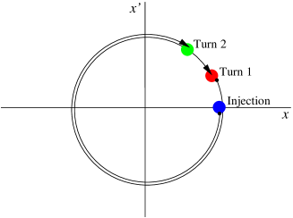
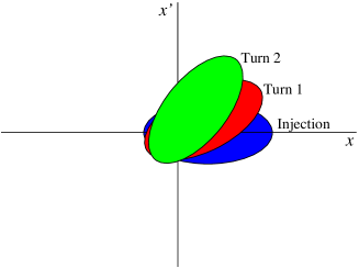
Figure 2: The radial betatron motion of (a) a single particle, and (b) a distribution of particles, illustrating why the CBO appear at the beat frequency $\omega_{c}-\omega_{x}$. The centroid and width of the projections of the distribution onto the $x$ and $x^{\prime}$ axes clearly move with each turn as well.

The confining electric quadrupole field, together with the main dipole field, leads to simple harmonic motion of each particle in both the radial and vertical dimensions. It is described by

$$x(t) = x_{e}+A_{x}\cos(\omega_{x}t+\phi_{x})$$

$$y(t) = A_{y}\cos(\omega_{y}t+\phi_{y})$$

where

$$\omega_{x}=\omega_{c}\sqrt{1-n}~{},\omega_{y}=\omega_{c}\sqrt{n}~{}{\rm and}~{}$$

$$n=\frac{\partial E_{r}}{\partial r}\frac{R_{0}}{\beta B_{0}}\approx 0.137$$

If the accepted phase space of the storage ring were uniformly populated, then the betatron motion would not be relevant. Although the individual particles would oscillate, the $(x,x^{\prime})$ and $(y,y^{\prime})$ distributions as a whole would not. However, for practical reasons, the inflector is not matched to the storage ring, so only a subset of the phase space is filled. As viewed by an observer standing at a single azimuthal position inside the storage ring, the radial phase space distribution appears to rotate at the beat frequency $\omega_{CBO}=\omega_{c}-\omega_{x}$. The beam centroid oscillates radially toward and away from the detector. While the beam moves toward a detector on one side of the ring, it moves away from the detector on the opposite side. Thus, CBO effects vary smoothly through $2\pi$ around the storage ring. There is also a small effect from oscillations of the width of the distribution. These phenomena are illustrated in Figure 2.

The CBO are visible in the recorded time spectrum primarily because the detector acceptance is a function of the decay vertex radius as well as azimuthal position and positron energy. This acceptance function is established by two competing mechanisms. Geometrically, particles that come from a smaller radius are more likely to hit the detector than those from large radii because their momentum has a larger azimuthal component. However, they also pass through obstacles such as the quadrupole or kicker plates at a more glancing angle, increasing the probability that they will begin their electromagnetic shower there, outside the detector. The balance between these two mechanisms shifts as a function of positron energy. The fact that the acceptance is a function of radial position leads to an overall modulation of the time spectrum at the frequency $\omega_{CBO}$, at the level of 1 percent. Meanwhile, the fact that the function is energy-dependent leads to a modulation of the asymmetry $A$ in Equation 2. Finally, the rotation of the angular ($x^{\prime}$) distribution modulates the phase $\phi_{a}$, because the average spin direction turns along with the average momentum. These additional modulations may be added to the fitting function of Equation 2, which now looks substantially more complicated:

$$f(t) = e^{-t/\tau}N\{[1+C_{1}(t)]-A[1+C_{1}(t)+C_{2}(t)]\cos(\omega_{a}t+\phi_{a}+C_{3}(t))\}$$

$$C_{1,2,3}(t) = E(t)A_{c1,2,3}\cos(\omega_{CBO}t+\phi_{c1,2,3})$$

$E(t)$ is an empirically-determined function that accounts for the the coherence time of the CBO. The factor $C_{1}(t)$ describes the overall modulation of the count rate, while $C_{2}(t)$ and $C_{3}(t)$ deal with the more subtle effects on $A$ and $\phi_{a}$.

The systematic bias caused by these distortions of the time spectrum is enhanced by an unfortunate coincidence of frequencies. For the quadrupole voltages used in the 1999 and 2000 running periods, $\omega_{CBO}\approx 465~{}{\rm kHz}$ is nearly $2\omega_{a}$. Consequently, to the extent that the CBO introduce a background in the time spectrum at the difference frequency $\omega_{CBO}-\omega_{a}$, they perturb the fitted value of $\omega_{a}$. Figure 3 shows the results of fits to the spectrum of each detector to a function that includes only the primary effect $C_{1}(t)$ of the CBO, with $C_{2}(t)=C_{3}(t)=0$. The fitted value of $\omega_{a}$ is not consistent across detectors, but rather varies continuously by about $\pm 4$ ppm around the ring. This behavior is explained by Figure 3, which shows the Fourier transform of the difference between the time spectrum for the detectors on one half of the ring and the functional form to which it was fit. A distinct peak at the sideband frequency $\omega_{CBO}-\omega_{a}$ is quite visible when the spectrum is fit by the ideal function of Equation 2, and it is not eliminated by including only $C_{1}(t)$. With the full treatment including all three CBO effects, this peak vanishes into the noise. As the CBO bias is eliminated by fitting for these effects, the apparent dependence of the value of $\omega_{a}$ on ring position also vanishes.

4 Determination of $\omega_{a}$

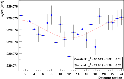
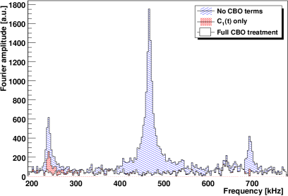
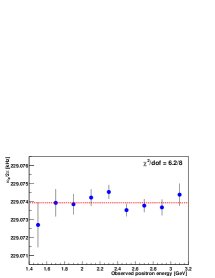
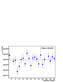
Figure 3: (a) Fitted value of $\omega_{a}$ as a function of detector station number with a simplified function where $C_{2}(t)=C_{3}(t)=0$. (b) Fourier transform of the residuals following fits to the spectra of detector stations 13-24. (c) The fitted value of $\omega_{a}$ by energy bin and (d) by station, indicating consistency in both cases.

Four independent extractions of $\omega_{a}$ were performed, based on two independent implementations of the pulse fitting procedure. The analyses were done “blind,” without precise knowledge of the magnetic field. Two of these analyses were conventional, setting a single energy threshold. One analysis formed a asymmetry signal by dividing the data into four subsets and combining them in a ratio that cancels out the exponential baseline. The fourth analysis divided the data into narrow energy bins, fit them separately, and combined the results. Some of the analyses included the CBO modulations $C_{2}(t)$ and $C_{3}(t)$ in the fitting function, while others chose to rely on the reduction of the bias from the CBO by an order of magnitude in the average of the detectors. In the end, the results of the four analyses agreed with each other within statistical and systematic expectations. The results of the energy-binned analysis, which included all CBO-related terms, are shown in Figure 3. They demonstrate that the fitted value of $\omega_{a}$ is consistent in this case as a function of energy and detector number. The four independent analyses were averaged to give

$$\omega_{a}/2\pi=229\,074.11(0.14)(0.07)~{}{\rm Hz}$$

This value has been corrected by 0.76 $\pm$ 0.03 ppm to account for the effects of vertical oscillations and electric fields. The significant contributions to the systematic uncertainty are, in addition to overlapping pulses and CBO, muon losses and detector gain variations during the measuring period. The magnitudes of the contributions from different sources varied to some extent among the four analyses, but all agreed on a total of 0.3 ppm.

5 Magnetic field measurement

The magnetic field is mapped using NMR magnetometers,$\!{}^{{\bf?}}$ which measure the spin precession frequency $\omega_{p}$ of protons at rest in the field. A set of 17 of these devices is mounted on a trolley that is driven around the inside of the storage region every few days during the running period, yielding a multipole map as a function of azimuth. Between trolley runs, changes in the field are tracked by fixed NMR probes located just outside the vacuum chambers. The trolley probes were calibrated against a standard spherical water probe whose absolute calibration is known at the level of 0.05 ppm.$\!{}^{{\bf?}}$ Over a period of several years, the field in the storage ring was iteratively shimmed for improved uniformity. Because the variation over the storage aperture is at the level 1 ppm, it is not necessary to know the distribution of muons very well.

Two independent analyses of the $\omega_{p}$ data were conducted; again, they were blind, performed without knowledge of $\omega_{a}$. The analyses were in agreement and found the result

$$\omega_{p}/2\pi=61\,791\,595(15)~{}{\rm Hz}$$

The largest contributions to the total error of 0.24 ppm are from the calibration of the trolley probes against the standard, non-linearity in the trolley position determination, and the reproducibility of the relationship between the field values measured by the trolley and the fixed probes.

6 Results and conclusions

The “world average” value of $a_{\mu}$, which is dominated by the data set collected in 2000, is $\!{}^{{\bf?}}$

$$a_{\mu}^{exp;avg}=11\,659\,203(8)\times 10^{-10}~{}.$$

Davier and collaborators provide two standard model theory results; they differ in the experimental input used to the hadronic contributions. They are $\!{}^{{\bf?}}$

$$a_{\mu}^{th;ee} = 11\,659\,169.3(7.8)\times 10^{-10}~{}{\rm and}~{}a_{\mu}^{th;\tau}=11\,659\,193.6(6.8)\times 10^{-10}~{}.$$

The first result gives a discrepancy of 3.0 standard deviations, while the second indicates agreement at the level of 0.9 standard deviations.

At the moment, it does not seem appropriate to draw conclusions from the comparison of theory and experiment for $a_{\mu}$; the theory value is still in flux. The CMD-2 collaboration continues to check its hadron production cross section results, and alternative approaches such as radiative return $\!{}^{{\bf?}}$ and lattice calculations $\!{}^{{\bf?}}$ may hold some promise. Also, Martin and Wells have demonstrated that it is possible to make some theoretical progress even with the current ambiguity. They show $\!{}^{{\bf?}}$ that a significant part of the parameter space of the minimal supersymmetric standard model (MSSM) is excluded at the level of five standard deviations, even after assigning a very generous uncertainty to the hadronic effects.

References

References

- [1] L. Thomas, Phil. Mag. 3, 1 (1927).
- [2] R. Prigl et al., Nucl. Instrum. Meth. A374, 118 (1996).
- [3] W. Liu et al., Phys. Rev. Lett. 82, 711 (1999).
- [4] M. Nio and T. Kinoshita, Phys. Rev. D55, 7267 (1997), [hep-ph/9702218].
- [5] F. Farley and E. Picasso, The muon -2 experiments, in Quantum Electrodynamics, edited by T. Kinoshita, pp. 479–559, World Scientific, Singapore, 1990.
- [6] G. T. Danby et al., Nucl. Instrum. Meth. A457, 151 (2001).
- [7] A. Yamamoto et al., Nucl. Instrum. Meth. A491, 23 (2002).
- [8] E. Efstathiadis et al., Nucl. Instrum. Meth. A496, 8 (2003).
- [9] Y. K. Semertzidis et al., Nucl. Instrum. Meth. A, accepted for publication.
- [10] V. Bargmann, L. Michel and V. Telegdi, Phys. Rev. Lett. 2, 453 (1959).
- [11] J. Jackson, Classical Electrodynamics, 3rd ed. (John Wiley and Sons, New York, 1999).
- [12] S. A. Sedykh et al., Nucl. Instrum. Meth. A455, 346 (2000).
- [13] X. Fei, V. Hughes and R. Prigl, Nucl. Instrum. Meth. A394, 349 (1997).
- [14] Muon -2 Collaboration, G. W. Bennett et al., Phys. Rev. Lett. 89, 101804 (2002), [hep-ex/0208001].
- [15] M. Davier, S. Eidelman, A. Höcker and Z. Zhang, Eur. Phys. J. C27, 497 (2003), [hep-ph/0208177].
- [16] KLOE Collaboration, G. Venanzoni et al., hep-ex/0210013.
- [17] T. Blum, hep-lat/0212018.
- [18] S. P. Martin and J. D. Wells, Phys. Rev. D67, 015002 (2003), [hep-ph/0209309].