Collider Experiment:
Strings, Branes and Extra Dimensions

Abstract

Selected topics showcasing the exploration for new physics using colliders; presented at TASI 2001.

Contents

toc

1 Preface

The subject of the Theoretical Advanced Study Institute summer 2001 school was “STRINGS, BRANES and EXTRA DIMENSIONS”. Although not too many years ago a course on collider physics would had been an unorthodox inclusion to the curriculum of a such titled school, today there are attempts to connect strings, branes and extra dimensions with experiment. Indeed string phenomenology is not an oxymoron, to the delight of all. I was particularly content to see young theorists spending time calculating the beam power in a future linear electron accelerator and the dollar sum necessary to pay the electric bill in a year. I was also very impressed that there were students who already knew what a trigger is and why we use it.

It took at least a generation of inspired physicists and also math experts to move from field theories to string theory, and a concurrent of technowizzes and inquiring minds to discover and measure with exquisite precision the theory describing nature at the most fundamental length scales yet explored: the Standard Model. Although it seemed briefly that theory and experiment are fast growing apart we witness today a remarkable exchange between the two, and a tendency to almost believe that by putting separate small bricks of knowledge together, one day preferably soon, the complete edifice of nature will be exactly blueprinted and raised.

The lectures were organized in three sections. The first one is devoted to accelerators. There is no doubt that these machines gave birth to the field we call High Energy Physics and filled in turn the Particles and Fields data-books. And there is no substitute for these machines. They are evolving, with the purpose of exploring the physics at the highest energy reachable or equivalently the physics at the shortest length scale. The second is an overview of the kind of experiments that lead us from atoms all the way down to quarks and a brief summary of the particle physics jargon used when we report results. And the third is analysis examples and interpretation of results when looking for new physics. Since the school’s interests is on string theory I will give a supersymmetry search example and an example of the search for extra dimensions with collider data.

2 Accelerators

There are at least 10,000 accelerators in the world, most of them put to action in solving every day problems. A world-wide search by W.H. Scharf and O.A. Chomicki [1] reports 112 accelerators of more than 1 GeV. A third of these are used in high energy physics research. The rest are mostly synchrotron light sources. About 5000 accelerating machines of lower energy are used in medicine (radiotherapy, biomedical research and isotope production). About as many are used in industry, usually for ion implantation and surface physics. The latest sterilization via irradiation made the news in the post September 11 time when all the letters to Washington were collected to be irradiated for fear of anthrax. A great review of accelerators for medical applications has been written by Ugo Amaldi [2].

We are familiar with the use of high energy lepton and hadron accelerators for particle physics. Present investigations are focused on the search for the Higgs boson, neutrino oscillations, heavy quark physics, the production of supersymmetric particles and even the geometry and geography of spacetime. There is little doubt that this type of research is connected intimately with cosmology in re-creating particles and interactions from the first instant of the Big Bang through the era when nuclei were formed by the more fundamental particles. The data accumulated from high energy particle collisions are essential in formulating and stimulating cosmological models and in helping understand the origin of the dark matter and perhaps even the dark energy in the universe.

I would like at this point to remark that it seems to me that when the director of the Office of Science and Technology Policy, Dr. Marburger, wrote  [3] that at “ some point we will have to stop building accelerators” he meant it in a similar way that NASA will stop building space shuttles. This is to say that new technologies will necessarily be employed in endeavors of tremendous magnitude such as the exploration of the universe in all scales; the exploration itself will not cease.

Accelerators	Number in use
(1) High-energy more than 1GeV	112
(2) Radiotherapy	$>$4000
(3) Research/Biomedical Research	$\sim$800 $\sim$5000
(4) Medical radioisotope production	$\sim$ 200
(5) Industry	$\sim$1500
(6) Ion implanters	$>$2000
(7) Surface modification centers and research	$\sim$1000
(8) Synchrotron radiation sources	50
total (in 1995) $\sim$10000

Table 1: Statistics of operating accelerators (1995).

2.1 DC Accelerators

In the beginning of the century there was chemistry, philosophy (cosmic ray research was being published in journals of philosophy), and by 1932 we had nuclear physics when the neutron was discovered by Chadwick. Three more particles were known by then; the electron (J.J. Thompson in 1897 passed electrons through crossed E and B fields, measured the velocity and then e/m of the electron), the proton (Rutherford, 1913 - he called the proton the hydrogen atom nucleus) and the photon (Max Planck, black body radiation in quanta of $h\nu$, Einstein photoelectric effect, Compton X-ray scattering from electrons as if particles. The photon was actually named by a chemist.)

During the first part of the century natural radioactivity and cosmic rays were the source of energetic particles for atomic physics research. In 1906 Rutherford bombarded a mica sheet with alpha particles from a natural radioactive source (Rutherford scattering). Natural sources are limited in energy and intensity. In 1928 Cockroft and Walton started thinking about building an accelerator to use at the Cavendish Laboratory. In 1932 the apparatus was finished and used to split lithium nuclei with 400 keV protons. The measurement of the binding energy in this experiment provided the first experimental verification of Einstein’s mass-energy relationship (known since 1905). This was the start of particle accelerators for nuclear research. The very first ones were direct voltage accelerators like the Cockroft and Walton (rectifier generator up to 1 MV), the Van de Graff generator (up to 10 MV in high-pressure tank containing dry nitrogen or freon to avoid sparking) and the tandem electrostatic accelerator (the accelerator is known as tandem because the ions, at the beginning negative, undergo a double acceleration: they are attracted by the positive central electrode, pass in a cleaner who makes them positive, and they are then pushed back by the electrode; up to maybe 35 MV, Vivitron Strasbourg, in operation now at 20 MV).

2.2 AC Accelerators

Ising in 1924 proposed the first particle accelerator that would give the particles more energy than the maximum voltage in the system. He proposed an electron linear accelerator with drift tubes (but did not build it). In 1928 Wideroe used an alternating 25 kV voltage with 1 MHz frequency applied over two gaps and produced 50 keV potassium ions. The Wideroe type linac comprises a series of conducting drift tubes. Alternate drift tubes are connected to the same terminal of the RF generator. The frequency is such that when a particle goes through the gap it sees the accelerating field and when the field becomes decelerating the particle is shielded inside the drift tube. As the particle gains in energy and velocity the structure periods must be longer in order to be in sync. At very high frequencies (so that the structure does not become inconveniently long) the open drift-tube scheme needs to be enclosed to form a cavity or series of cavities.

If one applies Ising’s resonant principle in a homogeneous magnetic field the particle would be bent back to the same RF gap twice for each period. This is Lawrence’s and Livingston’s fixed-frequency cyclotron (the initial was less than one foot in diameter and could accelerate protons to 1.25 MeV). The resonance condition in the cyclotron is obtained by choosing the RF period equal to the cyclotron period, which is independent of the particle velocity and the orbit radius ; it depends on the $q/m$ ratio and the magnetic field. Particles that pass the gap near the peak of the RF voltage would continue to do so every half turn moving in ever increasing half-circles (spiraling) until they reach the edge of the magnetic field or until they become relativistic and slip back with respect to the gap voltage. The intrinsic limit was confronted in the late thirties at about 25 MeV for protons and 50 MeV for deuterons and alpha particles. The cyclotron consisted of two “D” shaped regions in vacuum, called dees with a gap separating them and a magnetic field applied perpendicular to the dees. As the proton beam crosses the gap it experiences an electric field which gives the proton a kick and increases its energy. It gets an energy increase every time it crosses the gap. The frequency of the applied electric field is constant, while the radius of the proton beam keeps increasing.

Synchro-cyclotron -or the frequency-modulated cyclotron- was the remedy for the relativistic limit in which the revolution frequency decreases with increasing energy, and the frequency of the accelerating voltage must also be correspondingly decreased. Although this is necessary, it in not sufficient to maintain sync, because the natural energy spread in a bunch of relativistic ions causes a spread in their cyclotron frequencies, and thus longitudinal focusing is required to maintain the “bunch”. The problem was overcome by McMillan and Veksler who discovered the principle of phase stability in 1944. The effect of phase stability is that a bunch of charged particles with an energy spread can be kept bunched throughout the acceleration cycle by injecting them at a suitable phase of the RF cycle. Synchro-cyclotrons can be used to accelerate protons up to 1 GeV. The higher energy is obtained at the expense of intensity (number of particles in the bunch) since the pulsed beam has less intensity compared to a continuous beam. To achieve transverse stability of the beam the field should be decreasing with radius according to an inverse power law. At Berkeley they found (the hard way) that the magnetic field has to decrease slightly with increasing orbit radius to prevent the particles from getting lost.

For electrons the cyclotron is useless as they are very quickly relativistic. The solution was the betatron, a device that has found applications in laboratories and hospitals. It was conceived again by Wideroe; Kernst built the first betatron in 1941 and Kernst and Serber published a paper on “betatron oscillations” the same year. In 1950 Kernst built the world’s largest betatron. In a betatron, the electromagnet is powered with an AC current at 50 to 200 Hz. The magnetic field guides the particles in a circular orbit, but because it is a changing magnetic field, it induces a circumferential voltage which accelerates the particles. The guide field was carefully shaped and given a radial gradient in order to provide vertical and horizontal beam stability. If the electron path is to remain at constant radius the magnetic field must increase as the electron energy increases. The increasing field results in increasing magnetic flux through the orbits which then induces the force that increases the energy of the electrons. The magnetic flux through the orbit must be twice the bending field in order to keep the beam at the same radius.

The betatron was soon replaced by the synchrotron which is an accelerator that combines the properties of the cyclotron and those of the betatron. McMillan and Veksler already discusses the idea of synchronous acceleration in their cyclotron papers. The first synchrotron (Cosmotron) was a 3 GeV proton accelerator built in 1952 at Brookhaven National Laboratory (BNL). The machine had straight sections and a guide field similar to the betatron with a bending field to keep the particles on a circular orbit and appropriate radial gradient to achieve vertical and horizontal stability. Acceleration was achieved by RF voltage at the revolution frequency. As the particle energy increases the field is also increased at a rate that keeps the particles in approximately the same orbit at all energies. This means that the RF voltage frequency should be increasing (compare with cyclotron). Many large synchrotron machines followed the Cosmotron. The Tevatron at Fermilab is one of them, accelerating protons and antiprotons to approximately 1000 GeV.

In all accelerators build before 1952 the transverse stability of the beam depended on what is now called weak focusing in the magnet system. The guide field decreases slightly with increasing radius in the vicinity of the particle orbit and this gradient is the same all around the circumference of the magnet. The tolerance on the gradient is severe and sets limits to such an accelerator (believed to be around 10 GeV in the early fifties). The aperture needed to contain the beam becomes very large and the magnet becomes very bulky and costly. The invention of the alternating-gradient principle by Christofilos and independently by Courant, Livingston and Snyder in 1952 changed this picture. As a matter of fact, machines in the range of 10-100 TeV seem already technically possible. The limitation is the cost. Alternating-gradient or “strong” focusing is directly analogous to a result in geometrical optics, that the combined focal length of two appropriately spaced lenses of equal strength will be overall focusing when one lens is focusing and the other defocusing. Such a system remains focusing for quite some range of the focal length values of the two lenses. A quadrupole lense focuses on one plane and defocuses on the orthogonal plane. An appropriate arrangement of quadrupoles can be altogether focusing in both planes. Structures based on this principle are called alternating gradient (AG) structures.

Although the circular machines took over for some time, the linear machines were revived after WW II with advances in ultra-high frequency technologies. At Berkeley a proton linac was built by Alvarez (1946) who employed the war-developed radar technology and enclosed the entire drift tube structure in a resonant cavity to reduce losses. Since then this type of accelerator has been widely used as an injector (with injection energies reaching 200 MeV) for large proton and heavy-ion synchrotrons (e.g. the Fermilab linac and the HERA linac at Deutches Electronen Synchrotron (DESY) in Hamburg, Germany). The largest proton linear accelerator today is the the 800 MeV proton linac at the Los Alamos Neutron Science Center (LANSE). The largest electron linear accelerator in operation is the 50 GeV linac at the Stanford Linear Accelerator Center (SLAC). Linear accelerators, like betatrons previously, have become very popular in fields outside particle physics (e.g materials science, biomedical research, and medicine).

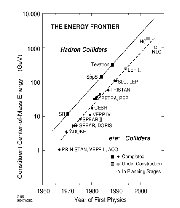
Figure 1: The effective constituent energy of existing and planned colliders and the year of first physics results from each (after [4]).

An increase in beam energy of about 1.5 orders of magnitude per decade is illustrated by the Livingston chart shown in Figure  1. While the energy increases by 8 orders of magnitude the cost per GeV of a typical accelerator has been drastically reduced. But what is most amazing is that while each type of acceleration is coming to saturation relatively fast, there is an advance in technology that allows a different idea on acceleration to kick in. Examples: the invention of the alternating gradient focusing in the fifties, the colliding beams in the sixties, superconducting magnet technology and stochastic cooling in the seventies and eighties.

2.3 Colliders/Storage Rings

In high energy physics experiments, the type and number of particles brought into collision and their center of mass energy characterize an interaction. The center of mass energy $E_{CM}$ made available when a synchrotron beam of energy $E_{b}$ hits a fixed target is approximately

$$\sqrt{s}=E_{CM}=(2m_{target}E_{b})^{1/2}$$ (1)

The center of mass energy when colliding head-on two beams of energy $E_{b}^{\prime}$ is

$$\sqrt{s}=E_{CM}=2E_{b}^{\prime}$$ (2)

The purpose of storage rings is to make head-on collisions possible with a useful interaction rate. At the Tevatron the maximum proton energy is about 1000 GeV. In the $p\bar{p}$ collider mode the center of mass energy is $\sqrt{s}=E_{CM}=2000$ GeV. In the fixed target mode it is $\sqrt{s}=E_{CM}=41$ GeV.

The fixed target collisions produce a variety of secondary particles from the target that can be collected and focused into secondary beams. Also in fixed target collisions the achieved luminosities are extremely high. The reaction rate $R$ is $R=L~{}\times~{}\sigma$, where $L$ is the luminosity and $\sigma$ is the cross section. This implies that $L=(N_{beam}/\rm{sec})(N_{target}/\rm cm^{2})$. Luminosity is measured usually in cm^-2sec^-1. A fixed target experiment can have luminosity as high as $10^{37}$ cm^-2sec^-1. In a high luminosity collider experiment the luminosity is of the order of $10^{32}$ cm^-2sec^-1.

What is the limitation on the energy for an accelerator storage ring? For proton accelerators it is the maximum magnetic field to bend the particles ($R_{ring}(m)=P(GeV)/0.3B(Tesla)$). For electron storage rings it is the energy lost to synchrotron radiation per revolution, $U\approx 0.0885E(GeV)^{4}R(m)^{-1}$. (For relativistic proton beams this is $\approx 7.79^{-15}E(\rm{GeV})^{4}R(\rm{m})^{-1}$). The largest electron-positron storage ring was the 27 km LEP ring at CERN in Geneva. It started running at a beam energy of about 50 GeV: this meant that 200 MeV per turn should be supplied by the RF to make up for the synchrotron radiation loss. When it ran at 100 GeV, a factor of two higher in energy, the energy loss per turn was 3.2 GeV, a factor of 16 increase in losses! A linear electron-positron accelerator (such as the SLC, the Stanford Linear Collider) avoids the problem of synchrotron radiation. It is expected that all future electron-positron machines at higher energy than LEP will be linear.

Note that a monoenergetic proton (antiproton) beam is equivalent to a wide-band parton beam (where parton$\equiv$quarks, antiquarks, gluons), described by momentum distribution $dn_{i}/dp$ (structure function, $i$ specifies the parton type, i.e. $u,d,g,\bar{u},\bar{d}...$). Proton structure functions are measured in deep inelastic scattering experiments.

Some of the advantages of hadron collisions include the simultaneous study of a wide energy interval, therefore there is no requirement for precise tuning of the machine energy; the greater variety of initial state quantum numbers e.g. $u+\bar{d}\rightarrow W^{+},~{}\bar{u}+d\rightarrow W^{-}$; the fact that the maximum energy is much higher than the maximum energy of $e^{+}e^{-}$ machines; and finally that hadron collisions are the only way to study parton-parton collisions (including gluon-gluon). Some of the disadvantages are the huge cross sections for uninteresting events; the multiple parton collisions in the same hadron collision that result in complicated final states; and that the center-of-mass frame of the colliding partons is not at rest at the lab frame.

Table 2 lists some present, historic and proposed colliders.

Proton Fixed Target Accelerators
Name	Lab	Location	GeV	status
PS	CERN	Geneva	28	inactive
AGS	BNL	Long Island	32	active
SPS	CERN	Geneva	450	active
Tevatron	FNAL	Chicago	1000	active
Electron Fixed Target Accelerators
LINAC	SLAC	Stanford	50	active
Proton Colliding Beam Machines
ISR	CERN	Geneva	31$p\times$ 31$p$	inactive
S$p\bar{p}$S	CERN	Geneva	310$p\times$ 310$\bar{p}$	inactive
Tevatron	FNAL	Chicago	1000$p\times$ 1000$\bar{p}$	active
SSC	SSCL	Dallas	20000$p\times$ 20000$\bar{p}$	canceled
LHC	CERN	Geneva	7000$p\times$ 7000$p$	2007
Electron Colliding Beam Machines
SPEAR	SLAC	Stanford	4$e^{-}\times~{}4e^{+}$	inactive
DORIS	DESY	Hamburg	5$e^{-}\times~{}5e^{+}$	inactive
BES	BES	Beijing	4$e^{-}\times~{}4e^{+}$	active
CESR	Cornell	Ithaca	8$e^{-}\times~{}8e^{+}$	active
PEP	SLAC	Stanford	15$e^{-}\times~{}15e^{+}$	inactive
PEPII	SLAC	Stanford	9$e^{-}\times~{}3e^{+}$	active
PETRA	DESY	Hamburg	23$e^{-}\times~{}23e^{+}$	inactive
TRISTAN	KEK	Tokyo	30$e^{-}\times~{}30e^{+}$	inactive
KEK B	KEKB	Tokyo	8$e^{-}\times~{}3.5e^{+}$	active
SLC	SLAC	Stanford	50$e^{-}\times~{}50e^{+}$	active
LEPII	CERN	Geneva	200$e^{-}\times~{}200e^{+}$	inactive
Electron-Proton colliding Beam Machines
HERA	DESY	Hamburg	30$e^{-}\times~{}820p$	active
Future Electron-Positron Collider Study Collaborations
JLC	-	KEKB	(stage I) 125$e^{-}\times~{}125e^{+}$	R&D
NLC	-	SLAC	400$e^{-}\times~{}400e^{+}$	R&D
TESLA	-	DESY	400$e^{-}\times~{}400e^{+}$	R&D
CLIC	-	CERN	1500$e^{-}\times~{}1500e^{+}$	R&D
Future Hadron Collider Study Collaborations
VLHC	FNAL	Chicago	40000$p\times$ 40000$p$	R&D

Table 2: Present, historic(including cancelled) and proposed colliders

2.4 Future Colliders

We saw that the highest energy circular electron machine has been LEP. In order to go any higher in energy in electron-positron collisions, we need to build the collider on a straight line. The luminosity in terms of the configuration of the beams is $L=\frac{f_{coll}N^{2}}{S}$ where $f_{coll}$ is the number of bunch collisions per second, $N$ is the number of particles in a bunch and $S$ is the beam cross-sectional area at the collision point. In a linear collider clearly $f_{coll}$ is much smaller than in a circular collider. The number of particles $N$ in a bunch is similar or smaller. Therefore to achieve worthwhile luminosities it is imperative that the beam emittance $S$ be much smaller. A linear collider needs very high accelerating gradient to keep the site length reasonable and very high power efficiency to keep the cost under control. As we noted the beams need to be generated with extremely small emittance which has to be preserved during acceleration. At the collision point the beams have to be tightly focused. Small emittances can be achieved by preparing the beam through what is called a damping ring and making use of the synchrotron radiation. The acceleration is achieved by microwave cavities which can be superconducting or normal conducting, and the frequency choice is based on the achievable accelerating gradient. There are at least two different designs under development: The NLC/JLC design that uses normal conducting copper cavities at low frequency (11.424 GHz or X-band) which is also referred to as warm design, and the TESLA design that uses supeconducting niobium cavities, a technology that is power consumption effective (there is extremely small power dissipation in the cavity walls) but thought to be very expensive until recently. This is referred to as cold design because the cavities need to be kept at very low temperatures. Linear collider accelerating structures can also be used to drive free electron lasers, with important applications for chemistry, materials science, plasma research and life sciences research.

A post-LHC and probably post-LC collider that accelerates and collides electron and positron beams with center of mass 3-5 TeV is envisioned in the CLIC design. It is based on the two-beam acceleration method in which the RF power for sections of the main linac is extracted from a secondary, low-energy, high-intensity electron beam running parallel to the main linac.

The next hadron collider proposed is the VLHC . A design study group has developed the basic parameters, technology/construction challenges and cost of a proton-proton collider with center of mass energy greater than 30 TeV, that would allow the eventual operation of a collider with center of mass energy greater than 150 TeV in the same tunnel. The machine would involve two phases, one with low-field magnets and one with high-field magnets for the energy upgrade in the same 233 km ring.

It is not included in the table, but extensive study and research is geared towards the feasibility and potential of high energy high luminosity muon colliders operating at a center-of-mass energy in the range 100 GeV - 4 TeV. The high intensity muon source needed for muon colliders can also be used to feed a muon storage ring neutrino source (neutrino factory). The enthusiasm in recent years for a muon collider is due to ionization cooling that allows for very bright muon beams.

One lesson from the Livingston plot is that a new technology can push the collision energy and drive high energy research. Indeed accelerator technology is also moving towards alternative directions. High-gradient plasma wakefield acceleration is one. The plasma-wave acceleration process is dramatically strong and may lead to very high energy beams with reasonable size accelerators.

3 From atoms to quarks, Rutherford redux

The kind of experiments we perform to probe the structure of matter belong to three categories: scattering, spectroscopy and break-up experiments. The results of such experiments brought us from the atom to the nucleus, to hadrons, to quarks.

Geiger and Marsden reported in 1906 the measurements of how $\alpha$ particles (the nuclei of He atoms) were deflected by thin metal foils. They wrote “it seems surprising that some of the $\alpha$ particles, as the experiment shows, can be turned within a layer of 6$\times 10^{-5}$ cm of gold through an angle of 90^∘, and even more”. Rutherford later said he was amazed as if he had seen a bullet bounce back from hitting a sheet of paper. It took two years to find the explanation. The atom was known to be neutral and to be containing negatively charged electrons of mass very much less than the mass of the atom. So how was the positively charged mass distributed within the atom? Thompson had concluded that the scattering of the $\alpha$ particles was a result of “a multitude of small scatterings by the atoms of the matter traversed”. This was called the soft model. However “a simple calculation based on probability shows that the chance of an $\alpha$ particle being deflected through 90^∘ is vanishingly small”. Rutherford continued “It seems reasonable to assume that the deflection through a large angle is due to a single atomic encounter, for the chance of a second encounter of the type to produce a large deflection must be in most cases exceedingly small. A simple calculation shows that the atom must be a seat of an intense electric field in order to produce such a large deflection in a single encounter”. According to the soft model the distribution of scattered particles should fall off exponentially with the angle of deflection; the departure of the experimental distribution from this exponential form is the signal for hard scattering. The soft model was wrong. Geiger and Marsden found that 1 in 20,000 $\alpha$ particles was turned at 90^∘ or more in passing through a thin foil of gold; The calculation of the soft model predicted one in 10³⁵⁰⁰. The nuclear atom was born with a hard constituent , the small massive positively charged nucleus. Rutherford calculated the angular distribution expected from his nuclear model and he obtained the famous $\sin^{4}(\phi/2)$ law, where $\phi$ is the scattering angle.

At almost the same time Bohr (1913) proposed the model for the dynamics of the nuclear atom, based on a blend of classical mechanics and the early quantum theory. This gave an excellent account of the spectroscopy of the hydrogen. Beginning with the experiments of Frank and Hertz the evidence for quantized energy levels was confirmed in the inelastic scattering of electrons from atoms.

The gross features of atomic structure were described well by the nonrelativistic quantum mechanics of point-like electrons interacting with each other and with a point-like nucleus, via Coulomb forces.

As accelerator technology developed it became possible to get beams of much higher energy. From the de Broglie $\lambda=h/p$ relationship it is clear that the resolving power of the beam becomes much finer and deviations from the Rutherford formula for charged particles scattering (which assumed point-like $\alpha$’s and point-like nucleus) could be observed. And they did! At SLAC in 1950 an electron beam of 126 MeV (instead of $\alpha$’s) was used on a target of gold and the angular distribution of the electrons scattered elastically fell below the point-nucleus prediction. (qualitatively this is due to wave mechanical diffraction effects over a finite volume on the nucleus). The observed distribution is a product of two factors: the scattering from a single point-like target (a la Rutherford with quantum mechanical corrections, spin, recoil etc.) and a “form factor” which is characteristic of the spatial extension of the target’s charge density.

From the charge density distribution it became clear that the nucleus has a charge radius of about 1-2 fm (1 fm=$10^{-15}$ m); In heavier nuclei of mass number $A$ the radius goes as $A^{1/3}$ fm. If the nucleus has a finite spatial extension, it is not point-like. As with atoms, inelastic electron scattering from nuclei reveals that the nucleus can be excited into a sequence of quantized energy states (confirmed by spectroscopy).

Nuclei therefore must contain constituents distributed over a size of a few fermis, whose internal quantized motion lead to the observed nuclear spectra involving energy differences of order a few MeV.

Chadwick discovered the neutron in 1932 establishing to a good approximation that nuclei are neutrons and protons (generically called nucleons). Since the neutron was neutral, a new force with range of nuclear dimensions was necessary to bind the nucleons in the nuclei. And it must be very much stronger than the electromagnetic force since it has to counterbalance the “uncertainty” energy ($\approx$20 MeV; the repulsive electromagnetic potential energy between two protons at 1 fm distance is ten times smaller, well below the nucleon rest energy).

Why all this? The typical scale of size and energy are quite different for atoms and nuclei. The excitation energies in atoms are in general insufficiently large to excite the nucleus: hence the nucleus appears as a small inert point-like core. Only when excited by appropriately higher energy beams it reveals that it has a structure. Or in other words the nuclear degrees of freedom are frozen at the atomic scale.

To figure out whether the nucleons are point-like the picture we already developed is repeated once again. First elastic scattering results of electrons from nucleons (Hofstadter) revealed that the proton has a well defined form factor, indicating approximately exponential distribution of charge with an $rms$ radius of about 0.8 fermi. Also the magnetic moments of the nucleons have a similar exponential spatial distribution. Inelastic scattering results, as expected, showed signs of nucleon spectroscopy which could be interpreted as internal motions of constituents. For example in the scattering of energetic electrons from protons there is one large elastic peak (at the energy of the electron beam) and other peaks that correspond to excitations of the recoiling system. The interpretation of the data is a hairy story: several excited recoil states contribute to the same peak and even the apparently featureless regions conceal structure. In one of the first experiments that used close to 5 GeV electrons, only the first of the two peaks beyond the elastic had a somewhat simple interpretation: It corresponded exactly to a long established resonant state observed in pion-nucleon scattering and denoted by $\Delta$. Four charge combinations correspond to the accessible pion-nucleon channels: $\pi^{+}p,~{}\pi^{+}n(\pi^{0}p),~{}\pi^{-}p~{}(\pi^{0}n),~{}\pi^{-}n$. The results of such “baryon spectroscopy” experiments revealed an elaborate and parallel scheme as the atomic and nuclear previously. One series of levels comes in two charged combinations (charged and neutral) and is built on the proton and neutron as ground states; the other comes in four charge combinations (–,0,+,++) with the $\Delta$s as ground state.

Yukawa predicted the pion as the quantum of the short-range nuclear forces. In the 60s the pion turned out to be the ground state of excited states forming charge triplets. Lets note again that we are looking at the excitations of the constituents of composite systems. Gell-Mann and Zweig proposed that the nucleon-like states (baryons), are made of three 1/2 spin constituents: the quarks. The mesons are quark-antiquark bound states. Baryons and mesons are called collectively hadrons. As in the nuclear case the simple interpretation of the hadronic charge multiplets is that the states are built out of two types of constituents differing by one unit is charge - hence its constituents appeared fractionally charged. the assignment was that the two constituents were the up (u) and down (d) with 2/3 and -1/3 charge. The series of proton would then be $uud$ and the neutron $udd$ while the $\Delta^{++}$ would be $uuu$. The forces between the quarks must be charge independent to have this kind of excited states. Lets point here that the typical energy level differences in nuclei are measured in MeV. For the majority of nuclear phenomena the neutrons and protons remain in their ground unexcited states and the hadronic excitations are being typically of order MeV; the quark-ian, hadronic degrees of freedom are largely frozen in nuclear physics. People did not like the quarks; They really thought it was nonsense. Nevertheless a very simple “shell model” approach of the nucleon was able to give an excellent description of the hadronic spectra in terms of three quarks states and bound states of quark-antiquark. So now, how would we try to see those quarks directly? We need to think Rutherford scattering again and extend the inelastic electron scattering measurements to larger angles. The elastic peak will fall off rapidly due to the exponential fall off of the form factor. The same is true for the other distinct peaks; this indicates that the excited nucleon states have some finite spatial extension. The bizarre thing is that for large energy transfer the curve does not fall as the angle increases. In other words for large enough energy transfer the electrons bounce backwards just as the $\alpha$s did in the Geiger-Marsden experiment. This suggests hard constituents! This basic idea was applied in 1968 in so-called deep inelastic scattering experiments by Friedman, Kendall and Taylor in which very energetic electrons were scattered off of protons. The energy was sufficient to probe distances shorter than the radius of the proton, and it was discovered that all the mass and charge of the proton was concentrated in smaller components, spin 1/2 hadronic constituents called “partons” which were later identified with quarks. A lot of spectroscopy and scattering data became available in the ’70s and still people used the quarks as mathematical elements that help systematize a bunch of complicated data. In fact the following quote is attributed to Gell-Mann: “A search for stable quarks of charge -1/3 or +2/3 and/or stable di-quarks of charge -2/3 or +1/3 at the highest energy accelerators would help reassure us of the non-existence of real quarks”. Indeed quarks have not been seen as single isolated particles. When you smash hadrons at high energies, where you expect a quark what you observe downstream is a lot more hadrons - not fractionally charged quarks. The explanation of this quarky behavior – that they don’t exist as single isolated particles but only as groups “confined” to hadronic volumes – lies in the nature of the interquark force. November 1974 was a revolution of quarks: A new series of mesonic (quark-antiquark) spectra, the $J/\psi$ particles, were discovered, with quantum number characteristics of fermion-antifermion states. The $J/\psi$ spectrum is very well described in terms of $c\bar{c}$ states where $c$ is a new quark: the charm. The $c\bar{c}$ is called charmonium after the $e^{+}e^{-}$ positronium. There is a funny resemblance between the energy states of the charmonium with those of the positronium given that the positronium is bound via electromagnetic forces while the charmonium via strong forces.

Back to Rutherford again. We saw how the large angle large energy transfer electron scattering from nucleons provided evidence for “hard constituents”. What if we collide two nucleons? With a “soft” model of the nucleons we expect some sort of an exponential fall off of the observed “reaction products” as a function of their angle to the beam direction. On a “hard” model we should see prominent “events” at wide angles, corresponding to collisions between the constituents. The hard scattered quarks are converted into two roughly collimated ’jets’ of hadrons. These jets and their angular distributions provide indirect evidence of quarks. At $p\bar{p}$ collisions at CERN jets were observed in the 80s when CERN achieved with SPS the largest momentum transfers. Clear evidence of hadronic jets associated with primary quark processes were observed earlier in electron-positron collisions.

If quarks are not point-like we expect to see at higher energies, where the sub-quarkian degrees of freedom unfreeze perhaps at the Tevatron and the LHC, deviations from the theory similar to the deviations observed in the deep inelastic scattering experiments.

3.1 Technical handbook

The fragments of a high energy collision in matters of nanoseconds have decayed and/or left the detectors. In the early times of particle experiments an event was a picture in a bubble chamber for example, of the trail the particles left when ionizing a medium. Now an event is an electronic collection of the trails many particles left in a multiple complex of detectors. We are taking a little detour here to define some jargon particle physicists use, to discuss briefly what is the modern process of particle detection and what is the data analysis after all. To start, there is a physics collision for which we have a theoretical model to describe the particle interaction (we draw a Feynman graph). The fragments of the collision decay and interact with the detector material (we have for example multiple scattering). The detector is responding (there is noise, cross-talk, resolution, response function, alignment, temperature, efficiency…) and the real-time data selection (trigger) together with the data acquisition system give out the raw data (in the form of bytes; we read out addresses, ADC and TDC values and bit patterns). The analysis consists of converting the raw data to physics quantities. We apply the detector response (e.g. calibration, alignment) and from the interaction with the detector material we perform pattern recognition and identification. From this we reconstruct the particles’ decays and get results based on the characterization of the physics collision. We compare the results with the expectations by means of a reverse path that simulates the physics process calculated theoretically and driven through a computational model of the detector, the trigger and data acquisition path (Monte Carlo). The challenge is to select the useful data and record them with minimum loss (deadtime) when the detector and accelerator is running properly; and of course to analyze them and acquire results that are statistically rather than systematically limited. When the statistical uncertainty becomes smaller than the systematic uncertainty, it is time to build a new experiment for this measurement.

To give an example, in a hadronic collision at CMS in 2007, the interaction rate is 40 MHz (corresponding to data volume of 1000 TB/sec). The first level of data selection is hardware implemented and by using specific low level analysis reduces the data to 75 kHz rate (corresponding to data volume of 75 GB/sec). The second level of judging whether an event is going to be further retained is implemented with embedded processors that reduce the data rate to 5 Hz (5 GB/sec). The third level of the trigger is a farm of commodity CPUs that records data at 100 Hz (100 MB/sec). These data are being recorded for offline analysis. The final data volume depends on the physics selection trigger and for example we expect at the first phase of the Tevatron Run II to have between 1 and 8 petabytes per experiment. The improvement in high energy experiments is multifold. Better accelerator design and controls give higher energies and collision rates. Better trigger architecture is making best use of the detector subsystems. Better storage, networks and analysis algorithms contribute to precise and statistically significant results. Large CPU and clever algorithms improve the simulations and theoretical calculations that in turn enable the discovery of new physics in the data.

To summarize the jargon: trigger is a fast, rigid and primitive, usually hardware implemented selection applied on raw data or even analog signals from the detectors. Triggers have levels that an event passes through or fails. The trigger system and algorithms are emulated so that the signals are driven through a computational model of the trigger path, and the results are compared with the acquired data for diagnostic purposes. The efficiency of a multilevel trigger path is measured in datasets coming from orthogonal trigger paths (e.g. you want to measure the efficiency of a multilevel missing energy trigger in a dataset of events that come from a trigger that has no missing energy in its requirements). The duration of time when the data acquisition system cannot accept new data (usually because it is busy with current data) is called deadtime. To go faster modern experiments are running parallel data acquisition on sub-detector systems that are ending in fanned out triggers (data streams); the combination of the fragments of data from the detector subsystems is the event building. A filter is a later selection after the trigger, which is usually software implemented and can be sophisticated. Reconstruction is the coding that converts the sparsified hardware bytes to physics objects (tracks, vertices, tags etc.) A computer farm is a dedicated set of processors and associated networks used to run filters, event reconstruction, simulation etc. Efficiency is the probability to pass an event (signal or background). Enhancement is the enrichment of the data sample after a selection is applied.

4 Bottom-top experimental approach

There is a lot of unfinished business before we confront strings and extra dimensions in colliders. However, we investigate phenomena in fundamental physics not diagram by diagram, but scale by scale as it has been pointed out by Joe Polchinski in his string colloquium  [5]. We do this in theory and unavoidably in experiment too: a fact that is punctuating the role of higher energy accelerators. In the section discussing the path from atoms to quarks, we saw that different degrees of freedom are frozen at different energy regimes and unveiled in others. We also saw that the energy scale at which these degrees of freedom show up is only discovered by means of experimental data. It is very difficult to theoretically determine the energy scale where new phenomena emerge (in the words of theorist Joe Lykken  [6]), in particular when one has no idea what these phenomena are, and even if one has a good scenario of what they may be. In the past few years space itself is approached as degrees of freedom that may unfreeze and emerge at a particular characteristic energy scale.

In particle physics we talk about two major scales, one of which we have extensively studied theoretically and experimentally. It is the electroweak scale (10^-17 cm or 10¹¹ eV) where three of the four forces of nature have comparable strengths and the masses of the W and Z bosons are generated. The other distinct scale is the Planck scale which is very distant in value from the electroweak scale (10^-33 cm or 10²⁷ eV) and is the scale at which gravity would have comparable strength with the rest of the known forces of nature. At the electroweak scale all physical phenomena except for gravity are very well described by the Standard Model of the elementary particles and their interactions. At the scale of 100$\mu$m gravity follows Newton’s law [36] and at large length scales the general theory of relativity takes over. With the present data and understanding of physics at the electroweak scale we can argue that a compelling completion of the standard model is found in supersymmetry, discovered by Pierre Ramond [7] Wess, Zumino, and others in the seventies as a side-effect of theoretical attempts to include fermions in string theories. Supersymmetry is a good theory that gives back more than the inputs it requires. The theory is supremely decorated, among others with the best candidate for the dark matter of the universe, the path towards the inclusion of gravity in a unified way with the rest of the forces, the exquisite prediction of the GUT scale where all couplings meet, the accurate and precise (within 1$\%$ of its measured value) predicted value of the weak angle at the electroweak scale from the GUT scale, the heaviness of the top quark and its function in electroweak symmetry breaking through radiative corrections, and even clues towards the understanding of the negative pressure that drives the recently discovered accelerating universe. We must keep in mind the fact that all the above can be realized with supersymmetry at the electroweak scale, which is within the reach of experiment.

A variety of supersymmetric models have been developed and evolved in the past decade [8]. The differences lying in the assumed SUSY breaking mechanism and the identity of the lightest supersymmetric particle. Models with photons and leptons in the final state are usually gauge mediated, models with, “disappearing” tracks are signatures of anomaly mediation while jets, leptons and missing energy are signatures of generic minimal supersymmetric models. Although supersymmetry is the best bet for the next great scheme that will include and further the Standard Model description of nature, there is hardly a good realizable model, the model, to be put to the test. Clearly this will be accomplished when we discover the first supersymmetric particles. However it is of critical importance to use the data we have in the same way the blind use their walking stick to go about. Let me give an example of what I mean. In the time when LEP results were pouring in, the visionaries expected supersymmetric particles right around the corner. Corner by corner there was no sign of them. Within the supersymmetric models developed at that time, and using the data acquired, they discovered false theoretical assumptions and corrected them. With the new assumptions in the models the vision was moved to a different value of the similar scale. Now we expect supersymmetric particles to be found at the Tevatron and the LHC. In other words there is an almost divine feedback mechanism between data, their studious interpretation and the tracking of the theory. The data is sculpting the theory. Experimentalists are comparing the observed data with the standard model predictions and use the result of the comparison to probe particular theoretical models. The colorful complicated exclusion and reach plots that are generated, although attempted to be as model independent as possible, are always increasing our understanding of a particular theory and why it might not be the proper one. If supersymmetry- despite being the most educated formulation of the biggest theory we are looking for- is wrong, the data will show it and will point to a better theory. Rather curious as it may seem at first look I completely agree with E. Witten that “. . . One of the biggest adventures of all is the search for supersymmetry”[8].

The bottom-top experimental approach in the title of this section refers to the upwards evolving energy of the machines we build and correspondingly the energy scale we explore. However nature is tricky, and so for example we have measured the mass of the heaviest of the quarks before the masses the tiniest of the leptons, the neutrinos. There is always a chance that although machine-wise we work our way up in energy, the physics of the highest energies shows up unexpectedly. This is the case in the scenarios of large extra dimensions that have been extensively studied in this summer school, where the real Planck scale is indeed allowed to take values close to the electroweak scale. The same is true for the physics of strings and black holes in high energy collisions.

In the next section I will give an example of a a data analysis that was interpreted in two SUSY models, one more and one less constrained, and the ingredients that enter this analysis. And similarly for an extra dimensions analysis. I would also like to refer you to a marvelous report on particle physics for theorists that appeared in 1996 TASI proceeding by Persis Drell [9].

4.1 Example 1: From a trigger, to a model, to a signature, to the data, and back to a model

The “missing energy plus jets” signature is referred to as one of the golden signatures when searching for SUSY in hadron colliders. The reason is the large rate at which squarks and gluinos are produced and the abundance of the lightest supersymmetric particle in the decay chain of supersymmetric particles. The large missing energy would originate from the two LSPs in the final states of the squark and gluino decays. The three or more hadronic jets would result from the hadronic decays of the $\widetilde{q}$ and/or $\widetilde{g}$. It is not only SUSY that gives you such a signature. Leptoquark or technicolor models can have the same or similar final state. The general analysis direction for the search is similar for different models and the data reduction steps are kept as inclusive as possible. However, when optimizing an analysis a model is chosen, in this case supersymmetry.

We do use missing energy collider data for measurements of the $Z$ boson invisible decay rates  [10], the top quark cross section [11], searches for the Higgs boson  [12] and other non-Standard Model  physics processes  [13],  [14], [15].

In a detector with hermetic 4$\pi$ solid angle coverage the measurement of missing energy is the measurement of neutrino energy plus the energy of any unknown weakly interacting particle.. In a real detector it is also a measurement of energy that escapes detection due to uninstrumented regions. Jets dominate the cross section for high $P_{T}$  proton-antiproton scattering and contribute to a final all-hadronic state with missing energy from the heavy flavor decays but mostly from jet energy resolution and mismeasurements. QCD production (including $t\bar{t}$) and $W/Z$ QCD associated production dominate in a sample of events with large missing energy and multiple jets. This is because of the invisible $Z$ decays and the decays of the $W$ to a charged lepton and a neutrino. These processes can be understood with the data before narrowing the search for any exotic signal with the same detection signature.

In this particular example the blind box method was employed. It was discussed by R. Cousins and others in the past decade and various versions and improvisations of the method have been used in different measurements and searches.

Important data analysis methods to identify in this example are a) all data samples are revertexed and reclustered offline according to the best determined hard scattering vertex; b) on all Monte Carlo samples a tracking degradation algorithm is applied to appropriately account for the tracker aging c) a two stage cleanup algorithm is applied to reduce a sample that has a two-to-one noise to physics ratio and make it useful for further analyses; d) orthogonal data samples are used to normalize the theory predictions for most of the Standard Model backgrounds. In all predictions the appropriate trigger efficiencies measured in the data are folded in before the comparison with the data and extraction of the normalization factor. Notice that when you normalize to the data the uncertainty on the normalized predictions comes mostly from the statistics of the data samples used, e) in the case of a blind box analysis, we form control regions around the box by inverting the requirements which define it and compare the data in these regions with the normalized prediction to make sure that the normalization of the background samples are accurate and to diagnose potential pathologies before opening the box. The same is true if the analysis in not blind: control regions should be checked for the validity of the standard model predictions. The main objective of a blind analysis is to avoid biased human decisions involving the data selection. We achieve this by insulating the signal candidate data sample until we estimate the total background. We then a priori define the signal candidate data sample based on the signal signature and the total background estimate and precision. In this analysis we use three variables to define the signal candidate region : The missing transverse energy, $E{\!\!\!\!}/_{T}$, the scalar sum $\mbox{$H_{T}$}\equiv E_{T(2)}+E_{T(3)}+\mbox{$E{\!\!\!\!}/_{T}$}$, and the isolated track multiplicity, $N_{trk}^{iso}$ [43]. The blind box contains events with $\mbox{$E{\!\!\!\!}/_{T}$}\geq 70$ GeV, $H_{T}\geq 150$ GeV, and $N_{trk}^{iso}$=0. Several questions arise pertaining to the choice of the variables and their values. The value 70 GeV is chosen based on the MET trigger efficiency. We need to know how many standard model background events and how many for example SUSY events would pass through the same triggering scheme and be registered in the data sample that we are examining, in this case the $E{\!\!\!\!}/_{T}$ sample. We normalize the standard model backgrounds using differently triggered samples (e.g lepton triggered samples), we apply the normalization to the prediction and we also fold in the $E{\!\!\!\!}/_{T}$ trigger efficiency. More than 95% of events with reconstructed $E{\!\!\!\!}/_{T}$ above 70 GeV would have passed the $E{\!\!\!\!}/_{T}$ trigger during data taking. We extract this from jet data samples that do not require missing energy in their trigger path. Is this the optimal value for searching for new physics? Starting with any value less than 70 GeV would introduce larger uncertainties from the trigger efficiency. For values above 70 GeV we need to optimize the signal to background ratio for a particular signal. The $H_{T}$ variable is constructed so as to play a discriminant role between the signal and the standard model backgrounds. Notice that the sum does not include the first jet which is the well measured jet. This is so that we discriminate events with real missing energy from events where the missing energy is a result of jet (second and third usually) mismeasurements. At LHC just the sum of all jets in the event would be a good variable. The track isolation variable is a counter of the number of high $p_{T}$ isolated tracks. By requiring it be zero we indirectly veto event with leptons, this way focusing the search to all-hadronic states, and f) for processes where the measured or theoretical cross sections have large uncertainties such as most QCD processes we need to find adequate “standard(izable) candles”; a good example is the dielectron+jets event data sample where the invariant mass of the pair is consistent with the Z boson mass.

The parts of the analysis are:

• The data Pre-Selection, designed to acquire a high purity sample of large real missing energy data (this is the cleanup from the junk that end up in the sample: everything that goes wrong in the detector as well as cosmics, end up in this sample). The result of this cleaning of the sample is shown in Figure  2.

  

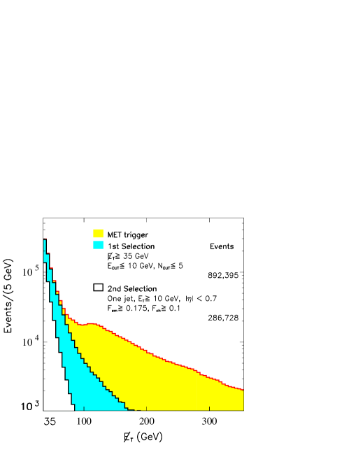
  Figure 2: The $E{\!\!\!\!}/_{T}$ spectrum after the online trigger and the two stages of the data preselection. The numbers of events surviving the first and second selections are 892,395 and 286,728, respectively. The variables $E_{OUT},~{}N_{OUT}$ are energy and number of towers out of time [17].

• The $W$ and $Z$ boson QCD associated production background estimate. As mentioned, the $Z(\rightarrow e^{+}e^{-})+jets$ data sample is used as standardizable candle to normalize the theoretical rate predictions. The sample used is the events selected from a high energy electron trigger that have a second electron and the invariant mass of the the two is consistent with the Z mass as shown in Figure  4. Exactly the same selection rules and corrections are applied in the data and Monte Carlo samples.

  

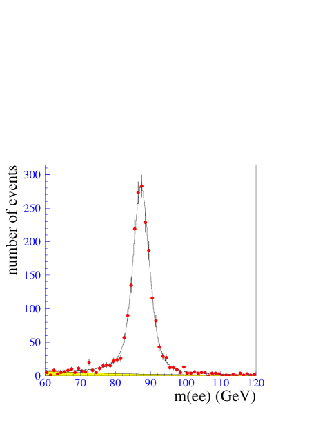
  Figure 3: The $Z^{0}$ mass as reconstructed in the mode $Z^{0}\rightarrow e^{+}e^{-}$ by the DØ detector. The shaded region at the bottom of the plot is the background contribution. The peak does not fall exactly on the true value of $M_{Z}$ because not all of the energy corrections have been applied to the data. This is why it is referred to in the text as a standardizable candle; After the appropriate corrections are made the events in the Z boson mass peak are used for the normalization of the the vector boson+jets rates. The histogram is the prediction and the points the DØ data.

• The multijet QCD production background estimate. The JET data samples are used to normalize the theoretical rate prediction. The source of missing energy in QCD jet production is the small fraction of $b\bar{b}$ and $c\bar{c}$ content (with the $b$ and $c$ quarks decaying semileptonically) and largely the jet mismeasurements and detector resolution. Analyses that require a measurement of the QCD multijet background use the jet data when there are extra requirements such as a $b$-tagged jet or a lepton. The data give a reliable estimate for the QCD background in such analyses. Comparisons between data and herwig QCD Monte Carlo for the $\Sigma\mbox{$E_{T}$}$ cross section measurement at CDF indicate agreement between the data and the Monte Carlo predictions. In the case of the large missing energy plus multijet ($\geq 3$ jets) search the estimate of the QCD background is nontrivial. The missing energy trigger accepts QCD multijet events (45% of the online missing energy trigger are volunteers from jet triggers) and the trigger threshold is too high to allow use of the low missing energy triggered data for extraction of the high missing energy spectrum. The high energy threshold jet triggered data with small or no prescale (JET70, JET100) are not suitable to extract the QCD contribution to the high $E{\!\!\!\!}/_{T}$  tails as they themselves constitute signal candidate samples. The lower energy threshold jet triggered data with large prescales (JET20, JET50) are used in this analysis to estimate the QCD jet production contribution to the high missing energy spectrum. Large statistics 3-jet QCD Monte Carlo samples are generated to simulate the JET20 and JET50 data samples and used to compare the shapes of the missing energy and the $N$-jet distribution with the data. The predictions are absolutely normalized to the data.

• The comparisons of the total background estimates with the data in the control regions around the Blind Box.

  There are seven control regions around the blind box formed by inverting the requirements which define it. We compare the Standard Model background predictions in the control regions with the data. The results are shown in Table  3.

  Region Definition	EWK	QCD	All	Data
  $E{\!\!\!\!}/_{T}$ $\geq$70,$H_{T}$$\geq$150,$N_{trk}^{iso}$$>0$	14	6.3	20$\pm$5	10
  $E{\!\!\!\!}/_{T}$ $\geq$70,$H_{T}$$<$150,$N_{trk}^{iso}$$=0$	2.3	6.3	8.6$\pm$4.5	12
  35$<$$E{\!\!\!\!}/_{T}$ $<$70,$H_{T}$$>$150,$N_{trk}^{iso}$$=0$	1.95	135	137$\pm$28	134
  $E{\!\!\!\!}/_{T}$ $>$70,$H_{T}$$<$150,$N_{trk}^{iso}$$>0$	1.7	$<$0.1	1.7$\pm$0.3	2
  35$<$$E{\!\!\!\!}/_{T}$ $<$70,$H_{T}$$>$150,$N_{trk}^{iso}$$>0$	14	9.4	23$\pm$6	24
  35$<$$E{\!\!\!\!}/_{T}$ $<$70,$H_{T}$$<$150,$N_{trk}^{iso}$$=0$	5	413	418$\pm$69	410
  35$<$$E{\!\!\!\!}/_{T}$ $<$70,$H_{T}$$<$150,$N_{trk}^{iso}$$>0$	3.3	28	31$\pm$10	35
  Signal Candidate Region
  $E{\!\!\!\!}/_{T}$ $\geq$70,$H_{T}$$\geq$150,$N_{trk}^{iso}$$=0$	35	41	76$\pm$13	74

  Table 3: Comparison of the  Standard Model prediction and the data in the control regions and the signal candidate region (blind box). After the contents of the control regions were compared in detail to standard model predictions, we opened the box and found 74 events. ($E{\!\!\!\!}/_{T}$  and $H_{T}$  in GeV.)

Of the 76 events predicted in the blind box, 41 come from QCD and 35 from electroweak processes. Of the latter we estimate $\sim$37% coming from $Z(\rightarrow\nu\bar{\nu})+\geq 3$ jets, $\sim$20% from $W(\rightarrow\tau\nu)+\geq 2$ jets, $\sim$20% from the combined $W(\rightarrow e(\mu)\nu_{e}(\nu_{\mu}))+\geq 3$ jets, and $\sim$20% from $t\bar{t}$ production and decays. We also compare the kinematic properties between Standard Model predictions and the data around the box and find them to be in agreement  [17].

As we mentioned in the introduction we can stop here and show histograms of how well the data match the Standard Model predictions both in the blind box and in the control regions 4.

Figure 4: Comparison in the blind box between data (points) and Standard Model predictions (histogram) of  $E{\!\!\!\!}/_{T}$, $N_{jet}$, leading jet $E_{T}$ and $H_{T}$ distributions. There are 74 events in each of these plots, to be compared with 76$\pm$13 SM predicted events. Note that the $E{\!\!\!\!}/_{T}$ distribution is plotted with a variable bin size; the bin contents are normalized as labelled.

We can combine the level of agreement in this channel with a number of searches in other final states and make a global analysis of how well all the data in all analyses match the Standard Model predictions. However we choose to take the analysis a step further. We pick two models and provide an answer to a model builder who wants to know how light a gluino is allowed to be based on this particular search. We study the hadroproduction of scalar quarks and gluinos and all their decays in minimal Supersymmetry and Supergravity frameworks. Important theoretical considerations that need to be underlined are a) the use of $\tan\beta=3$ to generate datasets of squark and gluino events, b) the study of the production of only thefirst two heavy generations of squarks ($\tilde{u},\tilde{d},\tilde{c},\tilde{s})$ in the general MSSM framework while in mSUGRA the production of the bottom squark ($\tilde{b}$) is also considered. Work which is now underway shows that the results are valid also for $\tan\beta=30$.

Based on the observations, the Standard Model estimates and their uncertainties, and the relative total systematic uncertainty on the signal efficiency, we derive the 95% C.L. upper limit on the number of signal events. The bound is shown on the $\mbox{$m_{\widetilde{q}}$}-\mbox{$m_{\widetilde{g}}$}$ plane in Figure 3. For the signal points generated with mSUGRA, the limit is also interpreted in the $M_{0}-M_{1/2}$ plane  [17].

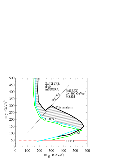
Figure 5: The 95% C.L. limit curve in the $\mbox{$m_{\widetilde{q}}$}~{}-~{}\mbox{$m_{\widetilde{g}}$}$ plane for $\tan\beta=3$; the hatched area is newly excluded by this analysis. Results from some previous searches are also shown.

4.1.1 What did we learn?

We learned that there is no excess of multijet events at the tails of the missing energy distribution in 84 pb^-1 of data. We learned that we can simulate well the tails of the missing energy adequately for 84 pb^-1 of data and predict the standard model backgrounds robustly. We learn that the LEP results are in accord with the Tevatron results when we both consider a minimal supersymmetric model. And we learn that the scale of SUSY can still be the electroweak scale. Lets discuss the latter a bit more.

The notion of naturalness and fine-tuning  [18] is not extremely well defined, but it is used unavoidably since it is the fine-tuning in the Standard Model  that motivates low-energy supersymmetry and supports the projection that superpartners should be found before or at the LHC. Many measures and studies of fine-tuning have appeared in the literature  [19, 20, 21, 22, 23].

In a model-independent analysis  [24], naturalness constraints are weak for some superpartners, e.g. the squarks and sleptons of the first two generations. In widely considered scenarios with scalar mass unification at a high scale, such as minimal supergravity, it is assumed that the squark and slepton masses must be $\mathrel{\hbox to0.0pt{\raise 2.15277pt\hbox{$<$}\hss}{\lower 2.15277pt\hbox{$\sim$}}}$1 TeV/$c^{2}$. This bound places all scalar superpartners within the reach of present and near future colliders. This assumption is re-examined  [23] in models with strong unification constraints, and the squarks and sleptons are found to be natural even with masses above 1 TeV/$c^{2}$. Furthermore by relaxing the universality constraints the naturalness upper limits on supersymmetric particles increase significantly  [20] without extreme fine-tuning. This suppresses sparticle mediated rare processes and the problem of SUSY flavor violations is ameliorated. The fine-tuning due to the chargino mass is found to be model dependent  [22]. With or without universality constraints the gluino remains below 400 GeV/$c^{2}$  [20]. In fact, as it is pointed in  [22] the tightest constraints on fine-tuning come from the experimental limits on the lightest CP-even Higgs boson and the gluino for a number of supersymmetry models. It is then those two key particles that are within reach of the Tevatron collider. These results follow from the observation that fine-tuning is mainly dominated by $M_{3}$, the gluino mass parameter at the electroweak scale, and this dominant contribution can be partly canceled by negative contributions from other soft parameters, as can be seen from the expansion of the $Z$ mass in terms of the input parameters (and for fixed $\tan\beta=2.5$) [22] :

$$M_{Z}^{2}=-1.7\mu^{2}(0)~{}+~{}7.2M_{3}^{2}(0)~{}-0.24M_{2}^{2}(0)~{}+~{}0.014M_{1}^{2}(0)+...$$

The required cancellation is easier if $M_{3}(0)(\sim\mbox{$m_{\widetilde{g}}$})$ is not large (or alternatively if $M_{2}$ is increased for a given $M_{3}$). Using the results of this analysis on the gluino mass we get:

$$M_{3}\mathrel{\hbox to0.0pt{\raise 2.15277pt\hbox{$>$}\hss}{\lower 2.15277pt\hbox{$\sim$}}}300\rightarrow\frac{7.2M_{3}^{2}}{M_{Z}^{2}}\mathrel{\hbox to0.0pt{\raise 2.15277pt\hbox{$>$}\hss}{\lower 2.15277pt\hbox{$\sim$}}}80$$

A similar relation is derived using the LEP limits on the chargino $m_{\widetilde{\chi}_{1}^{+}}\mathrel{\hbox to0.0pt{\raise 2.15277pt\hbox{$>$}\hss}{\lower 2.15277pt\hbox{$\sim$}}}100$ GeV/$c^{2}$  [25, 26, 27] that points to the consideration of gaugino mass non-unification with a lighter gluino. The main effect of a relatively light gluino is the enhancement of the missing energy plus multijet signal with a lepton veto, since for a given chargino mass not yet excluded, the $\widetilde{g}\widetilde{g}$ cross section is enhanced and the gluino cascade decays through charginos are suppressed (fewer leptons are produced in the final state [28, 29]).

4.1.2 The $E{\!\!\!\!}/_{T}$  trigger

The $E{\!\!\!\!}/_{T}$ trigger drives a number of analyses a few of which are the following:

• Vector boson production and leptonic decays. Although there is a dedicated $E{\!\!\!\!}/_{T}$ plus lepton trigger for the study of the $W$ boson, $W$ QCD associated production remains a crucial background for a number of searches beyond the Standard Model and the $E{\!\!\!\!}/_{T}$  plus jets trigger provides a good sample to study these processes. For $Z$ production and decay, the $E{\!\!\!\!}/_{T}$ sample provides a dataset to measure directly the $Z\to\nu\bar{\nu}$ + jets cross section. Furthermore again, the $Z$ boson QCD associated production is a background to many searches.

• top quark production and decay to a $W+b$. The $E{\!\!\!\!}/_{T}$ trigger provides an alternate dataset to measure the top cross section.

• Associated Higgs-$W$ and Higgs-$Z$ production. The $E{\!\!\!\!}/_{T}$ combined with a b quark tagging or a tau lepton tagging trigger can provide a highly efficient triggering scheme for the discovery of the Higgs boson.

• Beyond the Standard Model  searches. To mention a few, the $E{\!\!\!\!}/_{T}$ trigger can be used to search for:

  • Supersymmetric partners: In R-Parity conserving supersymmetric scenarios the LSP (Lightest Supersymmetric Particle) escapes the detector and appears as energy imbalance. Examples are squark and gluino searches, scalar top and scalar bottom quark (utilizing an additional heavy flavor tag) searches. In gauge mediated supersymmetry breaking scenarios that incorporate gravity the LSP is the gravitino – the spin 3/2 partner of the graviton. The gravitino goes undetected and produces energy imbalance.

  • Leptoquarks: The leptoquark decays to a quark and a neutrino resulting in large $E{\!\!\!\!}/_{T}$.

  • CHArged Massive Particles (CHAMPS): These are long-lived massive particles that if they are penetrating enough can go undetected and cause energy imbalance.

  • Gravitons: In braneworld theories of extra dimensions  [30, 33] the graviton can be produced in high energy hadron collisions and escapes to the extra spatial dimensions resulting in energy imbalance.

The specifications of the $E{\!\!\!\!}/_{T}$ trigger acquiring RUNII data was determined using the Run 1B data and the main feature of the trigger is the lower Level 2 $E{\!\!\!\!}/_{T}$ threshold (25 GeV, compared to 35 GeV in Run 1B).

4.2 Example 2: Monojets and missing energy: Looking for KK graviton emission

By now you know exactly the steps of how to do this analysis: you need the clean $E{\!\!\!\!}/_{T}$ triggered data sample and orthogonal data samples to normalize your background estimates, so that your uncertainties in the standard model predictions are dominated by the data statistics and not by systematics.

4.2.1 On the theory

It has been discussed since 1996  [31] that weak scale superstrings have experimental consequences in collider physics. The missing energy as a signature was discussed already in  [32]. Consider the braneworld scenario where gravity propagates in the $4+n$ dimensional bulk of spacetime, while the rest of the standard model fields are confined to the 3+1 dimensional brane. Assume compactification of the extra $n$ dimensions on a torus with a common scale $R$, and identify the massive Kaluza-Klein (KK) states in the four-dimensional spacetime. In such a model, the Planck scale $M_{Pl}$, the compactification scale $R$, and the new effective Planck scale $M_{D}$, are related by the expression:

$$M_{Pl}^{2}\sim R^{n}M^{2+n}_{D}$$

where $n$ is the number of extra dimensions.

Searches for extra dimensions at colliders focus on the search for the emission of gravitons or the effects of the exchange of virtual gravitons (see J. Hewett, this school proceedings). Here we focus on a search for graviton emission.

There are three processes which can result in the emission of gravitons:

• $q\overline{q}\rightarrow gG$

• $qg\rightarrow qG$

• $gg\rightarrow gG$

where $G$ is the graviton. The Feynman diagrams for these processes are shown in Figure 6.

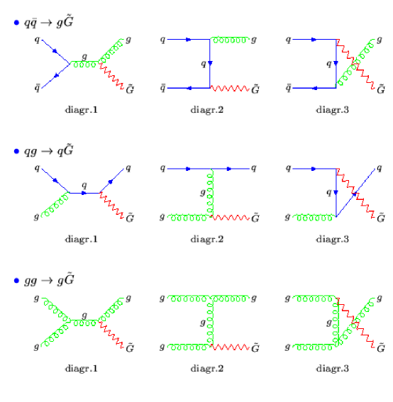
Figure 6: Feynman diagrams for the emission of real gravitons in $p\overline{p}$ collisions. Top: $q\overline{q}\rightarrow gG$. Middle: $qg\rightarrow qG$. Bottom: $gg\rightarrow gG$.

In all three cases the signature will be jets + $E{\!\!\!\!}/_{T}$. We included in pythia these processes using the large toroidal extra dimensions model of Arkani-Hamed, Dimopoulos, and Dvali [33], and the calculations of Giudice, Rattazzi, and Wells [34].

The differential cross-sections for the parton processes relevant to graviton plus jet production in hadron collisions are given in Equations 3, 4, and 5.

$$\frac{d^{2}\sigma}{dt~{}dm}(q\bar{q}\to gG)=\frac{\alpha_{s}}{36}~{}\frac{2\pi^{n/2}}{\Gamma(n/2)}~{}\frac{1}{s\mbox{$M_{D}$}^{2+n}}~{}m^{n-1}~{}F_{1}(t/s,m^{2}/s),$$ (3)

$$\frac{d^{2}\sigma}{dt~{}dm}(qg\to qG)=\frac{\alpha_{s}}{96}~{}\frac{2\pi^{n/2}}{\Gamma(n/2)}~{}\frac{1}{s\mbox{$M_{D}$}^{2+n}}~{}m^{n-1}~{}F_{2}(t/s,m^{2}/s),$$ (4)

$$\frac{d^{2}\sigma}{dt~{}dm}(gg\to gG)=\frac{3\alpha_{s}}{16}~{}\frac{2\pi^{n/2}}{\Gamma(n/2)}~{}\frac{1}{s\mbox{$M_{D}$}^{2+n}}~{}m^{n-1}~{}F_{3}(t/s,m^{2}/s)$$ (5)

The Mandelstam variable $t$ in Equations. 3-5 is defined as $t=(p_{q}-p_{G})^{2}$.

The calculation of graviton emission is based on an effective low-energy theory that is valid at parton energies below the scale $M_{D}$.

The $F_{i}(x,y)$ functions in Equations 3-5 are

$$F_{1}(x,y) = \frac{1}{x(y-1-x)}\left[-4x(1+x)(1+2x+2x^{2})+\right.$$ (6)

$$\left.y(1+6x+18x^{2}+16x^{3})-6y^{2}x(1+2x)+y^{3}(1+4x)\right],$$

$$F_{2}(x,y) = -(y-1-x)~{}F_{1}\left(\frac{x}{y-1-x},\frac{y}{y-1-x}\right)=$$ (7)

$$\frac{1}{x(y-1-x)}\left[-4x(1+x^{2})+y(1+x)(1+8x+x^{2})\right.$$

$$\left.-3y^{2}(1+4x+x^{2})+4y^{3}(1+x)-2y^{4}\right],$$

$$F_{3}(x,y)= \frac{1}{x(y-1-x)}\left[1+2x+3x^{2}+2x^{3}+x^{4}\right.$$ (8)

$$\left.-2y(1+x^{3})+3y^{2}(1+x^{2})-2y^{3}(1+x)+y^{4}\right].$$

The function $F_{1}(x,y)$ determines the cross-section for $f\bar{f}\to\gamma G$. $F_{1}(x,y)$ is invariant under exchange of the Mandelstam variables $t$ and $u$; this is reflected in the property $F_{1}(x,y)=F_{1}(y-1-x,y)$. The same property holds also for the function $F_{3}(x,y)$, relevant to the QCD process.

Cross sections from pythia for individual graviton production sub-processes are shown as a function of $M_{D}$ for different values of $n$ in Figures 7 and  8. Figure 7 compares the different sub-processes for the same value of $n$, while Figure 8 compares different values of $n$ for the same sub-process.

Note that the cross-section for $q\bar{q}\to gG$ is larger for larger values of $n$, relative to the other sub-processes. This can be traced to the different dependences of $F_{1},\ F_{2},$ and $F_{3}$ on $m^{2}/s$ (labelled $y$ in equations 6-8). $F_{2}$ and $F_{3}$ have a dependence on quartic dependence on $y$, whereas $F_{1}$ has only a cubic dependence. This results in larger splittings at high values of $M_{D}$ between different values of $n$ for $qg\to qG$ and $gg\to gG$ compared to $q\bar{q}\to gG$.

Figure 7: Cross sections for each subprocess for (a) n=2, (b) n=4, and (c) n=6.

Figure 8: Cross sections for n=2, 4, and 6, for each subprocess: (a) $q\bar{q}\to gG$ (b) $qg\to qG$, and (c) $gg\to gG$.

For $M_{D}$ = 1 TeV a significant number of heavy KK gravitons will be produced with masses averaging in the hundreds of GeV, as can be seen in Fig. 9. The peak of the mass distribution is higher for $n=6$ extra dimensions, because the density of KK states is a more rapidly increasing function than for $n=2$. This difference does not show up in the $E{\!\!\!\!}/_{T}$ distribution (Fig. 9). This is due to two competing effects: (1) the heavier KK gravitons for $n=6$ have larger transverse energy, but (2) the rapidly decreasing parton distribution functions cause the heavier gravitons to be produced near threshold. These two effects cancel, leaving nearly identical $E{\!\!\!\!}/_{T}$ distributions for different values of $n$.

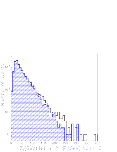
Figure 9: (l)The graviton mass distribution for $n=2$ and $n=6$ extra dimensions. (r) The $E{\!\!\!\!}/_{T}$ distribution for n=2 and $n=6$ extra dimensions(shaded) for $qg\to qG$ process simulation.

4.2.2 The Analysis

The data preselection and the jet fiducial requirements are the same as in the case of the multijet plus $E{\!\!\!\!}/_{T}$ analysis used in the search for gluinos and squarks and they are designed to retain a high purity in the real missing energy sample.

In the missing energy plus one jet search, the missing energy comes from the KK graviton tower and the one jet from the recoiling parton. To reduce the background contribution from $W\rightarrow\ell\nu$+jets we apply the same indirect lepton veto as in the multijet analysis.

To define the signal region we use three variables: the $E{\!\!\!\!}/_{T}$ , the $N_{jet}$ and the Isolated Track Multiplicity $N_{trk}^{iso}$. The requirements are, no isolated tracks, large missing energy and one or two jets (when two the second must not be grossly mismeasured).

The value of the missing energy requirement for the definition of the graviton signal region is driven by the missing energy Level 2 trigger efficiency and optimized for the graviton signal. The $N_{jet}$ requirement is motivated by the graviton monojet signal characteristic final state. The second jet is primarily allowed so that the QCD background can be calculated using the HERWIG Monte Carlo and the CDF detector simulation with a reliable normalization from the CDF QCD data, and additionally so that the systematic uncertainty of the signal due to ISR/FSR is kept as low as possible. Allowing a second jet also permits interpretation of the results with a k-factor inclusion in the signal cross section estimate.

The $N_{trk}^{iso}$  requirement increases the sensitivity to the graviton signal by reducing the $W$+jet contribution, while at the same time retaining the signal. The rest of the analysis path is based on the kinematics and aims at high sensitivity for the signal.

4.2.3 Summary of Standard Model  processes with
$\mbox{$E{\!\!\!\!}/_{T}$}~{}+$ jet in the final state

The Standard Model processes with large missing energy and multijets in the final state that constitute backgrounds to the graviton search are

• $Z$+jets : QCD associated $Z$ production with $Z\rightarrow\nu\nu$ is the most significant and irreducible background component. For the $Z+$jets backgrounds the pythia  Monte Carlo simulation is used and normalized to the $\mbox{$Z\rightarrow\ ee$}+\geq 1$ jet data (our standardizable candle).

• $W+$jets : QCD associated $W$ production with $W\rightarrow\ e\nu$, $W\rightarrow\ \mu\nu$, and $W\rightarrow\ \tau\nu$ has a large $E{\!\!\!\!}/_{T}$  + jet contribution. For the $W+$jets and backgrounds the pythia  Monte Carlo simulation is used and normalized using the $\mbox{$Z\rightarrow\ ee$}+\geq 1$ jet data sample.

• top, single top : In $t\bar{t}$ production a $W$ from a top decay can decay semileptonicaly and contribute to the high $E{\!\!\!\!}/_{T}$  tails. We use pythia  to simulate $t\bar{t}$  production with all inclusive top decays. For the normalization to the data luminosity the theoretical calculation $\sigma(t\bar{t})=5.1~{}{\rm}pb~{}\pm~{}18\%$ (which is consistent with the CDF $t\bar{t}$ [45] cross section) is used. herwig  and pythia  Monte Carlo programs are used to simulate single top production via W-gluon fusion and W* production respectively. The theoretical cross sections $\sigma(tq^{\prime})=1.7~{}{\rm pb}~{}\pm 15\%$ and $\sigma(bt)=0.73~{}{\rm pb}~{}\pm 9\%$  [45] are used to normalize the samples.

• dibosons : For $WW$, $WZ$, $ZZ$ production pythia is used. For the normalization, the theoretical cross sections calculated for each diboson process are used: $\sigma(WW)=9.5\pm 0.7~{}{\rm pb},~{}\sigma(WZ)=2.6\pm 0.3~{}{\rm pb}$ and $\sigma(ZZ)=1\pm 0.2~{}{\rm pb}$  [45] are used.

• QCD : The QCD background is generated with herwig  and normalized to the CDF jet data using dijet events. Clearly one does not expect this to be a significant physics background.

Once the signal to background ratio is optimized as a function of the measured variables (kinematical,topological etc), the requirements are set and the data are compared to the standard model predictions. From there of course we can interprete the results as a limit in the allowable cross section of non-standard model processes, extra dimensions and what not. The result of this particular analysis has been reported in conferences and will appear soon in the literature but similar analyses from CDF and D0 have already reported results [47].

5 What next?

It is a very interesting time for physics, indeed for fundamental physics. Recent experimental cosmology results are changing the ideas we had about how much of the universe we know and how well. Results in particle physics, such as the massiveness of the neutrinos, the tremendous precision at which the Standard Model holds in the up to now explored electroweak scale region (without the Higgs boson showing up), are all puzzling us. Putting together a picture of how spacetime happens and how it is filled, by means of observations and studies in a controlled experimental environment, is the primary and urgent work of both experimentalists and theorists. In these lectures I gave examples of how we go about this using colliders.

Many thanks to the school organizers Joe Lykken, Steve Gubser, and Kalyana T. Mahanthappa; the TASI 2001 students; Kevin Burkett and all my CDF collaborators always. The author is supported by NSF and the Pritzker Foundation.

References

- [1] Medical Accelerators in Radiotherapy: Past Present and Future, Physics Medica, Vol. XII N.4, (1996).
-
[2]
U. Amaldi,
http://web.cern.ch/AccelConf/e96/PAPERS/ORALS/FRY01A.PDF] -
[3]
APS News, Backpage, December 2002
http://www.aps.org/apsnews/1202/120213.htm - [4] NLC Design and Physics Working Group, FERMILAB-PUB-96/112, 1996.
- [5] J. Polchinski, arXiv:hep-th/9607050 (1996).
- [6] http://hep.uchicago.edu/cdf/smaria/ms/aaas03.html
- [7] e.g. Pierre Ramond, Phys. Rev. D3, 2415, (1971).
- [8] G. Kane, Supersymmetry, Perseus Books, (2000)
- [9] P. Drell, hep-ex/9701001, (1997).
- [10] R. Markeloff, University of Winsconsin, Ph.D. thesis, (1994).
- [11] The D0 Collaboration, Phys. Rev. Lett. 79, 1203, (1997).
- [12] T. Affolder et al., The CDF Collaboration, to be submitted.
- [13] T. Affolder et al., The CDF Collaboration, Phys. Rev. Lett. 85, 5704, (2000).
- [14] T. Affolder et al., The CDF Collaboration, Phys. Rev. Lett. 85, 1378 (2000).
- [15] T. Affolder et al., The CDF Collaboration, FERMILAB-PUB-00/073-E, submitted to Phys. Rev. Lett. March 31, (2000).
- [16] is the number of high momentum isolated tracks in the event. Tracks qualify as such if they have transverse momentum 10 GeV/, impact parameter , vertex difference cm and the total transverse momentum of all tracks (with impact parameter cm) around them in a cone of is .
- [17] M. Spiropulu, Harvard University Ph.D thesis (2000); T. Affolder et al. The CDF Collaboration,Phys. Rev. Lett. 88, 241802 (2002).
-
[18]
E. Gildener,
Phys. Rev. D14, 1667, (1976);
E.Gildener and S. Weinberg, Phys. Rev. D13, 3333, (1976);
L. Maiani, Proceedings of the Summer School of Gif-Sur-Yvette (1980);
M. Veltman, Acta Phys. Polon. B12, 437, (1981);
S. Dimopoulos and S. Raby, Nucl. Phys. B192, 353, (1981);
E. Witten, Nucl. Phys. B188, 513, (1981);
S. Dimopoulos and H. Georgi Nucl. Phys. B193, 150, (1981). - [19] R. Barbieri and G.F. Giudice, Nucl. Phys. B306 63, (1988).
- [20] S. Dimopoulos and G.F. Giudice, Phys. Lett. B357, 573, (1995).
- [21] G. Anderson and D. Castano, Phys.Rev. D52, 1693, (1995).
- [22] M. Bastero-Gil, G. L. Kane and S. F. King Phys. Lett. B 474, 103 (2000); G. L. Kane and S .F. King, Phys. Lett. B451 113, (1999), and references therein.
-
[23]
J.L. Feng, K.T. Matchev and T. Moroi,
Proceedings of PASCOS’99, Lake Tahoe, December 10-16, 1999;
J.L. Feng, K.T. Matchev and T. Moroi, Phys. Rev. Lett. 84 2322, (2000);
J. Bagger, J. Feng, N. Polonsky, Nucl. Phys. B563, 3, (1999). - [24] S. Coleman and D.J. Gross, Phys. Rev. Lett. 31, 851, (1973).
- [25] S. Rosier-Lees, LEP SUSY Working Group Status Report, LEPC, http://lepsusy.web.cern.ch/lepsusy/, (2000).
- [26] S. Martin, DPF, http://www.dpf2000.org/BSM1.htm#ses1 (2000).
- [27] G. L. Kane, J. Lykken, B. D. Nelson and L. T. Wang, Phys. Lett. B 551, 146 (2003).
- [28] V. Barger, C. E. M. Wagner, et al. hep-ph/0003154, (2000).
- [29] G. Anderson, H. Baer, C. Chen and X. Tata, Phys. Rev. D61, 095005, (2000)
- [30] G. Nordstrom, Z. Phys. 15, 504 (1914); T. Kaluza, Preuss. Akad. Wiss, Berlin, Math. Phys. K 1, 966 (1921); O. Klein Z. Phys. 37 895; Nature 118, 516 (1926).
- [31] J. D. Lykken, Phys. Rev. D 54, 3693 (1996)
- [32] I. Antoniadis, N. Arkani-Hamed, S. Dimopoulos and G. R. Dvali, Phys. Lett. B 436, 257 (1998)
- [33] N. Arkani-Hamed, S. Dimopoulos and G. R. Dvali, Phys. Lett. B 429, 263 (1998)
- [34] G. F. Giudice, R. Rattazzi and J. D. Wells, Nucl. Phys. B 544, 3 (1999) [arXiv:hep-ph/9811291].
- [35] T. Han, J. D. Lykken and R. J. Zhang, Phys. Rev. D 59, 105006 (1999) [arXiv:hep-ph/9811350].
- [36] For a review, see J. Hewett and M. Spiropulu Annu. Rev. Nucl. Part. Sci., Vol. 52: 397-424 (2002).
- [37] T. Sjöstrand, Comput. Phys. Commun. 82, 74 (1994). pythia v6.115 is used.
- [38] F. Abe et al., Nucl. Inst. and Methods, A271, 387 (1988).
- [39] In the CDF coordinate system, and are the azimuthal and polar angles with respect to the proton beam direction. The pseudorapidity is defined as .
- [40] F. Abe et al., The CDF Collaboration, Phys. Rev. D45, 1448 (1992).
- [41] If there are multiple vertices in the event we use the vertex with the largest of associated tracks.
- [42] T. Affolder et al. The CDF Collaboration, Phys. Rev. Lett. 88, 241802 (2002).
- [43] is the number of high momentum isolated tracks in the event. Tracks qualify as such if they have transverse momentum 10 GeV/, impact parameter , vertex difference cm and the total transverse momentum of all tracks (with impact parameter cm) around them in a cone of is .
- [44] G. Marchesini et al., Comput. Phys. Commun. 67, 465 (1992). herwig v5.6 is used. See hep-ph/9607393 (1996).
- [45] R. Bonciani et al., Nucl. Phys. B529, 424 (1998); T. Stelzer, Z. Sullivan and S. Willenbrock, Phys. Rev. D54, 6696 (1996); T. Tait and C. P. Yuan, hep-ph/9710372 (1997); J. Ohnemus et al., Phys. Rev. D43, 3626 (1991); Phys. Rev. D44, 1403 and 3477 (1991). The measured top cross section (T. Affolder et al., Phys. Rev. D64 032002 (2001)) is in agreement with the theoretical prediction.
- [46] G. Zech, Nucl. Instrum. Methods A277, 608 (1989); T.Huber et al ., Phys Rev D41, 2709 (1990).
- [47] Recently the D0 collaboration (arXiv:hep-ex/0302014) reported their limit on direct graviton emission using a -factor of 1.3 in the signal cross-section; D. Acosta et al., The CDF Collaboration, Phys. Rev. Lett. 89 281801 (2002); For a summary of LEP results on graviton emission, see G. Landsberg, arXiv:hep-ex/0105039 (2000).