CERN–EP/2003-008

11 February 2003

DELPHI Collaboration

Abstract

These final results from DELPHI searches for the Standard Model (SM) Higgs boson, together with benchmark scans of the Minimal Supersymmetric Standard Model (MSSM) neutral Higgs bosons, used data taken at centre-of-mass energies between 200 and 209 ${\mathrm{GeV}}$ with a total integrated luminosity of 224 pb^-1. The data from 192 to 202 ${\mathrm{GeV}}$ are reanalysed with improved b-tagging for MSSM final states decaying to four b-quarks. The 95% confidence level lower mass bound on the Standard Model Higgs boson is 114.1 ${\mathrm{GeV}}/c^{2}$. Limits are also given on the lightest scalar and pseudo-scalar Higgs bosons of the MSSM.

(Eur. Phys. J. C32 (2004) 145-183)

J.Abdallah${}^{\ref{LPNHE}}$, P.Abreu${}^{\ref{LIP}}$, W.Adam${}^{\ref{VIENNA}}$, P.Adzic${}^{\ref{DEMOKRITOS}}$, T.Albrecht${}^{\ref{KARLSRUHE}}$, T.Alderweireld${}^{\ref{AIM}}$, R.Alemany-Fernandez${}^{\ref{CERN}}$, T.Allmendinger${}^{\ref{KARLSRUHE}}$, P.P.Allport${}^{\ref{LIVERPOOL}}$, U.Amaldi${}^{\ref{MILANO2}}$, N.Amapane${}^{\ref{TORINO}}$, S.Amato${}^{\ref{UFRJ}}$, E.Anashkin${}^{\ref{PADOVA}}$, A.Andreazza${}^{\ref{MILANO}}$, S.Andringa${}^{\ref{LIP}}$, N.Anjos${}^{\ref{LIP}}$, P.Antilogus${}^{\ref{LYON}}$, W-D.Apel${}^{\ref{KARLSRUHE}}$, Y.Arnoud${}^{\ref{GRENOBLE}}$, S.Ask${}^{\ref{LUND}}$, B.Asman${}^{\ref{STOCKHOLM}}$, J.E.Augustin${}^{\ref{LPNHE}}$, A.Augustinus${}^{\ref{CERN}}$, P.Baillon${}^{\ref{CERN}}$, A.Ballestrero${}^{\ref{TORINOTH}}$, P.Bambade${}^{\ref{LAL}}$, R.Barbier${}^{\ref{LYON}}$, D.Bardin${}^{\ref{JINR}}$, G.Barker${}^{\ref{KARLSRUHE}}$, A.Baroncelli${}^{\ref{ROMA3}}$, M.Battaglia${}^{\ref{CERN}}$, M.Baubillier${}^{\ref{LPNHE}}$, K-H.Becks${}^{\ref{WUPPERTAL}}$, M.Begalli${}^{\ref{BRASIL}}$, A.Behrmann${}^{\ref{WUPPERTAL}}$, E.Ben-Haim${}^{\ref{LAL}}$, N.Benekos${}^{\ref{NTU-ATHENS}}$, A.Benvenuti${}^{\ref{BOLOGNA}}$, C.Berat${}^{\ref{GRENOBLE}}$, M.Berggren${}^{\ref{LPNHE}}$, L.Berntzon${}^{\ref{STOCKHOLM}}$, D.Bertrand${}^{\ref{AIM}}$, M.Besancon${}^{\ref{SACLAY}}$, N.Besson${}^{\ref{SACLAY}}$, D.Bloch${}^{\ref{CRN}}$, M.Blom${}^{\ref{NIKHEF}}$, M.Bluj${}^{\ref{WARSZAWA}}$, M.Bonesini${}^{\ref{MILANO2}}$, M.Boonekamp${}^{\ref{SACLAY}}$, P.S.L.Booth${}^{\ref{LIVERPOOL}}$, G.Borisov${}^{\ref{LANCASTER}}$, O.Botner${}^{\ref{UPPSALA}}$, B.Bouquet${}^{\ref{LAL}}$, T.J.V.Bowcock${}^{\ref{LIVERPOOL}}$, I.Boyko${}^{\ref{JINR}}$, M.Bracko${}^{\ref{SLOVENIJA}}$, R.Brenner${}^{\ref{UPPSALA}}$, E.Brodet${}^{\ref{OXFORD}}$, P.Bruckman${}^{\ref{KRAKOW1}}$, J.M.Brunet${}^{\ref{CDF}}$, L.Bugge${}^{\ref{OSLO}}$, P.Buschmann${}^{\ref{WUPPERTAL}}$, M.Calvi${}^{\ref{MILANO2}}$, T.Camporesi${}^{\ref{CERN}}$, V.Canale${}^{\ref{ROMA2}}$, F.Carena${}^{\ref{CERN}}$, N.Castro${}^{\ref{LIP}}$, F.Cavallo${}^{\ref{BOLOGNA}}$, M.Chapkin${}^{\ref{SERPUKHOV}}$, Ph.Charpentier${}^{\ref{CERN}}$, P.Checchia${}^{\ref{PADOVA}}$, R.Chierici${}^{\ref{CERN}}$, P.Chliapnikov${}^{\ref{SERPUKHOV}}$, J.Chudoba${}^{\ref{CERN}}$, S.U.Chung${}^{\ref{CERN}}$, K.Cieslik${}^{\ref{KRAKOW1}}$, P.Collins${}^{\ref{CERN}}$, R.Contri${}^{\ref{GENOVA}}$, G.Cosme${}^{\ref{LAL}}$, F.Cossutti${}^{\ref{TU}}$, M.J.Costa${}^{\ref{VALENCIA}}$, B.Crawley${}^{\ref{AMES}}$, D.Crennell${}^{\ref{RAL}}$, J.Cuevas${}^{\ref{OVIEDO}}$, J.D’Hondt${}^{\ref{AIM}}$, J.Dalmau${}^{\ref{STOCKHOLM}}$, T.da Silva${}^{\ref{UFRJ}}$, W.Da Silva${}^{\ref{LPNHE}}$, G.Della Ricca${}^{\ref{TU}}$, A.De Angelis${}^{\ref{TU}}$, W.De Boer${}^{\ref{KARLSRUHE}}$, C.De Clercq${}^{\ref{AIM}}$, B.De Lotto${}^{\ref{TU}}$, N.De Maria${}^{\ref{TORINO}}$, A.De Min${}^{\ref{PADOVA}}$, L.de Paula${}^{\ref{UFRJ}}$, L.Di Ciaccio${}^{\ref{ROMA2}}$, A.Di Simone${}^{\ref{ROMA3}}$, K.Doroba${}^{\ref{WARSZAWA}}$, J.Drees${}^{\ref{WUPPERTAL},\ref{CERN}}$, M.Dris${}^{\ref{NTU-ATHENS}}$, G.Eigen${}^{\ref{BERGEN}}$, T.Ekelof${}^{\ref{UPPSALA}}$, M.Ellert${}^{\ref{UPPSALA}}$, M.Elsing${}^{\ref{CERN}}$, M.C.Espirito Santo${}^{\ref{LIP}}$, G.Fanourakis${}^{\ref{DEMOKRITOS}}$, D.Fassouliotis${}^{\ref{DEMOKRITOS},\ref{ATHENS}}$, M.Feindt${}^{\ref{KARLSRUHE}}$, J.Fernandez${}^{\ref{SANTANDER}}$, A.Ferrer${}^{\ref{VALENCIA}}$, F.Ferro${}^{\ref{GENOVA}}$, U.Flagmeyer${}^{\ref{WUPPERTAL}}$, H.Foeth${}^{\ref{CERN}}$, E.Fokitis${}^{\ref{NTU-ATHENS}}$, F.Fulda-Quenzer${}^{\ref{LAL}}$, J.Fuster${}^{\ref{VALENCIA}}$, M.Gandelman${}^{\ref{UFRJ}}$, C.Garcia${}^{\ref{VALENCIA}}$, Ph.Gavillet${}^{\ref{CERN}}$, E.Gazis${}^{\ref{NTU-ATHENS}}$, R.Gokieli${}^{\ref{CERN},\ref{WARSZAWA}}$, B.Golob${}^{\ref{SLOVENIJA}}$, G.Gomez-Ceballos${}^{\ref{SANTANDER}}$, P.Goncalves${}^{\ref{LIP}}$, E.Graziani${}^{\ref{ROMA3}}$, G.Grosdidier${}^{\ref{LAL}}$, K.Grzelak${}^{\ref{WARSZAWA}}$, J.Guy${}^{\ref{RAL}}$, C.Haag${}^{\ref{KARLSRUHE}}$, A.Hallgren${}^{\ref{UPPSALA}}$, K.Hamacher${}^{\ref{WUPPERTAL}}$, K.Hamilton${}^{\ref{OXFORD}}$, J.Hansen${}^{\ref{OSLO}}$, S.Haug${}^{\ref{OSLO}}$, F.Hauler${}^{\ref{KARLSRUHE}}$, V.Hedberg${}^{\ref{LUND}}$, M.Hennecke${}^{\ref{KARLSRUHE}}$, H.Herr${}^{\ref{CERN}}$, J.Hoffman${}^{\ref{WARSZAWA}}$, S-O.Holmgren${}^{\ref{STOCKHOLM}}$, P.J.Holt${}^{\ref{CERN}}$, M.A.Houlden${}^{\ref{LIVERPOOL}}$, K.Hultqvist${}^{\ref{STOCKHOLM}}$, J.N.Jackson${}^{\ref{LIVERPOOL}}$, G.Jarlskog${}^{\ref{LUND}}$, P.Jarry${}^{\ref{SACLAY}}$, D.Jeans${}^{\ref{OXFORD}}$, E.K.Johansson${}^{\ref{STOCKHOLM}}$, P.D.Johansson${}^{\ref{STOCKHOLM}}$, P.Jonsson${}^{\ref{LYON}}$, C.Joram${}^{\ref{CERN}}$, L.Jungermann${}^{\ref{KARLSRUHE}}$, F.Kapusta${}^{\ref{LPNHE}}$, S.Katsanevas${}^{\ref{LYON}}$, E.Katsoufis${}^{\ref{NTU-ATHENS}}$, G.Kernel${}^{\ref{SLOVENIJA}}$, B.P.Kersevan${}^{\ref{CERN},\ref{SLOVENIJA}}$, A.Kiiskinen${}^{\ref{HELSINKI}}$, B.T.King${}^{\ref{LIVERPOOL}}$, N.J.Kjaer${}^{\ref{CERN}}$, P.Kluit${}^{\ref{NIKHEF}}$, P.Kokkinias${}^{\ref{DEMOKRITOS}}$, C.Kourkoumelis${}^{\ref{ATHENS}}$, O.Kouznetsov${}^{\ref{JINR}}$, Z.Krumstein${}^{\ref{JINR}}$, M.Kucharczyk${}^{\ref{KRAKOW1}}$, J.Lamsa${}^{\ref{AMES}}$, G.Leder${}^{\ref{VIENNA}}$, F.Ledroit${}^{\ref{GRENOBLE}}$, L.Leinonen${}^{\ref{STOCKHOLM}}$, R.Leitner${}^{\ref{NC}}$, J.Lemonne${}^{\ref{AIM}}$, V.Lepeltier${}^{\ref{LAL}}$, T.Lesiak${}^{\ref{KRAKOW1}}$, W.Liebig${}^{\ref{WUPPERTAL}}$, D.Liko${}^{\ref{VIENNA}}$, A.Lipniacka${}^{\ref{STOCKHOLM}}$, J.H.Lopes${}^{\ref{UFRJ}}$, J.M.Lopez${}^{\ref{OVIEDO}}$, D.Loukas${}^{\ref{DEMOKRITOS}}$, P.Lutz${}^{\ref{SACLAY}}$, L.Lyons${}^{\ref{OXFORD}}$, J.MacNaughton${}^{\ref{VIENNA}}$, A.Malek${}^{\ref{WUPPERTAL}}$, S.Maltezos${}^{\ref{NTU-ATHENS}}$, F.Mandl${}^{\ref{VIENNA}}$, J.Marco${}^{\ref{SANTANDER}}$, R.Marco${}^{\ref{SANTANDER}}$, B.Marechal${}^{\ref{UFRJ}}$, M.Margoni${}^{\ref{PADOVA}}$, J-C.Marin${}^{\ref{CERN}}$, C.Mariotti${}^{\ref{CERN}}$, A.Markou${}^{\ref{DEMOKRITOS}}$, C.Martinez-Rivero${}^{\ref{SANTANDER}}$, J.Masik${}^{\ref{FZU}}$, N.Mastroyiannopoulos${}^{\ref{DEMOKRITOS}}$, F.Matorras${}^{\ref{SANTANDER}}$, C.Matteuzzi${}^{\ref{MILANO2}}$, F.Mazzucato${}^{\ref{PADOVA}}$, M.Mazzucato${}^{\ref{PADOVA}}$, R.Mc Nulty${}^{\ref{LIVERPOOL}}$, C.Meroni${}^{\ref{MILANO}}$, W.T.Meyer${}^{\ref{AMES}}$, E.Migliore${}^{\ref{TORINO}}$, W.Mitaroff${}^{\ref{VIENNA}}$, U.Mjoernmark${}^{\ref{LUND}}$, T.Moa${}^{\ref{STOCKHOLM}}$, M.Moch${}^{\ref{KARLSRUHE}}$, K.Moenig${}^{\ref{CERN},\ref{DESY}}$, R.Monge${}^{\ref{GENOVA}}$, J.Montenegro${}^{\ref{NIKHEF}}$, D.Moraes${}^{\ref{UFRJ}}$, S.Moreno${}^{\ref{LIP}}$, P.Morettini${}^{\ref{GENOVA}}$, U.Mueller${}^{\ref{WUPPERTAL}}$, K.Muenich${}^{\ref{WUPPERTAL}}$, M.Mulders${}^{\ref{NIKHEF}}$, L.Mundim${}^{\ref{BRASIL}}$, W.Murray${}^{\ref{RAL}}$, B.Muryn${}^{\ref{KRAKOW2}}$, G.Myatt${}^{\ref{OXFORD}}$, T.Myklebust${}^{\ref{OSLO}}$, M.Nassiakou${}^{\ref{DEMOKRITOS}}$, F.Navarria${}^{\ref{BOLOGNA}}$, K.Nawrocki${}^{\ref{WARSZAWA}}$, R.Nicolaidou${}^{\ref{SACLAY}}$, M.Nikolenko${}^{\ref{JINR},\ref{CRN}}$, A.Oblakowska-Mucha${}^{\ref{KRAKOW2}}$, V.Obraztsov${}^{\ref{SERPUKHOV}}$, A.Olshevski${}^{\ref{JINR}}$, A.Onofre${}^{\ref{LIP}}$, R.Orava${}^{\ref{HELSINKI}}$, K.Osterberg${}^{\ref{HELSINKI}}$, A.Ouraou${}^{\ref{SACLAY}}$, A.Oyanguren${}^{\ref{VALENCIA}}$, M.Paganoni${}^{\ref{MILANO2}}$, S.Paiano${}^{\ref{BOLOGNA}}$, J.P.Palacios${}^{\ref{LIVERPOOL}}$, H.Palka${}^{\ref{KRAKOW1}}$, Th.D.Papadopoulou${}^{\ref{NTU-ATHENS}}$, L.Pape${}^{\ref{CERN}}$, C.Parkes${}^{\ref{GLASGOW}}$, F.Parodi${}^{\ref{GENOVA}}$, U.Parzefall${}^{\ref{CERN}}$, A.Passeri${}^{\ref{ROMA3}}$, O.Passon${}^{\ref{WUPPERTAL}}$, L.Peralta${}^{\ref{LIP}}$, V.Perepelitsa${}^{\ref{VALENCIA}}$, A.Perrotta${}^{\ref{BOLOGNA}}$, A.Petrolini${}^{\ref{GENOVA}}$, J.Piedra${}^{\ref{SANTANDER}}$, L.Pieri${}^{\ref{ROMA3}}$, F.Pierre${}^{\ref{SACLAY}}$, M.Pimenta${}^{\ref{LIP}}$, E.Piotto${}^{\ref{CERN}}$, T.Podobnik${}^{\ref{SLOVENIJA}}$, V.Poireau${}^{\ref{CERN}}$, M.E.Pol${}^{\ref{BRASIL}}$, G.Polok${}^{\ref{KRAKOW1}}$, P.Poropat^†${}^{\ref{TU}}$, V.Pozdniakov${}^{\ref{JINR}}$, N.Pukhaeva${}^{\ref{AIM},\ref{JINR}}$, A.Pullia${}^{\ref{MILANO2}}$, J.Rames${}^{\ref{FZU}}$, L.Ramler${}^{\ref{KARLSRUHE}}$, A.Read${}^{\ref{OSLO}}$, P.Rebecchi${}^{\ref{CERN}}$, J.Rehn${}^{\ref{KARLSRUHE}}$, D.Reid${}^{\ref{NIKHEF}}$, R.Reinhardt${}^{\ref{WUPPERTAL}}$, P.Renton${}^{\ref{OXFORD}}$, F.Richard${}^{\ref{LAL}}$, J.Ridky${}^{\ref{FZU}}$, M.Rivero${}^{\ref{SANTANDER}}$, D.Rodriguez${}^{\ref{SANTANDER}}$, A.Romero${}^{\ref{TORINO}}$, P.Ronchese${}^{\ref{PADOVA}}$, E.Rosenberg${}^{\ref{AMES}}$, P.Roudeau${}^{\ref{LAL}}$, T.Rovelli${}^{\ref{BOLOGNA}}$, V.Ruhlmann-Kleider${}^{\ref{SACLAY}}$, D.Ryabtchikov${}^{\ref{SERPUKHOV}}$, A.Sadovsky${}^{\ref{JINR}}$, L.Salmi${}^{\ref{HELSINKI}}$, J.Salt${}^{\ref{VALENCIA}}$, A.Savoy-Navarro${}^{\ref{LPNHE}}$, U.Schwickerath${}^{\ref{CERN}}$, A.Segar${}^{\ref{OXFORD}}$, R.Sekulin${}^{\ref{RAL}}$, M.Siebel${}^{\ref{WUPPERTAL}}$, A.Sisakian${}^{\ref{JINR}}$, G.Smadja${}^{\ref{LYON}}$, O.Smirnova${}^{\ref{LUND}}$, A.Sokolov${}^{\ref{SERPUKHOV}}$, A.Sopczak${}^{\ref{LANCASTER}}$, R.Sosnowski${}^{\ref{WARSZAWA}}$, T.Spassov${}^{\ref{CERN}}$, M.Stanitzki${}^{\ref{KARLSRUHE}}$, A.Stocchi${}^{\ref{LAL}}$, J.Strauss${}^{\ref{VIENNA}}$, B.Stugu${}^{\ref{BERGEN}}$, M.Szczekowski${}^{\ref{WARSZAWA}}$, M.Szeptycka${}^{\ref{WARSZAWA}}$, T.Szumlak${}^{\ref{KRAKOW2}}$, T.Tabarelli${}^{\ref{MILANO2}}$, A.C.Taffard${}^{\ref{LIVERPOOL}}$, F.Tegenfeldt${}^{\ref{UPPSALA}}$, J.Timmermans${}^{\ref{NIKHEF}}$, L.Tkatchev${}^{\ref{JINR}}$, M.Tobin${}^{\ref{LIVERPOOL}}$, S.Todorovova${}^{\ref{FZU}}$, B.Tome${}^{\ref{LIP}}$, A.Tonazzo${}^{\ref{MILANO2}}$, P.Tortosa${}^{\ref{VALENCIA}}$, P.Travnicek${}^{\ref{FZU}}$, D.Treille${}^{\ref{CERN}}$, G.Tristram${}^{\ref{CDF}}$, M.Trochimczuk${}^{\ref{WARSZAWA}}$, C.Troncon${}^{\ref{MILANO}}$, M-L.Turluer${}^{\ref{SACLAY}}$, I.A.Tyapkin${}^{\ref{JINR}}$, P.Tyapkin${}^{\ref{JINR}}$, S.Tzamarias${}^{\ref{DEMOKRITOS}}$, V.Uvarov${}^{\ref{SERPUKHOV}}$, G.Valenti${}^{\ref{BOLOGNA}}$, P.Van Dam${}^{\ref{NIKHEF}}$, J.Van Eldik${}^{\ref{CERN}}$, A.Van Lysebetten${}^{\ref{AIM}}$, N.van Remortel${}^{\ref{AIM}}$, I.Van Vulpen${}^{\ref{CERN}}$, G.Vegni${}^{\ref{MILANO}}$, F.Veloso${}^{\ref{LIP}}$, W.Venus${}^{\ref{RAL}}$, F.Verbeure${}^{\ref{AIM}}$, P.Verdier${}^{\ref{LYON}}$, V.Verzi${}^{\ref{ROMA2}}$, D.Vilanova${}^{\ref{SACLAY}}$, L.Vitale${}^{\ref{TU}}$, V.Vrba${}^{\ref{FZU}}$, H.Wahlen${}^{\ref{WUPPERTAL}}$, A.J.Washbrook${}^{\ref{LIVERPOOL}}$, C.Weiser${}^{\ref{KARLSRUHE}}$, D.Wicke${}^{\ref{CERN}}$, J.Wickens${}^{\ref{AIM}}$, G.Wilkinson${}^{\ref{OXFORD}}$, M.Winter${}^{\ref{CRN}}$, M.Witek${}^{\ref{KRAKOW1}}$, O.Yushchenko${}^{\ref{SERPUKHOV}}$, A.Zalewska${}^{\ref{KRAKOW1}}$, P.Zalewski${}^{\ref{WARSZAWA}}$, D.Zavrtanik${}^{\ref{SLOVENIJA}}$, V.Zhuravlov${}^{\ref{JINR}}$, N.I.Zimin${}^{\ref{JINR}}$, A.Zintchenko${}^{\ref{JINR}}$, M.Zupan${}^{\ref{DEMOKRITOS}}$

1 Introduction

This paper presents the final results of the DELPHI collaboration on the search for the Standard Model (SM) Higgs boson, together with benchmark scans of the Minimal Supersymmetric Standard Model (MSSM) neutral Higgs bosons. Results are presented for the SM Higgs particle in the mass range from 12 to 120 ${\mathrm{GeV}}/c^{2}$, and for the A and h bosons of the MSSM in a similar range. With the data taken up to $\sqrt{s}=201.7$ ${\mathrm{GeV}}$, DELPHI excluded a SM Higgs boson with mass from zero to 107.3 ${\mathrm{GeV}}/c^{2}$ [1] at the 95% confidence level. The results obtained for a high mass SM signal with the data taken by DELPHI in the last year of LEP operation, 2000, and analyzed with preliminary calibration constants can be found in Ref. [2]. In that year there was considerable interest caused by the observation of an excess of events when the combined results of all the LEP collaborations were considered  [3]. Results on MSSM Higgs bosons have not previously been published using the DELPHI from the year 2000.

The present work contains a more thorough analysis of the 2000 data, and is combined with the results already published from previous years [1]. It might be compared with the final results on Neutral Higgs bosons from the other LEP collaborations [4]. It benefits from many improvements when compared to the originally published results, including a revised data processing with improved calibrations and significant improvements in the simulation of signal and especially background processes. These analyses concentrate on masses between 105 and 120 ${\mathrm{GeV}}/c^{2}$, but they are also applied to lower masses, down to the ${\mathrm{b}}\bar{\mathrm{b}}$ threshold, in order to derive a constraint on the production cross-section of a SM-like Higgs boson as a function of its mass. The revised data processing and the extension towards low masses implied changes to the analysis selection criteria that were tuned on simulated samples. The high mass optimizations remain the same as in Ref. [2].

The dominant production mechanism at LEP for a scalar Higgs boson, such as the SM predicts, is the s-channel process ${\mathrm{e}}^{+}{\mathrm{e}}^{-}$$\rightarrow\mbox{Z}^{*}\rightarrow$${\mathrm{HZ}}$, but there are additional t-channel diagrams in the H$\nu\bar{\nu}$ and H${\mathrm{e^{+}e^{-}}}$ final states, which proceed through ${\mathrm{W}}^{+}{\mathrm{W}}^{-}$ and ${\mathrm{ZZ}}$ fusions, respectively. In the MSSM, the production of the lightest scalar Higgs boson, h, proceeds through the same processes as in the SM. The data from the search for the SM Higgs boson also provide information on the h boson. However, in the MSSM the production cross-section is smaller than the SM one and can even vanish in certain regions of the MSSM parameter space. There is also a CP-odd pseudo-scalar, A, which would be produced mostly in the ${\mathrm{e}}^{+}{\mathrm{e}}^{-}$$\rightarrow\mbox{Z}^{*}\rightarrow{\mathrm{h}}{\mathrm{A}}$ process at LEP2. This channel is therefore also considered in this paper. For MSSM parameter values for which single h production is suppressed, the associated ${\mathrm{h}}{\mathrm{A}}$ production is enhanced (if kinematically permitted). Previous 95% CL limits from DELPHI on the masses of h and A were 85.9 ${\mathrm{GeV}}/c^{2}$ and 86.5 ${\mathrm{GeV}}/c^{2}$ respectively [1]. The present analysis in the ${\mathrm{h}}{\mathrm{A}}$ channel covers masses between 40 and 100 ${\mathrm{GeV}}/c^{2}$. The MSSM interpretations rely on theoretical calculations with limited second-order radiative corrections. They will be updated in a separate paper using more complete corrections.

In the ${\mathrm{HZ}}$ channel, all known decays of the Z boson (hadrons, charged leptons and neutrinos) have been taken into account, while the analyses have been optimized for decays of the Higgs particle into ${\mathrm{b}}\bar{\mathrm{b}}$, making use of the expected high branching fraction of this mode, and for Higgs boson decays into a pair of $\tau$ particles, which is the second main decay channel in the SM and in most of the MSSM parameter space. The sensitivity of the four-jet search to the decay ${\mathrm{h}}\rightarrow{\mathrm{AA}}$ has been measured and included. The ${\mathrm{h}}{\mathrm{A}}$ production has been searched for in the two main decay channels, namely the ${\mathrm{b}}\bar{\mathrm{b}}$${\mathrm{b}}\bar{\mathrm{b}}$  and ${\mathrm{b}}\bar{\mathrm{b}}\tau^{+}\tau^{-}$ final states. An extended MSSM search, including more signal channels, will be reported separately.

The detector description and the data samples are discussed in section 2, and the simulations with which they are compared are described in section 3. Techniques common to more than one analysis are presented in section 4, while the analyses themselves are described in sections 5 to 9. The systematic errors are discussed in section 10, and the results and conclusions are in sections 11 and 12 respectively.

2 Data samples and detector overview

DELPHI recorded a total of 224 pb^-1 of data in the year 2000.

A short description of the detector can be found in Ref. [5], while more details can be found in Ref. [6, 7] for the original setup and in Ref. [8] for the LEP2 upgrade of the silicon tracking detector.

The whole detector was unchanged from the previous operational period, except that one of the twelve sectors of the Time Projection Chamber (TPC) suffered a failure in September 2000. The reconstruction software for charged particle tracks in data collected after this time was adjusted to make best use of the Silicon Tracker and Inner Detector both placed closer to the beam than the TPC and the Outer Detector and Barrel Rich placed outside the outer radius of the TPC. As a result, the impact of the malfunctioning of that TPC sector on the determination of jet momenta was not large but the ${\mathrm{b}}$-tagging in that twelfth of the detector remained significantly degraded.

LEP was run with a beam energy which was optimized to maximize the sensitivity to the SM Higgs boson. The resulting spectrum is shown in Fig. 1, which also shows seven windows into which the analysis was divided. Data with a beam energy falling into a particular window was treated as if it had the mean energy for that window, giving the values listed in Table 1. These windows were selected to give accurate results without complicating the statistical analysis.

DELPHI recorded 164.1 pb^-1 with a fully operational detector, and 60.1 pb^-1after the TPC problem occurred, as shown in Fig. 1. The analyses described here make a distinction between data collected before and after this event, which are referred to as the first operational period and the second operational period. In the second operational period there were no data in the first two energy windows, resulting in twelve data sets in total. The requirement of adequate detector performance reduces the luminosities in the H${\mathrm{e^{+}e^{-}}}$ and H$\nu\bar{\nu}$ samples by 0.5% and 3.8% respectively in the first period, and 1.7% and 4.3% respectively when the TPC sector was off.

The data have been reprocessed since our previous publication [2]. This reprocessing was primarily motivated by an improved calibration of the TPC.

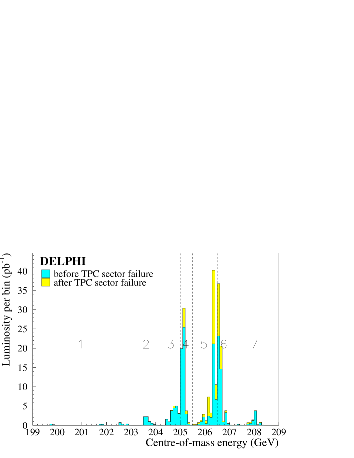
Figure 1: The LEP energy distribution in 2000. The data analysis has been divided into two periods. The darker grey shows the data taken in the first period, and the data taken in the second period is in a lighter grey. The vertical lines and numbers show the energy bins into which the data were grouped.

	Energy windows
Number	1	2	3	4	5	6	7
Low edge, (${\mathrm{GeV}}$)	–	203.0	204.3	205.0	205.5	206.5	207.1
Mean energy, (${\mathrm{GeV}}$)	201.80	203.64	204.73	205.10	206.28	206.59	207.93
Luminosity, (pb-1)	2.92	6.64	19.72	54.97	68.10	62.92	8.91

Table 1: The energy windows into which the recorded data were grouped.

3 Simulation software

The DELPHI simulation software has been significantly upgraded with respect to the version described in Ref. [2]. New Monte Carlo generator software has been used for both two-fermion and four-fermion background processes, and the signal simulations have also been updated. The generated events were passed through the DELPHI detector simulation program [6]. These samples typically correspond to more than 100 times the luminosity of the collected data, with $10^{6}$ hadronic two-fermion and four-fermion background events at each of the following centre of mass energies: 203.7, 205.0, 206.5 and 208.0 ${\mathrm{GeV}}$. Simulated samples allowing estimation of the effect of the TPC problem were also produced at 206.5 ${\mathrm{GeV}}$. Two-fermion background events were generated with KK2f [9] for hadronic events and muon pairs and with KORALZ [10] for $\tau^{+}\tau^{-}$ final states. The four-fermion events, which originate from a coherent sum of many processes whose main components are referred to as $\mbox{Z}\gamma^{*}$, ${\mathrm{W}}^{+}{\mathrm{W}}^{-}$ and ${\mathrm{ZZ}}$ in the following, were generated with WPHACT [11], which includes low-mass hadronic resonances and use of the full CKM matrix. For all of these, the hadronisation was handled by PYTHIA [12], version 6.156.

PYTHIA and BDK [13] with PYTHIA 6.143 fragmentation were used for two-photon processes (hereafter denoted as $\gamma\gamma$) and BHWIDE [14] for Bhabha events in the main acceptance region.

The ZZ production process, especially if at least one of the Z particles decays to b-quarks, is an essentially irreducible background process in all signal channels since it has many features in common with the signal. It is therefore a relevant check on the DELPHI detector that this process can be accurately modelled. This has been demonstrated in Ref. [17].

Signal events were produced using the HZHA [15] generator, which includes the ${\mathrm{W}}^{+}{\mathrm{W}}^{-}$ and ${\mathrm{ZZ}}$ fusion processes in the H$\nu\bar{\nu}$ and H${\mathrm{e^{+}e^{-}}}$ channels respectively, and the interference with HZ. Fragmentation using PYTHIA 6.156 was used to allow for the scalar nature of the Higgs particle, which increases the gluon radiation by some 10% compared with that for a vector boson[16]. For the ${\mathrm{HZ}}$ process, the H mass was varied from 12 to 120 ${\mathrm{GeV}}/c^{2}$, with steps of 5 ${\mathrm{GeV}}/c^{2}$ above 80 ${\mathrm{GeV}}/c^{2}$, and wider steps at lower masses. Extra points were inserted at 114 and 116 ${\mathrm{GeV}}/c^{2}$. For the ${\mathrm{h}}{\mathrm{A}}$ process, samples were generated over a grid of more than 60 points in ($m_{\mathrm{h}}$, $m_{\mathrm{A}}$). Equal mass points were generated from 12 to 100 ${\mathrm{GeV}}/c^{2}$ with a 5 ${\mathrm{GeV}}/c^{2}$ step above 80 ${\mathrm{GeV}}/c^{2}$, and wider steps below. For non-equal ($m_{\mathrm{h}}$, $m_{\mathrm{A}}$) points, the lower mass was varied in the same mass range with a step double that of the equal mass points and, for each of the values of the lower mass, the higher mass was varied up to the kinematic limit with a 20 ${\mathrm{GeV}}/c^{2}$ step. Extra points were generated with a 10 or 5 ${\mathrm{GeV}}/c^{2}$ granularity around 80 ${\mathrm{GeV}}/c^{2}$. In all samples, the Higgs boson widths were set below 1 ${\mathrm{GeV}}/c^{2}$  which is consistent with the expectations of the MSSM in most of the parameter space, that is for $\tan\beta$ (the ratio of the vacuum expectation values of the two Higgs field doublets of the MSSM) below 20. However, for $\tan\beta$ above 20, the h and A widths increase rapidly to reach several ${\mathrm{GeV}}/c^{2}$ at $\tan\beta$ = 50, thus exceeding the experimental mass resolution which is typically around 5 ${\mathrm{GeV}}/c^{2}$ on the sum of the masses in the ${\mathrm{h}}{\mathrm{A}}$ channels. Because of this, a second set of simulations was performed at $\tan\beta$ = 50 with $m_{\mathrm{A}}$ varied according to the same pattern as for the equal mass point simulations. This fixes the h mass, which is almost equal to $m_{\mathrm{A}}$ at such a large value of $\tan\beta$.

The ${\mathrm{HZ}}$ simulated samples were classified according to the Higgs and Z boson decay modes. For H${\mathrm{e^{+}e^{-}}}$, H$\mu^{+}\mu^{-}$ and H$\nu\bar{\nu}$ the natural SM mix of H decay modes into fermions was generated. As final states with hadrons and two $\tau$ particles benefit from a dedicated analysis, the $\tau\tau$ decay mode was removed in the $\mbox{H}{\mathrm{q\bar{q}}}$ channel simulations, and the two ${\mathrm{HZ}}$ channels involving $\tau$ leptons, for which one of the bosons is forced to decay to a $\tau$ pair and the other hadronically, were generated separately. Finally, three sets of ${\mathrm{h}}{\mathrm{A}}$ simulations were generated, covering final states involving either four b-quarks or two b-quarks and two $\tau$ particles, with either the h or the A decaying into two leptons. These were then combined giving equal weight to each channel. Efficiencies were defined relative to these states. The size of these samples was normally 5000 events and they were produced at the same centre-of-mass energies as the background samples.

Although the signal simulations described above cover most of the expected final states in the SM and MSSM, they were complemented by two additional sets at 206.5 ${\mathrm{GeV}}$, one with a fully operational detector and the other one with one TPC sector missing. These samples were of ${\mathrm{h}}{\mathrm{Z}}$  production with ${\mathrm{h}}\rightarrow{\mathrm{AA}}$, as expected in restricted regions of the MSSM parameter space. The A (h) mass was varied from 12 ${\mathrm{GeV}}/c^{2}$ (50 ${\mathrm{GeV}}/c^{2}$) up to the kinematic limit. The final states simulated were hadronic decays of the Z boson and either four b or four c quarks from the A pair. The results obtained from these samples were assumed also to be valid at the other centre-of-mass energies.

4 Features common to all analyses

4.1 Particle selection

In all analyses, charged particles were selected if their momentum was greater than 100 ${\mathrm{MeV}}/c$ and if they originated from the interaction region (within 4 cm in the transverse plane and within 4 cm / $\sin\theta$ along the beam direction, where $\theta$ is the particle polar angle). Neutral particles were defined either as energy clusters in the calorimeters not associated to charged particle tracks, or as reconstructed vertices of photon conversions, interactions of neutral hadrons or decays of neutral particles in the tracking volume. All neutral clusters of energy greater than 200 or 300 ${\mathrm{MeV}}$ (depending on the calorimeter) were used, except in the searches with missing energy, where 300 or 400 ${\mathrm{MeV}}$ was required. The $\pi^{\pm}$ mass was used for all charged particles except identified leptons, while zero mass was used for electromagnetic clusters and the K⁰ mass was assigned to neutral hadronic clusters.

4.2 Jets and Constrained fits

The DURHAM[26] algorithm was used to reconstruct jets, which were taken as estimators of the quark momenta. A constrained fit [20] was performed to reconstruct the Higgs boson mass. The constraints of energy and momentum conservation were applied, and the Z mass was fixed to its central value, except in the H${\mathrm{e^{+}e^{-}}}$ and H$\mu^{+}\mu^{-}$ channels where a Breit-Wigner width was allowed. An algorithm has been developed [21] in order to estimate the effective energy of the ${\mathrm{e}}^{+}{\mathrm{e}}^{-}$ collision. This algorithm makes use of a three-constraint kinematic fit in order to test the presence of an initial state photon along one of the beam directions and hence lost in the beam pipe. This effective centre-of-mass energy is called $\sqrt{s^{\prime}}$ throughout this paper, and is used to remove most of the events radiatively returning to the Z.

4.3 b-quark identification

The method of separation of b-quarks from other flavours is described in detail in Ref. [18], where the various differences between B hadrons and other particles are accumulated into a single variable, hereafter denoted $x_{\mathrm{b}}$ for an event and $x_{\mathrm{b}}^{i}$ for the $i^{th}$ jet of particles. An important contribution to this combined variable is the probability $P_{i}^{+}$ that all tracks with a positive lifetime-signed impact parameter in the jet led to a product of track significances as large as that observed, if these tracks originated from the interaction point; ($P^{+}_{\mathrm{E}}$  is the same, but for all tracks in an event). A low value of this probability is a signature for a B hadron. The likelihood ratio technique was then used to construct $x_{\mathrm{b}}^{i}$ by combining $P_{i}^{+}$ with the transverse momentum (with respect to the jet axis) of any lepton belonging to the jet and with the following information from any secondary vertex found in the jet: the mass computed from the particles assigned to the secondary vertex, the momentum transverse to the line joining the secondary vertex to the primary, the rapidity of the secondary particles, and the fraction of the jet momentum carried by them. The event variable, $x_{\mathrm{b}}$, is $x_{\mathrm{b}}^{1}+x_{\mathrm{b}}^{2}$ for a two jet event, or the sum of the two largest $x_{\mathrm{b}}^{i}$ in the case of a multi-jet configuration. Increasing values of $x_{\mathrm{b}}$ (or $x_{\mathrm{b}}^{i}$) correspond to increasingly ‘b-like’ events (or jets).

Specifically for the four-jet channels, a further improvement of the ${\mathrm{b}}$-tagging procedure was made. The purity of the sample defined by a given b-tagging value had a dependence on various properties of the jet. The ${\mathrm{b}}$-tagging was equalised (see Ref. [18]) to remove this effect explicitly for the following variables: the polar angle of the jet direction, the jet energy, the charged multiplicity of the jet, the angle between the jet direction and the nearest other jet, the average transverse momentum of charged particles with respect to the jet direction, the number of particles with negative impact parameter, and the invariant mass of the jet. Including this dependence in the tagging algorithm significantly improved the rejection of the light quark background events. This technique required specifying the signal hypothesis. For the ${\mathrm{h}}{\mathrm{Z}}$ search this was defined using $m_{\mathrm{h}}$=110 ${\mathrm{GeV}}/c^{2}$ at $\sqrt{s}\,$=206.7 ${\mathrm{GeV}}$, while in the case of ${\mathrm{h}}{\mathrm{A}}$ a mixture of A masses (80 to 95 ${\mathrm{GeV}}/c^{2}$) and beam energies (205 to 208 ${\mathrm{GeV}}$) was used.

The impact parameter resolutions were measured using tracks with negative lifetime signed impact parameters taken from Z calibration events. The overall calibrations were tuned [19] using tracks with negative lifetime signed impact parameters taken from high energy four-jet events. Tuning the Monte Carlo to match the data in this way introduced very little bias as such tracks were only used in the final b-tagging for the equalization corrections described above.

Figure 2: Top: distributions of the combined ${\mathrm{b}}$-tagging variable $x_{\mathrm{b}}$, in events including radiative return to the Z from 2000 data (dots) and simulation (histogram). The contribution of udsc-quarks is shown as the dark histogram. Middle: ratio of integrated tagging rates in 91 ${\mathrm{GeV}}$ Z data and simulation on application of the selection criterion $\mbox{$x_{\mathrm{b}}$}>\mbox{$x_{\mathrm{b}}$}^{\rm cut}$, as a function of the $\mbox{$x_{\mathrm{b}}$}^{\rm cut}$. Bottom: the ratio of the current rate of tagging of Z events to that used in our previous publication, as a function of the cut value $\mbox{$x_{\mathrm{b}}$}^{\rm cut}$. Comparison with the previous processing shows that the efficiency for ${\mathrm{b}}$-tagging has increased by about 5%.

The agreement between data and simulation found in a sample of events returning radiatively to the Z, and in data taken on the Z peak, is shown in Fig. 2, and for semileptonic WW events in Fig. 3. The overall agreement in the ${\mathrm{b}}$-tagging between data and simulation is better than 5% in the whole range of cut values. Figure 2 also illustrates the increase in the fraction of jets tagged as b-jets for Z peak data taken in the year 2000 from this processing compared to our previous publication.

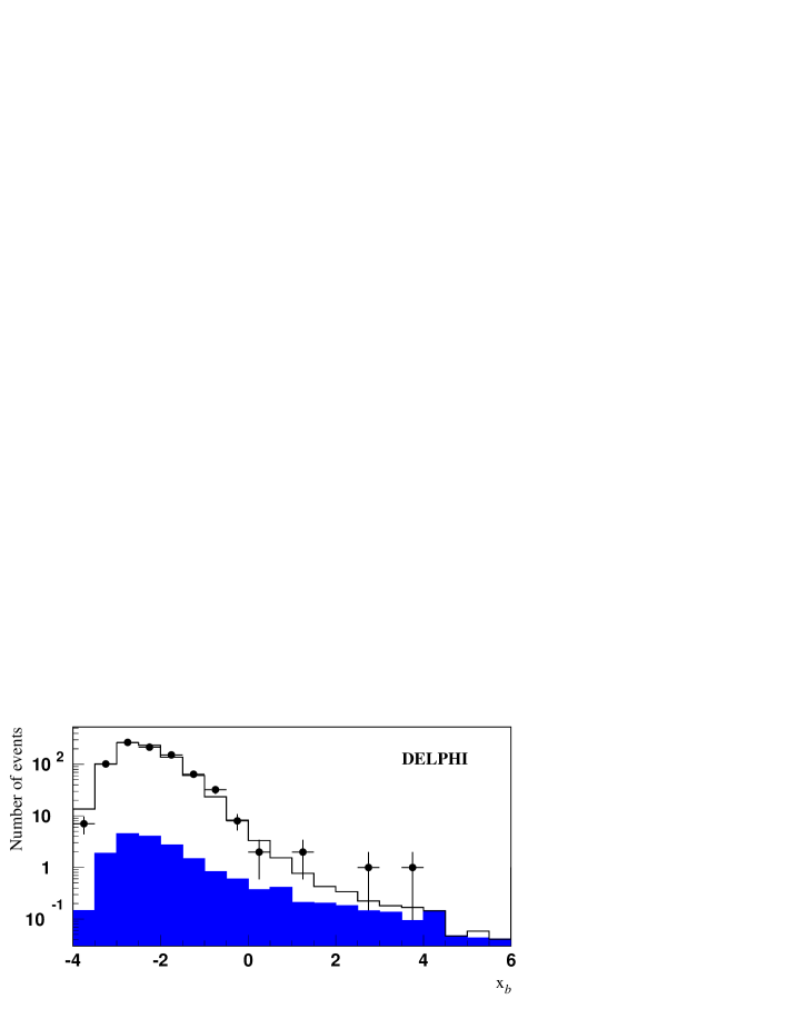
Figure 3: The b-tag obtained for semileptonic ${\mathrm{W}}^{+}{\mathrm{W}}^{-}$ decays, where the low level of b-quarks expected makes them a good sample for checking the mistagging. The solid points are the data, the open histogram the total of the simulation and the black the contribution from processes other than semileptonic ${\mathrm{W}}^{+}{\mathrm{W}}^{-}$ decays.

Also shown in Fig. 4 is the fraction of jets tagged as b-jets as a function of azimuthal angle for jets from Z particles which are in the hemisphere centred on the positron beam direction, for data taken when the TPC sector was off. A significant degradation is seen in this small region, well matched by simulation.

Figure 4: The fraction of jets tagged as b-jets as a function of azimuthal angle in the hemisphere centred on the positron beam direction, after the TPC sector located from -90^∘ to -30^∘ failed. The jets are from on peak Z events, and have $x_{\mathrm{b}}^{i}$ greater than -0.5. The points are the data, and the line shows the simulation. The opposite hemisphere is not affected.

4.4 Structure of the analysis

The analysis for each channel takes the same basic pattern. A fairly loose selection is applied which results in many candidates, which are used to calculate the overall likelihood of the signal hypothesis. The densities of signal and background processes for any measured combination of discriminant variable (channel dependent) and candidate mass are estimated using Monte Carlo simulation for the centre-of-mass energies and Higgs masses which have been discussed in sections 2 and 3. These are interpolated to give signal and background densities corresponding to the required beam energy and Higgs mass hypothesis under consideration. To simplify the analysis, the data events are treated as having the mean energy of the energy bin into which they fell, so all events in that bin are treated together.

The estimated signal and background densities at the event are used to find how much more probable the event is if the signal existed. The use of a likelihood fit to extract the results means that regions with low signal purities can be included in the selected data, and each improves the separation. Loose cuts were made on the discriminant variables, with the result that from the total search over one hundred events were expected from background processes while retaining maximal sensitivity to a SM Higgs signal. This procedure has the additional advantage that the analysis is less dependent on biases from selection cuts.

4.5 Confidence level definitions and calculations

The confidence levels are calculated using a modified frequentist technique based on the extended maximum likelihood ratio [22] which has also been adopted by the LEP Higgs working group.

The basis of the calculation is the likelihood ratio test-statistic, $\cal Q$:

$$\ln\mbox{$\cal Q$}=-S+\sum_{i}\ln\frac{s_{i}+b_{i}}{b_{i}}$$

where the $S$ is the total signal expected and $s_{i}$ and $b_{i}$ are the signal and background densities for event $i$. These densities are constructed using two-dimensional discriminant information in all channels, as in our previous publication [1]. The first variable is the reconstructed Higgs boson mass (or the sum of the reconstructed h and A masses in the ${\mathrm{h}}{\mathrm{A}}$ channels), the second one is channel-dependent, as specified in the following sections.

The observed value of $\cal Q$ is calculated using the two-dimensional Probability Density Functions (PDFs) of the variables chosen for each channel. The PDFs for $\cal Q$, which is naturally one-dimensional, are built using Monte Carlo sampling making the assumption that background processes only or that both signal and background are present, and the confidence levels $\rm CL_{\rm b}$ and $\rm CL_{\rm s+b}$ are their integrals from $-\infty$ to the observed value of $\cal Q$. Systematic uncertainties in the rates of signal or background events are taken into account in the calculation of the PDFs for $\cal Q$ by randomly varying the expected rates while generating the distribution [23], which has the effect of broadening the expected $\cal Q$ distribution and therefore making any extreme total observed likelihood value seem more probable.

$\rm CL_{\rm b}$ is the p-value for the hypothesis that only background processes are present, i.e. the probability of obtaining a result as background-like or more so than the one observed if the background hypothesis is correct. It will tend toward one if there is a signal present, and is typically 0.5 if only background is there. Similarly, the confidence level for the hypothesis that both signal and background are present, $\rm CL_{\rm s+b}$, is the probability, in this hypothesis, to obtain more background-like results than those observed. It is the p-value for the hypothesis that both signal and background events were present. The quantity $\rm CL_{\rm s}$ is defined as the ratio of these two probabilities, $\rm CL_{\rm s+b}$/$\rm CL_{\rm b}$. It is not a true confidence level, but a conservative pseudo-confidence level for the signal hypothesis. The division by $\rm CL_{\rm b}$ means that $\rm CL_{\rm s}$ is similar to $\rm CL_{\rm s+b}$ when $\rm CL_{\rm b}$ is close to one, but increases the signal confidence when a result in the background-like region is obtained. It is always larger than $\rm CL_{\rm s+b}$, such that it reflects how many times less likely the result is if the signal is present, and so gives a more conservative limit which is designed to avoid the possibility of excluding the Higgs in an experiment which has no sensitivity to it. That is to say, the use of $\rm CL_{\rm s}$ increases the signal confidence interval in the background-like region compared to $\rm CL_{\rm s+b}$. 1-$\rm CL_{\rm s}$ measures the confidence with which the signal hypothesis can be rejected and, because it is conservative, will be at least 95% for an exclusion confidence of 95%.

4.5.1 Estimation of distributions of mass and tag variable.

The Probability Density Functions (PDFs) of the mass and the channel-dependent Higgs tagging variable are required to check the consistency of the data with the background and signal processes. They were treated as having two components: the overall normalization and the shape of the distribution.

In the case of a background process PDF, the normalization was calculated from the number of simulated events of each background class passing the cuts. For the signal the measured efficiencies had also to be interpolated to estimate efficiencies at Higgs boson masses which were not simulated. In most cases this was done using one polynomial to describe the slow rise, and a second to handle the kinematic cut-off, which can be much more abrupt. For the cases where two signal masses must be allowed, a two-dimensional parameterization was used.

The shapes of the PDFs were derived using two-dimensional histograms which are taken from the simulated events. The two dimensions were the Higgs boson mass estimator and a channel-dependent Higgs tag. These distributions were smoothed using a two-dimensional kernel, which consists of a Gaussian distribution with a small component of a longer tail. The global covariance of the distribution was used to determine the relative scale factors of the two axes. The width of the kernel varied from point to point, such that the statistical error on the estimated background processes was constant at 20%. Finally multiplicative correction factors (each a one-dimensional distribution for one of the two dimensions of the PDF) were derived such that when projected onto either axis the PDF has the same distribution as would have been observed if it had been projected onto the axis first and then smoothed. This makes better use of the simulation statistics if there are features which are essentially one-dimensional, such as mass peaks.

The error parameter fixed to 20% was an important choice. It was set by dividing the background simulation into two subsamples, generating a PDF with one and using the other to test for over-training by calculating the $\rm CL_{\rm b}$ obtained from simulation of background events. This should be 0.5 if the results are not to be biased, and a value of 20% for the error gave the closest approximation to 0.5. An accurate description of the background is very important in a search for a new particle.

The simulations were made at fixed beam energies and Higgs boson masses, but in order to test a continuous range of masses and beam energies, interpolation software [24] was used to create signal PDFs at arbitrary masses and at the correct centre-of-mass energies as well as background process PDFs at the correct centre-of-mass energies. This was done by linearly interpolating the cumulative distributions. The procedure was essentially the same whether it is the beam energy or the signal mass which is being interpolated, and has been tested over ranges up to 40 ${\mathrm{GeV}}/c^{2}$ in mass. The actual shifts were up to 0.3 ${\mathrm{GeV}}$ in $\sqrt{s}$, and 5 ${\mathrm{GeV}}/c^{2}$ in mass for the Standard Model Higgs overall, but less than 0.5 ${\mathrm{GeV}}/c^{2}$ for Higgs boson masses between 113.5 and 116.5 ${\mathrm{GeV}}/c^{2}$. Comparisons of simulated and interpolated distributions for a given mass show good agreement.

5 Higgs boson searches in events with jets and electrons

The analysis used a cut based method to separate signal from background. It was very similar to that used in [1], but it has been modified to increase the sensitivity to low mass signals. The event b-tag variable was used as the second variable in the CL calculations.

The preselection required at least 8 charged particles, a total energy above 0.12$\sqrt{s}$ and at least one pair of charged particles with energies above 10 ${\mathrm{GeV}}$ (where the energy was determined from the tracking information and, when available, the calorimeter measurement) and track impact parameters below 2 mm (1 cm) in the transverse plane (along the beam direction). These tracks were required to have either an associated shower in the electromagnetic calorimeter (tight electron candidates) or point to an insensitive calorimeter region (loose electron candidates). The tight candidates had to have a total associated energy in the last three layers of the hadron calorimeter of less than 1.6 ${\mathrm{GeV}}$ and an E/p ratio above 0.3. The loose candidates had to have a normalised measured ionization energy loss in the TPC above 1.4. The total energy of other particles within 5^∘ of each candidate electron had to be less than 8 ${\mathrm{GeV}}$. The sum of the calorimetric energies of the two candidates was required to exceed 10 ${\mathrm{GeV}}$. After removing the electron candidates, the remaining particles were forced into two jets, and it was required that each of them contained at least 3 charged particles.

Bhabha events showering in the detector material were vetoed by rejecting cases where the charged multiplicity was less than or equal to 12 if a candidate electron had an energy above 70 ${\mathrm{GeV}}$ and an angle with respect to either of the beams below 25^∘ or if the acoplanarity was below 3^∘ and both electron candidates had an energy above 40 ${\mathrm{GeV}}$.

To reduce the contributions from the $\mbox{Z}\gamma^{*}$ and ${\mathrm{q}}\bar{\mathrm{q}}(\gamma)$ backgrounds, the sum of the di-electron and hadronic system unfitted masses had to be above 50 ${\mathrm{GeV}}/c^{2}$, while the missing momentum was required to be below 50 ${\mathrm{GeV}}/c$ if its direction was within 10^∘ of the beam axis.

After this preselection, each pair of electron candidates with opposite charges was subjected to further cuts. The electron identification was first tightened, allowing at most one electron candidate in the insensitive regions of the calorimeters. The two electrons were required to have energies above 20 ${\mathrm{GeV}}$ and 15 ${\mathrm{GeV}}$, respectively. Electron isolation angles with respect to the closest jet were required to be more than 20^∘ for the more isolated electron and more than 8^∘ for the other one.

There were two different mass estimators used in this analysis: a four-constraint kinematic fit imposing energy and momentum conservation, and a five-constraint kinematic fit taking into account the Breit-Wigner shape of the Z resonance [25]. The latter was used to test the compatibility of the ${\mathrm{e}}^{+}{\mathrm{e}}^{-}$ invariant mass with the Z mass and provided a better resolution in case of signal events. Events with a 5C fit probability below 10^-8 were rejected. If the 5C fitted Higgs boson mass was greater than 60 ${\mathrm{GeV}}/c^{2}$, the event was accepted as a candidate for a high mass signal. To reduce the background it was required that the sum of the 4C fitted masses of the electron pair and of the hadronic system was above 150 ${\mathrm{GeV}}/c^{2}$. If the fitted mass was less than 60 ${\mathrm{GeV}}/c^{2}$, the requirement on the sum of the masses was relaxed to 100 ${\mathrm{GeV}}/c^{2}$ to improve efficiency for low mass signals. The difference between the hadronic and the di-electron mass was required to be below 100 ${\mathrm{GeV}}/c^{2}$. The 5C fitted hadronic mass and the ${\mathrm{b}}$-tagging variable $x_{\mathrm{b}}$ were used in the two-dimensional calculation of the confidence levels.

Selection	Data	Total	${\mathrm{q}}\bar{\mathrm{q}}(\gamma)$	4 fermion	Efficiency (%)
		background
H${\mathrm{e^{+}e^{-}}}$  channel 163.3 pb-1
Preselection	936	942 $\pm$ 2	604	333	79.5
Electron identification	69	67.8 $\pm$ 0.4	17.9	49.3	67.0
Candidate selection	11	10.5 $\pm$ 0.1	0.7	9.7	59.0
H$\mu^{+}\mu^{-}$ channel 164.1 pb-1
Preselection	2678	2688 $\pm$ 6	1833	801	80.6
Muon identification	14	12.8 $\pm$ 0.2	0.2	12.6	71.5
Candidate selection	6	8.39 $\pm$ 0.14	0.04	8.35	67.0
Tau channel 163.7 pb-1
Preselection	6862	6534 $\pm$ 4	3894	2639	96.1
${\ell^{+}\ell^{-}}$${\mathrm{q}}\bar{\mathrm{q}}$	14	15.1 $\pm$ 0.12	0.5	14.6	18.4
Candidate selection	6	5.1 $\pm$ 0.07	0.1	5.0	16.3
H$\nu\bar{\nu}$ channel 157.8 pb-1(Low mass analysis)
Anti $\gamma\gamma$	13038	12890 $\pm$ 10	9669	2929	85.6
Preselection	787	786 $\pm$ 4	463	290	70.7
Candidate selection	68	67.0 $\pm$ 0.8	31.5	35.5	55.3
H$\nu\bar{\nu}$ channel 157.8 pb-1(High mass analysis)
Anti $\gamma\gamma$	13546	13361 $\pm$ 11	10023	2964	86.2
Preselection	672	621 $\pm$ 3	328	280	66.3
Candidate selection	71	72.6$\pm$ 0.9	32.1	40.5	59.0
$\mbox{H}{\mathrm{q\bar{q}}}$ channel 163.7 pb-1
Preselection	1701	1686 $\pm$ 2	473	1213	85.0
Candidate selection	31	35.5 $\pm$ 0.3	12.1	23.6	56.5

Table 2: Effect of the selection cuts for the SM channels on data, simulated background processes and simulated signal events during the first operational period. Efficiencies are given for a signal with $m_{\mathrm{H}}\,$ = 115 ${\mathrm{GeV}}/c^{2}$ at 206.5 ${\mathrm{GeV}}$. The quoted errors are statistical only. For each channel, the first line shows the integrated luminosity used; the line labelled ‘candidate selection’ shows the data selection used for calculating the confidence levels. The total background can include small contributions from sources, such as the two photon interaction process, not listed explicitly. The excess in the tau channel is discussed in sectrion 7.

Selection	Data	Total	${\mathrm{q}}\bar{\mathrm{q}}(\gamma)$	4 fermion	Efficiency (%)
		background
H${\mathrm{e^{+}e^{-}}}$channel 59.1 pb-1
Preselection	348	352 $\pm$ 1.3	226	124	78.1
Electron identification	17	23.9 $\pm$ 0.2	6.4	17.5	62.4
Candidate selection	4	3.7 $\pm$ 0.1	0.3	3.4	55.0
H$\mu^{+}\mu^{-}$channel 60.1 pb-1
Preselection	1142	1156 $\pm$ 6	788	317	81.7
Muon identification	4	4.92 $\pm$ 0.08	0.11	4.81	72.0
Candidate selection	2	3.15 $\pm$ 0.06	0.02	3.12	67.1
Tau channel 60.1 pb-1
Preselection	2636	2395 $\pm$ 4	1398	997	95.9
${\ell^{+}\ell^{-}}$${\mathrm{q}}\bar{\mathrm{q}}$	3	4.9 $\pm$ 0.2	0.3	4.6	16.2
Candidate selection	1	2.08 $\pm$ 0.12	0.1	1.9	15.1
H$\nu\bar{\nu}$ channel 57.5 pb-1(Low mass analysis)
Anti $\gamma\gamma$	4475	4539 $\pm$ 6	3388	1060	85.1
Preselection	303	288 $\pm$ 2.7	168	107	70.4
Candidate selection	22	25.0 $\pm$ 0.4	11.3	13.7	53.6
H$\nu\bar{\nu}$ channel 57.5 pb-1(High mass analysis)
Anti $\gamma\gamma$	4571	4828 $\pm$ 7	3617	1080	86.5
Preselection	234	236 $\pm$ 2.2	125	104	66.4
Candidate selection	28	28.0 $\pm$ 0.4	11.7	14.8	58.1
$\mbox{H}{\mathrm{q\bar{q}}}$ channel 60.1 pb-1
Preselection	577	619 $\pm$ 1.2	174	446	85.2
Candidate selection	9	12.2 $\pm$ 0.2	4.2	8.0	55.0

Table 3: As in Table 2, during the second operational period.

Figure 5: Efficiencies of the candidate level selection in the first data taking period, as a function of the mass of the Higgs boson and at $\sqrt{s}\,$=206.5 ${\mathrm{GeV}}$. The errors are statistical only, and the curves drawn to guide the eye. Only efficiencies higher than 5% are shown. The efficiency of the high-mass H$\nu\bar{\nu}$ analysis is only shown above a mass value of 80 ${\mathrm{GeV}}/c^{2}$.

The effect of the selections on data and simulated samples are detailed in Tables 2 and 3, while the efficiencies at the end of the analysis in the first period are shown as a function of the Higgs boson mass in Fig. 5 and for both periods in Table 10. The efficiency in the later period is typically within 2% absolute of that in the earlier.

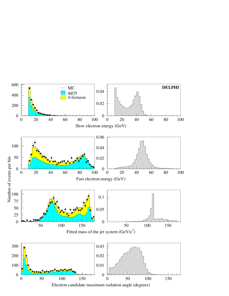
Figure 6: H${\mathrm{e^{+}e^{-}}}$ channel: distributions of four analysis variables, as described in the text, at preselection level. Data from the year 2000 (dots) are compared with SM background process expectations (left-hand side histograms). The expected distributions for a 115 ${\mathrm{GeV}}/c^{2}$ signal are shown in the right-hand side plots.

The agreement between data and simulation at the preselection level is illustrated in Fig. 6 which shows the distributions of the electron energies, the 5C fitted mass of the jet system and the isolation angle of the more isolated electron candidate. At the end of the analysis, 15 events were selected in the data for a total expected background rate of $14.2\pm 0.12(stat.)$ events coming mainly from the ${\mathrm{e}}^{+}{\mathrm{e}}^{-}$${\mathrm{q}}\bar{\mathrm{q}}$ process.

6 Higgs boson searches in events with jets and muons

The analysis used a primarily cut based method to separate signal from background. It followed the analysis published in [5, 25, 1], with slight modifications to improve the sensitivity for low Higgs boson masses. The event b-tag variable was used as the second variable in the CL calculations.

The preselection in the first (second) operational period required at least two (one) high quality track(s) of particle(s) with a transverse momentum greater than 5 ${\mathrm{GeV}}/c$. High quality tracks have impact parameters less than 100 $\mu$m in the transverse plane and less than 500 $\mu$m along the beam direction. Furthermore, there had to be at least 9 charged particles with two of them in the central part of the detector, $40^{\circ}<\theta<140^{\circ}$. The final requirement of the preselection was that there be at least two particles of opposite charges with momenta greater than 15 ${\mathrm{GeV}}/c$.

The rest of the analysis was based upon the same muon identification algorithm and discriminant variables as in [5], but the selection criteria were re-optimised. At least two charged particles were required with opposite charges and an opening angle larger than 10^∘. The muon identification algorithm [5], which yields five different levels of identification, was then applied to both particles of such pairs. The minimum level of muon identification required here corresponds to an efficiency of 88% per pair of muon candidates, with 8.8% of the pairs containing at least one pion. A jet reconstruction algorithm was then applied to the hadronic system recoiling from the muon pair, as explained in [5]. In contrast with previous analyses, no selection was applied on the number of jets in the recoiling system, nor on the number of particles in these jets, in order to increase the sensitivity to low Higgs boson masses. This leads to no significant increase of the background.

The muons were required to have momenta greater than 28 ${\mathrm{GeV}}/c$ and 21 ${\mathrm{GeV}}/c$, and their angles with respect to the closest jet axis had to be greater than 12^∘ for the more isolated muon and greater than 9^∘ for the other one.

A five-constraint kinematic (5C) fit taking into account energy and momentum conservation and the Breit-Wigner shape of the Z resonance was performed to test the compatibility of the di-muon mass with the Z mass in a window of $\pm$ 30 ${\mathrm{GeV}}/c^{2}$ around the Z pole. Events were kept only if the fit converged in this mass window. A second similar four-constraint fit (4C) was performed afterwards to take into account the possible loss of an ISR photon produced in the beam direction. The results of the 4C procedure superseded that of the 5C one if the momentum of the fitted ISR photon was greater than 10 ${\mathrm{GeV}}/c$ and if the 4C fit probability was greater than that of the 5C fit. As in the H${\mathrm{e^{+}e^{-}}}$ channel, the fitted mass of the hadronic system and the ${\mathrm{b}}$-tagging variable $x_{\mathrm{b}}$ were chosen as the discriminant variables for the two-dimensional calculation of the confidence levels.

The effect of the selections on data and simulated samples for the two periods of data taking are detailed in Tables 2 and 3. The signal efficiencies for the first period are shown as a function of Higgs boson mass in Fig. 5 and for both periods in Table 10. The rise of efficiency in the second period is due to the relaxation of the track quality cuts as described above. The agreement of simulation with data is quite good, as illustrated at preselection level in Fig. 7, which shows the multiplicity of the charged particles, the momentum of the higher-momentum particle in any preselected pair, the isolation angle of the more isolated particle in any preselected pair and the ${\mathrm{b}}$-tagging variable $x_{\mathrm{b}}$.

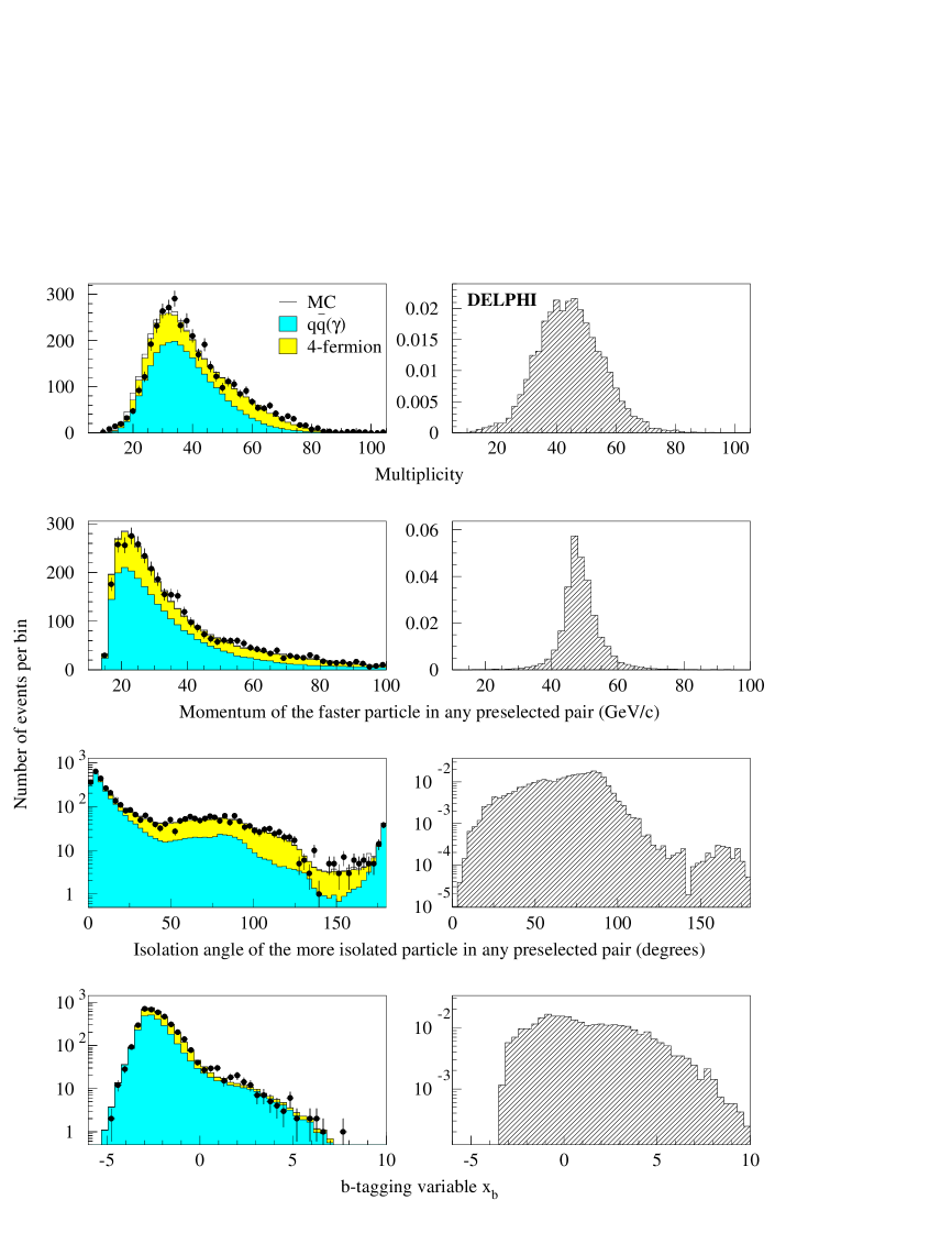
Figure 7: H$\mu^{+}\mu^{-}$ channel: distributions of four analysis variables, as described in the text, at preselection level. Data from the year 2000 (dots) are compared with SM background process expectations (left-hand side histograms). The expected distributions for a 115 ${\mathrm{GeV}}/c^{2}$ Higgs signal are shown in the right-hand side plots.

7 Higgs boson searches in events with jets and taus

The analysis used a cut based method to identify tau pairs and jet pairs, and then a likelihood variable based on kinematics and ${\mathrm{b}}$-tagging as the second variable in the CL calculations. Four channels are covered by these searches, two for the ${\mathrm{HZ}}$ channel, depending on which boson decays into $\tau^{+}\tau^{-}$, and similarly two for the ${\mathrm{h}}{\mathrm{A}}$ channel. One data set is selected, containing events from all decay channels. The analysis, almost identical to that described in [25], selected hadronic events by requiring at least ten charged particles, a total reconstructed energy greater than $0.4\mbox{$\sqrt{s}\,$}$, a reconstructed charged energy above $0.2\mbox{$\sqrt{s}\,$}$ and $\sqrt{s^{\prime}}$ greater than 120 ${\mathrm{GeV}}$.

A search for $\tau$ lepton candidates was then performed using a likelihood ratio technique. Single charged particles were preselected if they were isolated from all other charged particles by more than 10^∘, if their momentum was above 2 ${\mathrm{GeV}}/c$ and if all neutral particles in a 10^∘ cone around their direction made an invariant mass below 2 ${\mathrm{GeV}}/c^{2}$. The likelihood variable was calculated for the preselected particles using distributions of the particle momentum, isolation angle and the probability that it came from the primary vertex. Fig. 8a shows the distribution of the isolation angle of the preselected charged particle with the highest $\tau$ likelihood variable in the event for data and simulation. There is an excess of data seen at very low isolation angles. The simulation is known to underestimate the contributions from Bhabha events and the two photon interaction process in this region, which is therefore cut away.

Pairs of $\tau$ candidates were then selected requiring opposite charges, an opening angle greater than 90^∘ and a product of the $\tau$ likelihood variables above 0.45. If more than one pair was selected, only the pair with the highest product was kept. The distribution of the highest product of two $\tau$ likelihood variables in the event is given in Fig. 8b. The discrimination between the Higgs signal and the SM background processes is clearly visible. The percentage of $\tau$ pairs correctly identified was over 90% in simulated Higgs events.

Figure 8: $\tau^{+}\tau^{-}$${\mathrm{q}}\bar{\mathrm{q}}$ channel: distributions of four analysis variables at different levels of the selection, as described in the text. Data from the year 2000 (dots) are compared with SM background process expectations (left-hand side histograms). The expected distributions for a 115 ${\mathrm{GeV}}/c^{2}$ Higgs signal in the (H$\rightarrow$$\tau^{+}\tau^{-}$)(Z$\rightarrow$${\mathrm{q}}\bar{\mathrm{q}}$) channel are shown in the right-hand side plots.

Two slim jets were reconstructed with all neutral particles inside a 10^∘ cone around the directions of the $\tau$ candidates. The rest of the event was forced into two jets. The slim jets were required to be in the 20^∘$\leq~{}\theta_{\tau}~{}\leq$ 160^∘ polar angle region to reduce the ${{\mathrm{Z}e}}^{+}{{\mathrm{e}}}^{-}$ background, while the hadronic jet pair invariant mass was required to be between 20 and 110 ${\mathrm{GeV}}/c^{2}$ in order to reduce the ${\mathrm{q}}\bar{\mathrm{q}}(\gamma)$ and ${\mathrm{Z}}\gamma^{*}$ backgrounds. The jet energies and masses were then rescaled, imposing energy and momentum conservation, to give a better estimate of the masses of both jet pairs ($\tau^{+}\tau^{-}$ and ${\mathrm{q}}\bar{\mathrm{q}}$). The rescaled masses were required to be above 20 ${\mathrm{GeV}}/c^{2}$, and below $\sqrt{s}\,$ to discard unphysical solutions of the rescaling procedure. Both hadronic jets had to have rescaling factors in the range 0.4 to 1.5.

The remaining background processes were mostly genuine ${\ell^{+}\ell^{-}}$${\mathrm{q}}\bar{\mathrm{q}}$ events. In order to reject leptonic Z decays producing ${\mathrm{e}}^{+}{\mathrm{e}}^{-}$${\mathrm{q}}\bar{\mathrm{q}}$ and $\mu^{+}\mu^{-}$${\mathrm{q}}\bar{\mathrm{q}}$, the measured mass of the leptonic system was required to be between 10 and 80 ${\mathrm{GeV}}/c^{2}$ and its electromagnetic energy to be below 60 ${\mathrm{GeV}}$ (see Fig. 8c). This concluded the selection procedure. The effect of the selections on data and simulated samples is detailed in Tables 2 and 3. Efficiencies for the SM process in the first period can be found as a function of Higgs boson mass in Fig. 5 and for both periods in Table 10. The efficiencies for the MSSM channels for some selected points are given in Table 13 and in Fig. 9.

Figure 9: hA channels: efficiencies at the candidate selection level at $\sqrt{s}\,$=206.5 ${\mathrm{GeV}}$ in the first data taking period. The open symbols are for the ${\mathrm{hA}}\rightarrow\tau^{+}\tau^{-}{\mathrm{b}\bar{b}}$  analysis and the solid ones for the hA$\rightarrow$${\mathrm{b}}\bar{\mathrm{b}}$${\mathrm{b}}\bar{\mathrm{b}}$. The different shapes correspond to three different mass difference criteria for the h and A: triangles are for equal masses, squares are for the A mass fixed to 70 ${\mathrm{GeV}}/c^{2}$ and circles for $m_{A}=12$ ${\mathrm{GeV}}/c^{2}$. The errors shown are statistical only. Only efficiencies above 5% are shown; the ${\mathrm{hA}}\rightarrow\tau^{+}\tau^{-}{\mathrm{b}\bar{b}}$  channels have no points for $m_{\mathrm{A}}$ = 12 ${\mathrm{GeV}}/c^{2}$. The curves are drawn to guide the eye.

At the end of the analysis, 7 events were selected in data for a total expected background of $7.2\pm 0.1(stat.)$ events, coming mainly from the $\tau^{+}\tau^{-}$${\mathrm{q}}\bar{\mathrm{q}}$ (predominantly ZZ) and $\tau\nu$${\mathrm{q}^{\prime}}\bar{\mathrm{q}}$  (predominantly WW) processes.

The two-dimensional calculation of the confidence levels uses the reconstructed mass given by the sum of the $\tau^{+}\tau^{-}$ and ${\mathrm{q}}\bar{\mathrm{q}}$ jet pair masses after rescaling and a likelihood variable built from the distributions of the rescaling factors of the $\tau$ jets, the $\tau$ momenta and the ${\mathrm{b}}$-tagging variable, $x_{\mathrm{b}}$. The distribution of this likelihood variable at the end of the analysis is shown in Fig. 8d. Since all the $\tau^{+}\tau^{-}$${\mathrm{q}}\bar{\mathrm{q}}$ signals are covered by the same analysis, the corresponding channels cannot be considered as independent in the confidence level computation. Therefore they were combined into one global $\tau^{+}\tau^{-}$${\mathrm{q}}\bar{\mathrm{q}}$ channel: at each test point, the signal expectations (rate, two-dimensional distribution) in this channel were obtained by summing the contributions from all the original signals weighted by their expected production rates.

8 Higgs boson searches in events with missing energy and jets

The signal topology in this channel is characterised by two acollinear and acoplanar jets and a measured energy significantly less than the centre-of-mass energy, due to neutrinos coming either from the decay of a Z boson or from the ${\mathrm{W}}^{+}{\mathrm{W}}^{-}$ fusion process. In addition to the irreducible $\nu\bar{\nu}{\mathrm{q}\bar{q}}$  four-fermion events, several other background processes can lead to similar topologies; for example events due to particles from one beam only, or the ${\mathrm{q}}\bar{\mathrm{q}}\gamma(\gamma)$ process with initial state radiation photons emitted along the beam axis. The signal topology and hence the dominant background processes are somewhat different when the Higgs boson mass is very close to the kinematic threshold for HZ production compared with lower masses. DELPHI chose to use two separate analyses, one optimised for masses close to the HZ kinematic threshold and the other covering masses down to the ${\mathrm{b}}\bar{\mathrm{b}}$ threshold. These two analyses are hereafter referred to as the high mass and low mass analyses. The results are never used simultaneously: instead the sensitivity of the two searches is compared for any given signal and the more powerful analysis is selected. This comparison is done independently for each data set, with the result that for $m_{\mathrm{H}}\,$ below 99 ${\mathrm{GeV}}/c^{2}$ only the low mass analysis is used, while above 116 ${\mathrm{GeV}}/c^{2}$ all results are taken from the high mass analysis. In the region where the limit is set, two of the twelve data sets use the low mass analysis.

Both analyses followed the same procedure. First, a set of preselection criteria was applied to reject most of the single-beam, Bhabha and $\gamma\gamma$ events, and to reduce the contamination of ${\mathrm{q}}\bar{\mathrm{q}}(\gamma)$ and ${\mathrm{W}}^{+}{\mathrm{W}}^{-}$ events. For the final step of the analysis, the separation between the signal and the background channels was achieved through a multidimensional variable built with the likelihood ratio method. After a loose cut on the likelihood variable, the two-dimensional calculation of the confidence levels used the final multi-variable likelihood and the reconstructed Higgs boson mass, defined as the visible mass given by a one-constraint fit, where the recoil system is an on-shell Z boson.

A third analysis provided a cross-check of the high mass analysis. This analysis uses preselection criteria similar to the two others, but the multidimensional variable was derived using a two step discriminant analysis.

The three analyses are presented in the next sections, but they all use the following algorithms. Events were forced into two jets (the so called “two-jet configuration”) but for each event jets were also reconstructed using a distance of $y_{cut}=0.005$ (the so-called “free-jet configuration”) and general variables of each jet (such as multiplicities and momenta) were calculated in both configurations. In order to tag isolated particles from semi-leptonic decays of ${\mathrm{W}}^{+}{\mathrm{W}}^{-}$ pairs, an energy fraction was defined which was the total energy emitted at angles between 5^∘ and 25^∘ of the direction of the particle under study divided by the energy of that particle. This was calculated for the most isolated and the most energetic particles, and the smaller of these two normalised energies defined the anti-${\mathrm{W}}^{+}{\mathrm{W}}^{-}$ isolation variable, which was used in the three analyses in the determination of the final discriminant variable.

8.1 Low mass Higgs bosons with missing energy

The low mass analysis is essentially the same as that described in [1]. The preselection criteria remain unchanged.

The discriminant variable is a likelihood, constructed by multiplying the likelihoods (and neglecting correlations) from eleven discriminant variables : the angle between the missing momentum and the closest jet in the free-jet configuration, the polar angle of the more forward jet in the two-jet configuration, the polar angle of the missing momentum, the acoplanarity in the two-jet configuration, the ratio between $\sqrt{s^{\prime}}$ and the centre-of-mass energy, the missing mass of the event, the anti-${\mathrm{W}}^{+}{\mathrm{W}}^{-}$ isolation variable, the largest transverse momentum with respect to its jet axis of any charged particle in the two-jet configuration, the minimum jet charged multiplicity in the free-jet configuration, the ${\mathrm{b}}$-tagging variable $x_{\mathrm{b}}$ and the event lifetime probability $P^{+}_{\mathrm{E}}$ . The first five variables discriminate the signal from the ${\mathrm{q}}\bar{\mathrm{q}}(\gamma)$ channel and the other variables discriminate against ${\mathrm{W}}^{+}{\mathrm{W}}^{-}$ pairs. Compared to the analysis described in [1], one variable (the DURHAM distance for the transition between the two-jet and three-jet configurations) was removed because it was found to reduce sensitivity to a low mass signal.

The likelihood functions for the eleven variables were calculated for the two operational periods separately. In each case, PDFs were obtained from simulated events, using half of the available statistics in all backgrounds and signals of masses 95, 100, 105 and 110 ${\mathrm{GeV}}/c^{2}$.

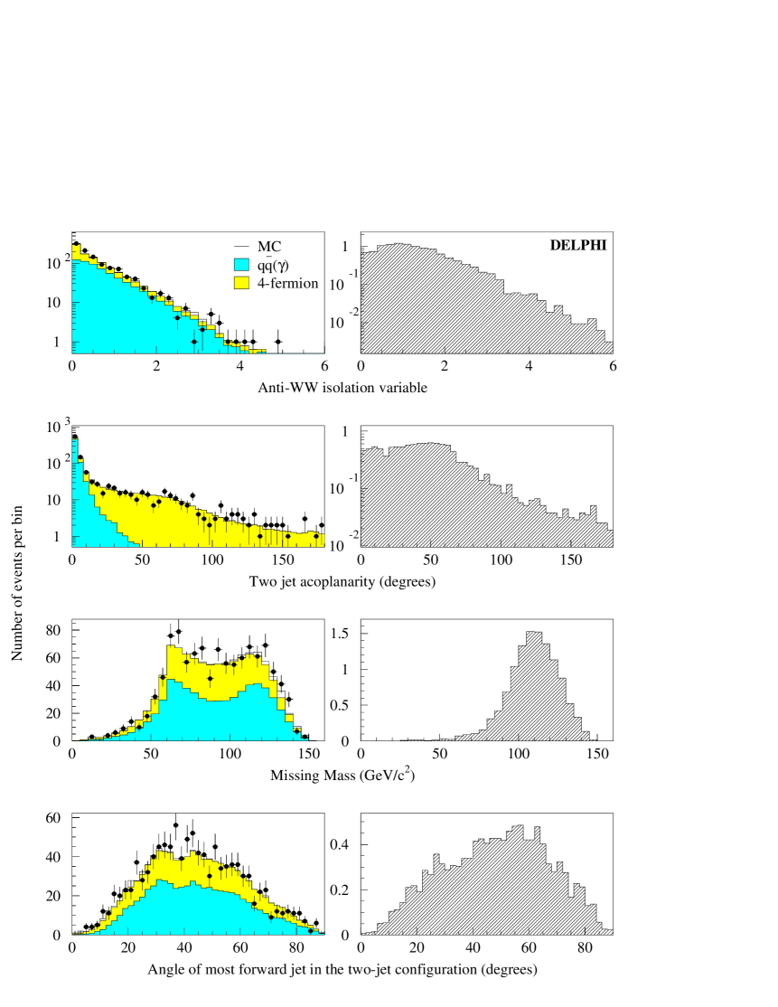
Figure 10: H$\nu\bar{\nu}$ channel low mass analysis: distributions of four analysis variables, as described in the text, at the preselection level. Data from the year 2000(dots) are compared with SM background process expectations (left-hand side histograms). The expected distributions for a 90 ${\mathrm{GeV}}/c^{2}$ signal are shown in the right-hand side plots.

The distributions of four of the input variables are shown at preselection level in Fig. 10. The comparison between the observed rate and that expected from the SM background processes in the signal-like tail of the distribution of the likelihood discriminant variable is illustrated in Fig. 11, which shows these rates as a function of the efficiency for a Higgs signal of 90 ${\mathrm{GeV}}/c^{2}$ when varying the cut on the likelihood variable. To select the candidates, a loose cut of 1,0 is applied, leaving 90 events in data for a total expected background process rate of $92.0\pm 0.9(stat.)$. The effect of the selections on data and simulated samples for the two periods of operation are detailed in Tables 2 and 3. The signal efficiencies for the first period are shown as a function of Higgs boson mass in Fig. 5 and for both periods in Table 10. Even for very low masses, this analysis has non-negligible efficiencies.

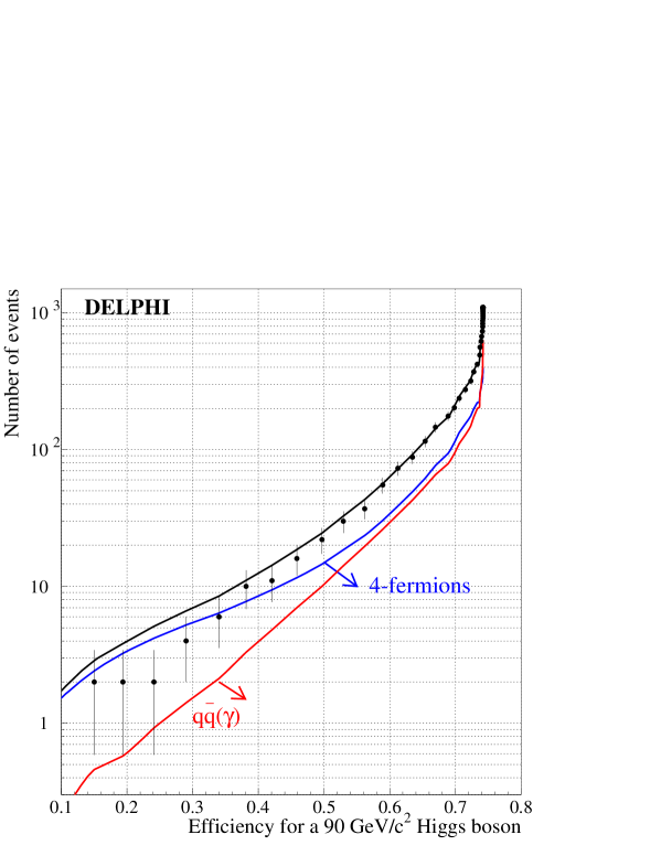
Figure 11: H$\nu\bar{\nu}$ channel, low mass analysis: the observed rate and that expected from the SM background processes as a function of the efficiency for a 90 ${\mathrm{GeV}}/c^{2}$ Higgs signal when varying the cut on the likelihood variable. The total background and different background contributions are shown separately. The dots represent the data.

8.2 High mass Higgs bosons with missing energy

The high mass analysis technique is essentially that outlined in [2]. Both the preselection criteria and the final discriminating likelihood variable were optimised to achieve the maximum reduction of the background to Higgs bosons with masses around 115 ${\mathrm{GeV}}/c^{2}$.

The general selection criteria to reject Bhabha, $\gamma\gamma$ and beam-related background events are described in [1]. Cuts were applied to reduce the ${\mathrm{q}}\bar{\mathrm{q}}(\gamma)$ channel with particular attention to all cases where fake missing energy could be created. In order to reject events coming from a radiative return to the Z with photons emitted in the beam pipe, a two-dimensional selection criterion was set in the plane of $\sqrt{s^{\prime}}$ versus the polar angle $\theta$ of the missing momentum. This selection required that $\sqrt{s^{\prime}}$ (in ${\mathrm{GeV}}$) be greater than -0.6$\times\theta$+115 ($\theta$ in degrees) for $\theta<$40^∘ (+0.6$\times\theta$+7 for $\theta>140^{\circ}$). There is no selection on $\sqrt{s^{\prime}}$ for $40^{\circ}<\theta<140^{\circ}$. To reduce the contamination of radiative return events with photons in the detector acceptance, events were rejected if the total electromagnetic energy within 30^∘ of the beam axis was greater then $0.30\sqrt{s}$. Furthermore, events were rejected if the energy deposited in the calorimeters exceeded $0.08\sqrt{s}$, $0.25\sqrt{s}$, $0.35\sqrt{s}$, $0.4\sqrt{s}$ in the small angle luminosity monitor, the forward electromagnetic calorimeter, the barrel electromagnetic calorimeter and the hadronic calorimeter, respectively. To reject events with photons crossing the small insensitive regions of the electromagnetic calorimeters, a veto based on the hermeticity counters of DELPHI similar to that of the low mass analysis [1] was also applied. To remove background events with no missing energy it was required that the effective centre-of-mass energy $\sqrt{s^{\prime}}$ was below $0.96\sqrt{s}$. Two-fermion events with jets pointing to the insensitive regions of the electromagnetic calorimeters or emitted close to the beam axis are also a potential background due to mis-measurements of the jet properties. Events were thus rejected if the jet polar angles in the two-jet configuration were within $\pm$5^∘ of 40^∘ for one jet and of 140^∘ for the other jet, unless the acoplanarity was greater than 10^∘. In addition, the acoplanarity in the two-jet configuration had to be larger than 6^∘ when the transverse momentum of the event was below 6 ${\mathrm{GeV}}/c$. The angle between either beam and the missing momentum of the event had to be greater than 10^∘. Both jets in the two-jet configuration had to be more than 12^∘  away from both the beams, or 20^∘  if the acoplanarity was less than 10^∘.

To reduce the semi-leptonic ${\mathrm{W}}^{+}{\mathrm{W}}^{-}$ background, which could fake the high mass signal topology when the leptons (especially $\tau$ particles) are hidden in the jets and thus increase the visible mass, the following selection criteria were applied. The energy of the most energetic particle in the event was required to be less than 0.20$\sqrt{s}$. At least one charged particle per jet was required for the events reconstructed in the free-jet configuration. Furthermore, when forcing the event into the two, three and free-jet configurations, there were upper limits on the transverse momentum of a charged particle with respect to its jet axis of 10, 5 and 8 ${\mathrm{GeV}}/c$ respectively. These criteria were tightened to 5, 3 and 4 ${\mathrm{GeV}}/c$ respectively when the charged particle was identified as an electron or muon using the standard criteria found in Ref. [7].

The final selection of signal-like events required that the total visible energy was less than $0.75\sqrt{s}$. All the above criteria define the preselection.

The multi-variable likelihood was constructed in the same way as in the low mass analysis and combined the following ten variables: the acoplanarity and the acollinearity in the two-jet configuration, the polar angle of the missing momentum, the ${\mathrm{b}}$-tagging variable $x_{\mathrm{b}}$, the invariant mass in the transverse plane with respect to the beam axis, the anti-${\mathrm{W}}^{+}{\mathrm{W}}^{-}$ isolation variable, the angle between the missing momentum and the closest jet in the free-jet configuration, the lowest charged multiplicity of any jet in the free-jet configuration, the largest transverse momentum with respect to its jet axis of any charged particle in the free-jet configuration, and the visible mass.

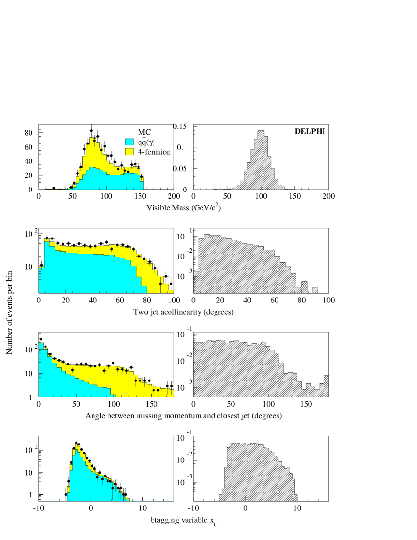
Figure 12: H$\nu\bar{\nu}$ channel, high mass analysis: distributions of four analysis variables, as described in the text, at preselection level. Data from the year 2000 (dots) are compared with SM background process expectations (left-hand side histograms). The expected distributions for a 115 ${\mathrm{GeV}}/c^{2}$ Higgs signal are shown in the right-hand side plots.

The distributions of four of the input variables are shown at preselection level in Fig. 12. The top plot of Fig. 13 shows the distribution of the likelihood discriminant variable. The comparison between the observed rates and that expected from SM background processes in the signal-like tail of this distribution is illustrated further on the bottom plot of Fig. 13, which shows these rates as a function of the efficiency to detect a Higgs boson of mass 115 ${\mathrm{GeV}}/c^{2}$ when varying the cut on the likelihood variable. To select the candidates, a minimal value of 0 is required, leaving 99 events in data for a total expected background rate of $100.6\pm 0.9(stat.)$. The effect of the selections on data and simulated samples for the two periods of operation are detailed in Tables 2 and 3. The signal efficiencies for both periods are shown as a function of the Higgs boson mass in Table 10 and for the first period in Fig. 5, where the efficiency in the low mass analysis can also be seen. The high mass analysis takes over from the low mass analysis at around 105 ${\mathrm{GeV}}/c^{2}$ and when the expected performances are calculated it brings a gain equivalent to at least 50% more luminosity for signal masses above 110 ${\mathrm{GeV}}/c^{2}$.

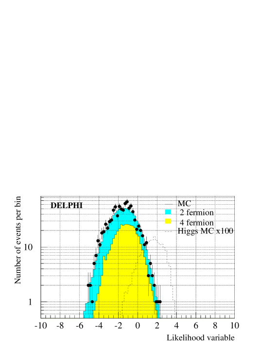
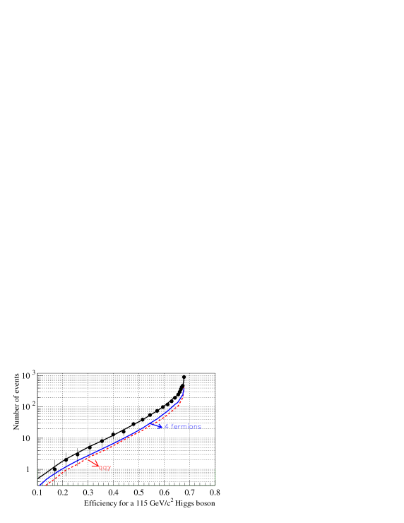
Figure 13: H$\nu\bar{\nu}$ channel, high mass analysis: Top: distributions of the likelihood variable for the expected SM background processes (full histograms), all data from the year 2000 (dots) and the expected Higgs signal at 115 ${\mathrm{GeV}}/c^{2}$ (dashed histogram, normalised to 100 times the expected rate). Bottom: The observed rate and that expected from the SM background processes at $\sqrt{s}$ = 206.5 ${\mathrm{GeV}}$ as a function of the efficiency for a 115 ${\mathrm{GeV}}/c^{2}$ Higgs signal when varying the cut on the likelihood variable. The different background contributions are shown separately. The dots represent the data.

8.3 Missing energy using Iterative Discriminant Analysis (IDA)

A second analysis optimised for high masses was made as a cross-check. This analysis used the iterative discriminant analysis (IDA) [27] method, which is a modification of Fisher’s discriminant analysis [28]. The IDA method introduces two elements, a non-linear discriminant function (whereas the Fisher function is linear) and an iterative procedure, to enhance the separation of signal events from background.

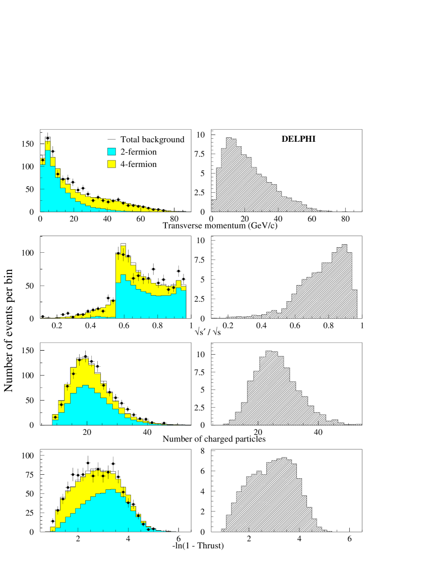
Figure 14: H$\nu\bar{\nu}$ channel, IDA analysis: distributions of four analysis variables, as described in the text, at the level of the common preselection for the IDA analysis and low mass analysis. Data (dots) are compared with SM background expectations (left-hand side histograms). The expected distributions for a 115 ${\mathrm{GeV}}/c^{2}$ Higgs signal are shown in the right-hand side plots.

The same set of preselection criteria as in the low mass analysis was applied to remove the bulk of the background events, before the IDA training. Ten variables were used to train the IDA: the ratio of visible energy to centre-of-mass energy, the energy around the most isolated particle in a double cone whose inner and outer opening angles are normally 5^∘ to 25^∘ (but do depend upon energy), the ${\mathrm{b}}$-tagging variable $x_{\mathrm{b}}$, the thrust in the rest frame of the visible system, the acoplanarity when forced to two jets scaled by the sine of the minimum angle between a jet and the beam axis, the transverse momentum, the anti-${\mathrm{W}}^{+}{\mathrm{W}}^{-}$ isolation variable as explained in section 8, $\sqrt{s^{\prime}}/\sqrt{s}$, the ${\mathrm{b}}$-tagging variable in the three-jet configuration, and the number of charged particles. Fig. 14 shows the distributions of four of the IDA variables at preselection level.

As a next step, the event samples were reduced further by imposing cuts in the tails of the signal distributions of the variables used to train the IDA. For each variable in the combined 105 to 116 ${\mathrm{GeV}}/c^{2}$ Higgs signal sample, the cuts removed about 0.5% of the events in both the upper and lower tails or about 1% if only one tail was cut on.

The IDA consisted of two steps (iterations), keeping 85% of the signal in the first iteration. The training samples were simulated signal events with Higgs boson masses between 105 and 116 ${\mathrm{GeV}}/c^{2}$. Half of the available statistics, for both signal and background samples, were used for the IDA training. The remaining events were used to derive numbers for the background event rejection and signal efficiencies, thus avoiding a statistical bias in these estimates.

Selection	Data	Total	${\mathrm{q}}\bar{\mathrm{q}}(\gamma)$	4 fermion	Efficiency (%)
		background
Missing energy IDA analysis, first period, 157.8 pb-1
Anti $\gamma\gamma$	13038	12890$\pm$ 10	9669	2929	85.6
Preselection	787	786 $\pm$ 4	463	290	70.7
eff(DA2)$=85\%$	21	16.6 $\pm$ 0.6	7.9	8.6	47.8
Missing energy IDA analysis, second period, 57.5 pb-1
Anti $\gamma\gamma$	4475	4539 $\pm$ 6	3388	1060	85.1
Preselection	303	288 $\pm$ 3	168	107	70.4
eff(DA2)$=85\%$	9	6.76 $\pm$ 0.32	3.44	3.31	47.9

Table 4: H$\nu\bar{\nu}$ channel, IDA analysis: effect of the selections on data and on simulated background and signal events. Efficiencies are given for a signal with $m_{\mathrm{H}}\,$ = 115 ${\mathrm{GeV}}/c^{2}$, $\sqrt{s}\,$=206.5 ${\mathrm{GeV}}$. The quoted errors are statistical only. For each period the first line shows the integrated luminosity used; the line labelled ‘eff(DA2)$=85\%$’ shows the results when a cut on the IDA value is applied such that the efficiency for selecting a signal is 85%; the cut value is different in the two periods.

Table 4 shows the effect of the selections on data and simulated samples.

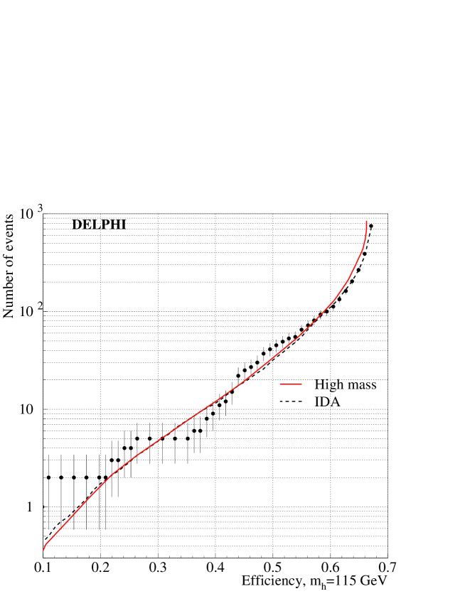
Figure 15: H$\nu\bar{\nu}$ channel, IDA analysis: the observed rate and that expected from the SM background processes as a function of the efficiency for a 115 ${\mathrm{GeV}}/c^{2}$ Higgs signal when varying the cut on the IDA variable. The solid curve, from the high mass analysis, is included so that the very similar performance of the two analyses can be seen. The dots represent the data.

Fig. 15 shows the observed rate and that expected from SM background processes as a function of the efficiency for a Higgs signal of 115 ${\mathrm{GeV}}/c^{2}$.

The two high-mass analyses have different approaches, both in the methods applied to extract the discriminant information and in the treatment of the tails. The sensitivities and the results are very similar for the two analyses, as can be seen in Figs. 13 and 15.

9 Higgs boson searches in hadronic events

The analyses in the HZ and hA channels start from an inclusive preselection, after which all selection was performed by a Neural Network which removes some of the more distinct backgrounds. The output of the Neural Network was then used as the second variable in the CL calculations. The four-jet preselection, which eliminates $\gamma\gamma$ events and reduces the contributions from the ${\mathrm{q}}\bar{\mathrm{q}}(\gamma)$ and $\mbox{Z}\gamma^{*}$ processes, was not changed since the previous analysis. The reader is referred to [5, 25] for the exact description of the cuts, while only the important features are briefly mentioned here. After a selection of multi-hadron events excluding those with an energetic photon in the calorimeters or lost in the beam pipe, topological criteria were applied to select multi-jet events. All selected events were then forced into a four-jet topology and a minimal multiplicity and mass (1.5 ${\mathrm{GeV}}/c^{2}$) was required for each jet. After the preselection, different analysis procedures were applied in the ${\mathrm{HZ}}$ and ${\mathrm{h}}{\mathrm{A}}$ channels.

9.1 The HZ four-jet channel

Two analyses were applied to the whole range of masses, and the results from the more powerful one were used. One corresponds precisely to the account published in Ref. [1], and is not described in this paper; the other has been optimised for high Higgs masses. The same automatic procedure as in the neutrino channel was applied to select only the analysis with the better performance at each test point. The range of masses where the switches from the low mass to the high mass analyses occur lay between 99 and 110 ${\mathrm{GeV}}/c^{2}$ (with the majority of the 12 data sets changing at 105 ${\mathrm{GeV}}/c^{2}$). The rest of this section describes the high-mass optimised analysis.

The final discriminant variable used in the four-jet channel was the output of an artificial neural network (ANN) which combined thirteen variables. This is the same as was used in [2] without retraining. The first of the variables was the global ${\mathrm{b}}$-tagging variable $x_{\mathrm{b}}$ of the event. The next four variables tested the compatibility of the event with the hypotheses of ${\mathrm{W}}^{+}{\mathrm{W}}^{-}$ and ${\mathrm{ZZ}}$ production giving either 4 or 5 jets. Constrained fits were used to derive the probability density function measuring the compatibility of the event kinematics with the production of two objects of hypothetical masses. This yielded a two-dimensional probability, the ideogram probability [29]. To estimate compatibility with the ${\mathrm{ZZ}}$ and ${\mathrm{W}}^{+}{\mathrm{W}}^{-}$ processes, the integral over all boson masses of the ideogram probability times the probability of obtaining that pair of masses from the process in question was calculated.

The last eight input variables, intended to reduce the ${\mathrm{q}}\bar{\mathrm{q}}(\gamma)$ contamination, were the sum of the second and fourth Fox-Wolfram moments, the product of the minimum jet energy and the minimum opening angle between any two jets, the maximum and minimum jet momenta, the sum of the multiplicities of the two jets with lowest multiplicity, the sum of the masses of the two jets with lowest masses, the minimum jet pair mass and the minimum sum of the cosines of the opening angles of the two jet pairs when considering all possible pairings of the jets. The neural network was trained on independent samples, using signal masses close to the kinematic limit.

The choice of the Higgs jet pair made use of both the kinematic 5C-fit probabilities (imposing four-momentum conservation and assigning the Z mass to one pair of jets) and the ${\mathrm{b}}$-tagging information in the event [5]. The likelihood pairing function,

$${\cal P}_{b}^{j_{1}}\cdot{\cal P}_{b}^{j_{2}}\cdot((1-R_{b}-R_{c})\cdot{\cal P}_{q}^{j_{3}}\cdot{\cal P}_{q}^{j_{4}}+R_{b}\cdot{\cal P}_{b}^{j_{3}}\cdot{\cal P}_{b}^{j_{4}}+R_{c}\cdot{\cal P}_{c}^{j_{3}}\cdot{\cal P}_{c}^{j_{4}})\cdot P_{j_{3},j_{4}}^{5C}$$

was calculated for each of the six possibilities to combine the jets $j_{1}$, $j_{2}$, $j_{3}$ and $j_{4}$ and assign the jet pairs to a H or Z hypothesis. ${\cal P}_{b}^{j_{i}},{\cal P}_{c}^{j_{i}},{\cal P}_{q}^{j_{i}}$ are the probability densities of getting the observed ${\mathrm{b}}$-tagging value for the jet $j_{i}$ when originating from a $b$, $c$ or light quark, estimated from simulation. $R_{b}$ and $R_{c}$ are the hadronic branching fractions of the Z into $b$ or $c$ quarks [30], and $P_{j_{3},j_{4}}^{5C}$ is the probability of the kinematic 5C-fit with the jets $j_{3}$ and $j_{4}$ assigned to the Z. The pairing that maximised this function was selected and the reconstructed Higgs boson mass was the result of the 5C-fit for that pairing. The proportion of right matchings for the Higgs jet pair, estimated in simulated signal events with 115 ${\mathrm{GeV}}/c^{2}$ mass, was around 53% at preselection level, increasing to 73% after a cut on ANN of 0.81, as used later for figure 21. This technique is better than using just the probability of the kinematic 5C-fit, both for ${\mathrm{HZ}}$ and ${\mathrm{ZZ}}$ events.

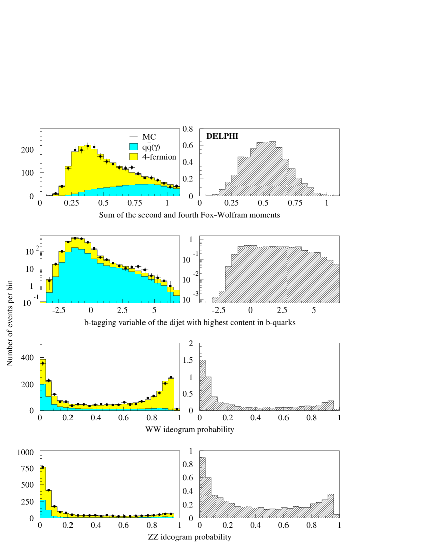
Figure 16: $\mbox{H}{\mathrm{q\bar{q}}}$ channel: distributions of four analysis variables, as described in the text, at preselection level. Data from the year 2000 (dots) are compared with SM background process expectations (left-hand side histograms). The expected distributions for a 115 ${\mathrm{GeV}}/c^{2}$ Higgs signal are shown in the right-hand side histogram.

The agreement between data and background process simulations after the four-jet preselection is illustrated in Fig. 16, which shows the distributions of the sum of the second and fourth Fox-Wolfram moments as an example of the kinematic variables, the global ${\mathrm{b}}$-tagging variable, and the WW and ZZ ideogram probabilities for the configuration with 4 jets. Fig. 17 shows the performance of the final discriminating variable in terms of the background rate as a function of the efficiency for a 115 ${\mathrm{GeV}}/c^{2}$ Higgs signal, and the agreement between simulation and data. The effect of the selections on data and simulated samples for the two periods of data taking are detailed in Tables 2 and 3. The signal efficiencies for the first period are shown as a function of the Higgs boson mass in Fig. 5 and for both periods in Table 10. The data are also analysed by the low mass analysis, which selected 180 candidates for the confidence level calculation while 173 were expected from SM background processes.

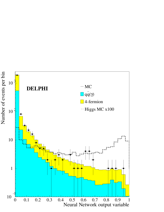
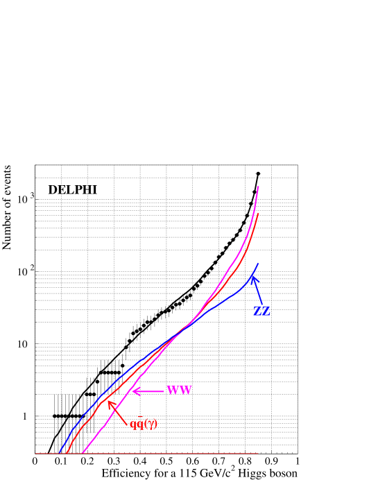
Figure 17: $\mbox{H}{\mathrm{q\bar{q}}}$ channel: Top: the distribution of the neutral network variable used to select Higgs candidates in the 2000 data. The signal expectation is shown for a 115 ${\mathrm{GeV}}/c^{2}$ Higgs, normalised to 100 times the expected rate. The dots represent the data. Bottom: curve of the expected SM background rate in the 2000 data as a function of the efficiency for a 115 ${\mathrm{GeV}}/c^{2}$ Higgs signal when varying the cut on the neural network variable. The different background contributions are shown separately. The dots represent the data.

The final CL calculations were made in the plane of the ANN value versus the Higgs boson mass estimator, using only events where the ANN was greater than 0.2. This gives 47.7$\pm$0.3(stat.) events expected from background processes, whilst 40 are observed.

9.2 The hA four-b channel

This channel benefited most from the data reprocessing and improved ${\mathrm{b}}$-tagging. The analyses include not only data from the year 2000, but also the reprocessed 1999 data. After the common four-jet preselection, events were preselected further, requiring a visible energy greater than 120 $\times\sqrt{s}/189$ ${\mathrm{GeV}}$, $\sqrt{s^{\prime}}$ greater than 150 $\times\sqrt{s}/189$ ${\mathrm{GeV}}$, a missing momentum component along the beam direction lower than 30 ${\mathrm{GeV}}/c$ and at least two charged particles per jet. A four-constraint kinematic fit requiring energy and momentum conservation was then applied, and the two jet-pair masses were calculated for each of the three different jet pairings. As the possible production of MSSM Higgs bosons through the ${\mathrm{h}}{\mathrm{A}}$ mode dominates at large $\tan\beta$, where the two bosons are almost degenerate in mass, the pairing defining the Higgs boson candidates was chosen as that which minimizes the mass difference between the two jet pairs and the reconstructed Higgs boson masses were taken from the 4C-fit for that pairing. The final discrimination between background and signal events was then based on a multidimensional variable which combined the following twelve variables as the output of an artificial neural network: the event thrust, the sum of the second and fourth Fox-Wolfram moments, the product of the minimum jet energy and the minimum opening angle between any two jets, the minimal $y_{cut}$ values for which the event is clustered into 4 jets ($y_{34}$) and into 5 jets ($y_{45}$), the maximum and minimum jet momenta, the sum of the multiplicities of the two jets with lowest multiplicity, the minimum jet pair mass, the production angle of the Higgs boson candidates, the sum of the four jet ${\mathrm{b}}$-tagging variables and the minimum jet pair ${\mathrm{b}}$-tagging variable. The neural network was trained using signal masses between 80 and 95 ${\mathrm{GeV}}/c^{2}$, and about 10% of the simulated background events, and this one training applied to all data sets.

Selection	Data	Total	${\mathrm{q}}\bar{\mathrm{q}}(\gamma)$	4 fermion	Efficiency (%)
		background
hA four-jet channel 228 pb-1 1999
Tight preselection	2224	2211.4$\pm$ 2.5	650.0	1561.4	91.6
Candidate selection	217	191.6 $\pm$ 0.8	81.4	110.2	89.0
hA four-jet channel 163.7 pb-1 2000 1st period
Tight preselection	1459	1500.2$\pm$ 2.1	406.9	1093.3	91.2
Candidate selection	127	129.3 $\pm$ 0.7	50.6	78.5	89.4
hA four-jet channel 60.1 pb-1 2000 2nd period
Tight preselection	495	547.2$\pm$ 1.1	148.1	399.1	90.8
Candidate selection	48	45.2 $\pm$ 0.3	17.4	27.8	88.2

Table 5: ${\mathrm{h}}{\mathrm{A}}$ hadronic channel: effect of the selections on data and simulated background events. Efficiencies are given for a signal with $m_{\mathrm{A}}$= $m_{\mathrm{h}}$= 90 ${\mathrm{GeV}}/c^{2}$. The quoted errors are statistical only. For each case, the first line shows the integrated luminosity used; the line labelled ‘candidate selection’ shows the events used for calculating the confidence levels.

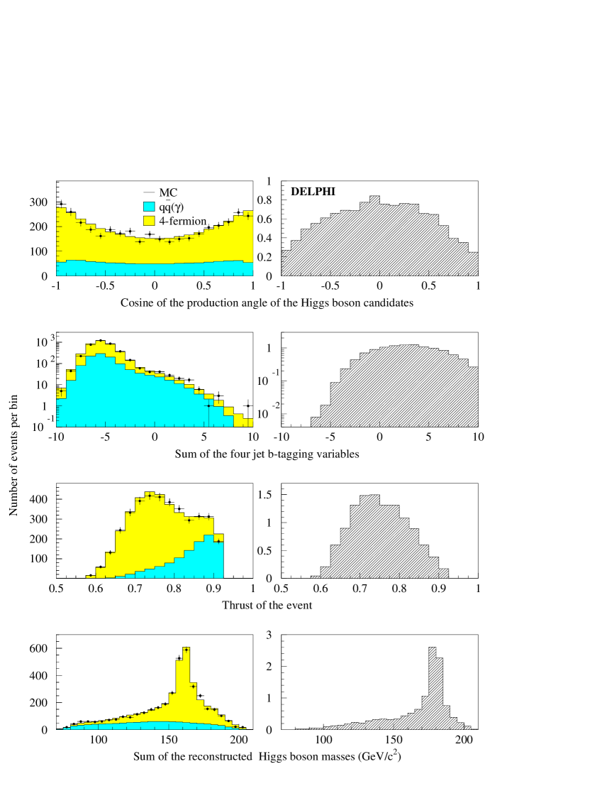
Figure 18: hA hadronic channel: distributions of four analysis variables, as described in the text, at preselection level. Data from the years 1999 to 2000 (dots) are compared with SM background process expectations (left-hand side histograms). The expected distributions for a $m_{\mathrm{A}}$= $m_{\mathrm{h}}$= 90 ${\mathrm{GeV}}/c^{2}$ signal are shown in the right-hand side plots.

The agreement between data and background channel simulations after the preselection is illustrated in Fig. 18, which shows the distributions of three input variables and of the sum of the reconstructed Higgs boson masses. Fig. 19 shows the distribution of the final discriminant variable and, as an example, the total expected background rate and the data from 1999 and 2000 as a function of the efficiency for a signal with $m_{\mathrm{A}}$= $m_{\mathrm{h}}$= 90 ${\mathrm{GeV}}/c^{2}$, when varying the cut on the discriminant variable. As a final selection, a minimal value of 0.1 is required, leading to 392 events in data, with $366.2\pm 1.1(stat.)$ expected from background processes. The effect of the selections on data and simulated samples are detailed in Table 5 while representative efficiencies at the end of the analysis are reported as a function of Higgs boson masses in Tables 11 and 13 and in Fig. 9.

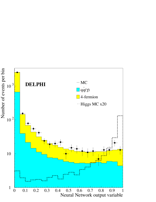
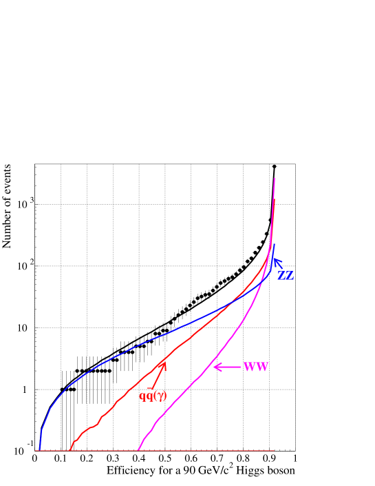
Figure 19: hA hadronic channel: Top: distributions of the ANN variable for the expected SM background processes (full histograms), the data from the years 1999 and 2000 (dots) and the expected $m_{\mathrm{A}}$= $m_{\mathrm{h}}$= 90 ${\mathrm{GeV}}/c^{2}$ Higgs signal (dashed histogram, normalised to 20 times the expected rate). Bottom: curve of the expected SM background rate for all data from 1999 and 2000 as a function of the efficiency for the same signal when varying the cut on the ANN variable. The different background contributions are shown separately. The dots show the data.

The two-dimensional calculation of the confidence levels uses the ANN variable and the sum of the reconstructed Higgs boson masses.

9.3 Additional MSSM results

In the purely hadronic final state, which is the dominant topology in the MSSM, additional signals were considered.

In a small region of the parameter space where the ${\mathrm{h}}{\mathrm{Z}}$ production process is dominant, the decay ${\mathrm{h}}\rightarrow{\mathrm{AA}}$ opens. As the low mass $\mbox{h}{\mathrm{q\bar{q}}}$ analysis proved to perform reasonably on that signal, no dedicated procedure was set up and that analysis was applied as such on the two simulated (${\mathrm{h}}\rightarrow{\mathrm{AA}}$)(${\mathrm{Z}}\rightarrow$ ${\mathrm{q}}\bar{\mathrm{q}}$) channels. The corresponding efficiencies are shown in Table 12 at $\sqrt{s}\,$=206.5 ${\mathrm{GeV}}$ for both data-taking periods. The efficiencies and PDFs obtained for the (${\mathrm{h}}\rightarrow{\mathrm{AA}}\rightarrow{\mathrm{c\overline{c}c\overline{c}}}$) (${\mathrm{Z}}\rightarrow$ ${\mathrm{q}}\bar{\mathrm{q}}$) channel were conservatively applied to the two channels where one A boson decays into b’s while the other decays into c’s.

The two four-jet final states expected in the MSSM have common features. As a consequence, the two analyses developed specifically for each of them perform rather well on the other signal. As an example, the efficiencies of the low mass $\mbox{h}{\mathrm{q\bar{q}}}$ analysis applied on the four-b signal and that of the ${\mathrm{h}}{\mathrm{A}}$ four-b analysis applied on the $\mbox{h}{\mathrm{q\bar{q}}}$ signal are given in Tables 14 and 15 at 199.6 ${\mathrm{GeV}}$  and at 206.5 ${\mathrm{GeV}}$ for both data-taking periods. Thus, when combining the results in the ${\mathrm{h}}{\mathrm{Z}}$ and ${\mathrm{h}}{\mathrm{A}}$ channels to derive confidence levels in the MSSM, both selected signals are included in the results of these two analyses at all energies above 191.6 GeV. This leads to a gain in sensitivity of around 1 ${\mathrm{GeV}}/c^{2}$ on the masses of MSSM Higgs bosons in regions of the parameter space where both the ${\mathrm{h}}{\mathrm{Z}}$ and ${\mathrm{h}}{\mathrm{A}}$ production processes contribute.

10 Systematic errors

The systematic errors for each channel are discussed below.

10.1 Systematic errors in the H${\mathrm{e^{+}e^{-}}}$  search

The systematic uncertainties on background rates and signal efficiency estimates are mainly due to the imperfect simulation of the detector response and were estimated as described in [5]: each cut in turn was adjusted until the fraction of events accepted in simulation matched that found in data. The corresponding changes in background and signal rates were summed in quadrature.

The relative error on the efficiencies is typically $\pm 2\%$ while that on the background rate estimates is $\pm 5\%$.

10.2 Systematic errors in the H$\mu^{+}\mu^{-}$ search

The imperfect simulation of the detector response leads to systematic errors in background process rate and signal efficiency evaluation. As explained in [5], each of the momentum and angular cuts was varied in a range given by the difference between the mean values of the simulated and real data distributions of the corresponding variable at preselection level. This method cannot be used for the muon pair identification tag, which is a discrete variable. To estimate the effect of possible differences in muon pair tagging between the data and the simulated samples, each muon candidate in the simulated samples was allowed to migrate randomly from its original level of identification to one of the two neighbouring ones, with a probability of 1.5%, with migrations to non-physical levels ignored. This probability corresponds to the difference observed in muon identification results between real data and simulation. For the relative error on the expected number of background events we also include a 2% uncertainty on the ${\mathrm{ZZ}}$ cross-section, so the total systematic error is estimated to be $\pm$2.8% on the background. For the efficiencies, an overall relative systematic uncertainty of $\pm 1\%$ can be quoted, independent of $m_{\mathrm{H}}\,$.

10.3 Systematic errors in the $\tau^{+}\tau^{-}{\mathrm{q}\bar{q}}$ search

Systematic uncertainties from the imperfect modelling of the detector response were estimated by moving each selection cut according to the resolution in the corresponding variable. The main contributions arise from the cuts on the $\tau^{+}\tau^{-}$ invariant mass and electromagnetic energy. The total relative systematic uncertainties amount to $\pm$6% on signal efficiencies and $\pm$11% on the background process estimates.

10.4 Systematic errors in the H$\nu\bar{\nu}$  search

Systematic uncertainties in the low mass analysis due to the imperfect modelling of the detector response were derived by rescaling, bin by bin, the contents of each PDF from simulation to those in data, restricting to bins that contained at least one percent of the total statistics. The analysis was then repeated with the rescaled PDF for each variable in turn and the largest difference with respect to the initial result was taken as systematics. These systematics amount to $2\%$ for the efficiencies and to $4\%$ for the background in the first data taking period and come from the PDF of the acoplanarity distribution. These numbers become $3\%$ and $9\%$ for the second data taking period. Systematic uncertainties due to the use of non-independent samples in the definition of the likelihood PDFs and in the final result amount to $\pm 2\%$ for the efficiencies and to $\pm 1\%$ for the background processes in the first operational period. These numbers become $\pm 3\%$ and $\pm 4\%$ for the second operational period. Thus, the overall uncertainties amount to $\pm 2.8\%$ ($\pm 4.1\%$) for the signal efficiencies and $\pm 4.1\%$ ($\pm 9.8\%$) for the background channels, for the first (second) period of data taking.

The same method was used to derive the systematic uncertainties in the high mass analysis. This was done separately for the two operational periods. Systematic uncertainties due to the use of non-independent samples in the definition of the likelihood PDFs and in the final result amount to $<\pm 1\%$ for both the signal efficiencies and the background for the two operational periods. These uncertainties are well below the statistical errors. Systematic uncertainties due to the imperfect modelling of the detector response (coming from the PDF of the visible mass distribution) amount to $\pm 1\%$ for the efficiencies and to $\pm 7\%$ for the background processes in the first operational period. These numbers become $\pm 2\%$ and $\pm 7\%$ for the second operational period.

10.5 Systematic errors in the four-jet searches

In the ${\mathrm{H}}{\mathrm{Z}}$ search the systematic uncertainties from the imperfect modelling of the detector response were estimated by repeating the selection procedure on the distribution of the neural network variable obtained by smearing, in turn, each of the distributions of the thirteen input variables according to the resolution in the variable. This leads to relative uncertainties of $\pm$5% related to b-tagging. Uncertainties in the anti-QCD variables are $\pm$2% in the background process estimations and $\pm$1% in the signal efficiencies. Systematic uncertainties related to the ideogram probabilities are $\pm$3% for the background and $\pm$2% for the efficiencies. This results in overall relative uncertainties of $\pm 6.2\%$ in the background rates and $\pm 5.5\%$ in efficiency estimates for each period.

Systematic uncertainties in the ${\mathrm{h}}{\mathrm{A}}$ search due to the use of non-independent samples in the training of the ANN and in the final result derivation were estimated at the level of $\pm 1.0\%$ relative, by repeating the whole procedure with two independent samples of smaller size. Systematic uncertainties due to the imperfect modelling of the detector response were derived as above. The uncertainty related to ${\mathrm{b}}$-tagging amounts to $\pm 10\%$ on background and $\pm 1.2\%$ on signal, while that related to shape variables is $\pm 5.0\%$ in the background rate and $\pm 1.2\%$ in signal efficiency estimates. Combining all these results in overall relative uncertainties of $\pm 11.2\%$ and $\pm 1.7\%$ on background processes and signal efficiency.

10.6 Summary of systematic errors

${\mathrm{H}}{\mathrm{Z}}$ selection	period	background	signal
H${\mathrm{e^{+}e^{-}}}$ channel	both	$\pm$5%	$\pm$2%
H$\mu^{+}\mu^{-}$ channel	both	$\pm$2.8%	$\pm$1%
Tau channel	both	$\pm$11%	$\pm$6%
H$\nu\bar{\nu}$  (low mass )	first	$\pm$4.1%	$\pm$2.8%
H$\nu\bar{\nu}$  (low mass )	second	$\pm$9.8%	$\pm$4.1%
H$\nu\bar{\nu}$  (high mass)	first	$\pm$7%	$\pm$1%
H$\nu\bar{\nu}$  (high mass)	second	$\pm$7%	$\pm$2%
$\mbox{H}{\mathrm{q\bar{q}}}$ channel	both	$\pm$ 6.2%	$\pm$5.5%
${\mathrm{h}}{\mathrm{A}}$ selection	period	background	signal
Four-jet channel	both	$\pm$11.2%	$\pm$1.7%

Table 6: The systematic error estimates for the individual channels. The missing energy channels are somewhat more sensitive to the condition of the detector, and result in the larger errors during the second period.

The error estimates obtained in each channel are shown in Table 6. In principle there might be small correlations between the errors in the different channels, from for example the cross-section of the ${\mathrm{ZZ}}$ process and the b-tagging procedure. However, both these enter in significantly different ways in the different channels, and the correlated component is therefore rather small, and has been neglected.

11 Results

The results of the searches presented in the previous sections are used to calculate the consistency of the data with signal and background hypotheses, and derive confidence levels as a function of the masses of the neutral Higgs bosons in the SM and MSSM.

11.1 Reconstructed mass spectra

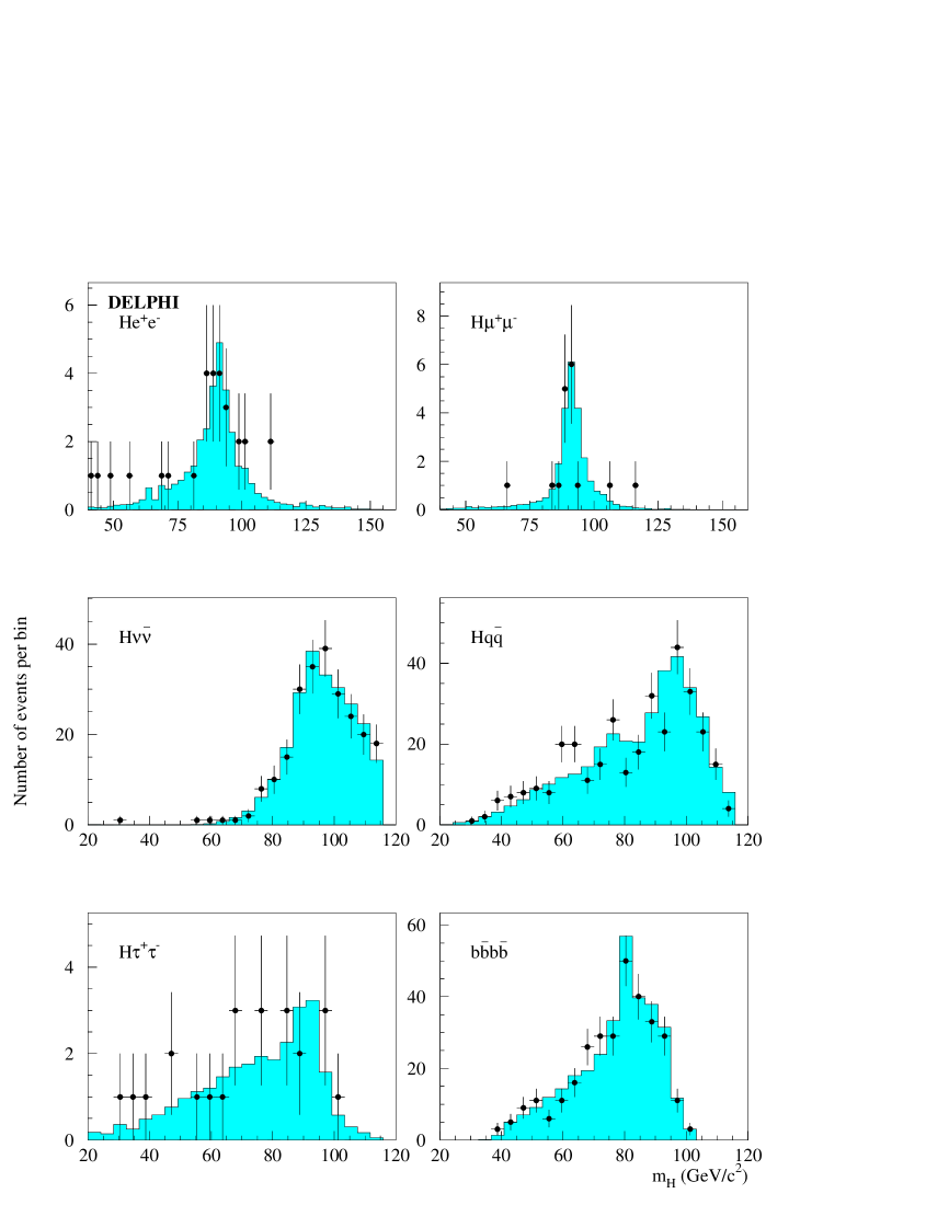
Figure 20: Distributions of the reconstructed Higgs boson mass(es) in each channel when all the data from 183 to 209 ${\mathrm{GeV}}$ are combined at the candidate selection level. This plot contains almost all the LEP2 data set used for the extraction of the final limits. Data (dots) are compared with SM background expectations (full histograms).

The distributions of the reconstructed Higgs boson mass(es) at the level of the selected candidates are presented in Fig. 20. These plots include our previous LEP2 results above 183 ${\mathrm{GeV}}/c^{2}$. The data are consistent with the simulated background events.

The results for only the year 2000 SM analysis are shown in Fig. 21. For this figure there is an extra selection: a cut on the second discriminant variable was applied such that a signal might be more apparent. This cut is fixed for all channels so that, for events with mass greater than 110 ${\mathrm{GeV}}/c^{2}$ in data taken at 206.5 ${\mathrm{GeV}}$, the signal to background ratio should be 0.75. The selections required a minimal ${\mathrm{b}}$-tagging value of 0.49 in the H${\mathrm{e^{+}e^{-}}}$ and -2.5 in the H$\mu^{+}\mu^{-}$ channels, minimal likelihood values of 0.58, 2.22 in the $\tau^{+}\tau^{-}{\mathrm{q}\bar{q}}$  and H$\nu\bar{\nu}$ channels, respectively, and a minimal neural network output of 0.81 in the $\mbox{H}{\mathrm{q\bar{q}}}$ channel. The corresponding observed and expected rates in each period are given in Table 7, which can be compared with Tables 2 and 3.

Channel	Data	Total	${\mathrm{q}}\bar{\mathrm{q}}(\gamma)$	4 fermion	Efficiency (%)
		background
First period
H${\mathrm{e^{+}e^{-}}}$	1	1.28$\pm$ 0.04	0.09	1.19	33.4
H$\mu^{+}\mu^{-}$	5	6.38$\pm$0.12	0.04	6.34	64.3
Tau	1	1.53$\pm$0.10	0.08	1.45	10.0
H$\nu\bar{\nu}$ (High mass)	1	0.87$\pm$0.08	0.34	0.53	17.4
$\mbox{H}{\mathrm{q\bar{q}}}$	3	3.03$\pm$ 0.1	1.08	1.95	25.6
Second period
H${\mathrm{e^{+}e^{-}}}$	0	0.42$\pm$0.03	0.04	0.38	33.4
H$\mu^{+}\mu^{-}$	2	2.36$\pm$0.05	0.02	2.34	64.4
Tau	0	0.53$\pm$0.03	0.03	0.50	12.1
H$\nu\bar{\nu}$ (High mass)	0	0.30$\pm$0.05	0.14	0.17	16.5
$\mbox{H}{\mathrm{q\bar{q}}}$	1	1.11$\pm$0.05	0.40	0.71	25.3

Table 7: Candidates selected for the SM channels by tight cuts on data and simulated background processes. The last column gives the efficiencies at a mass $m_{\mathrm{H}}\,$= 115 ${\mathrm{GeV}}/c^{2}$.

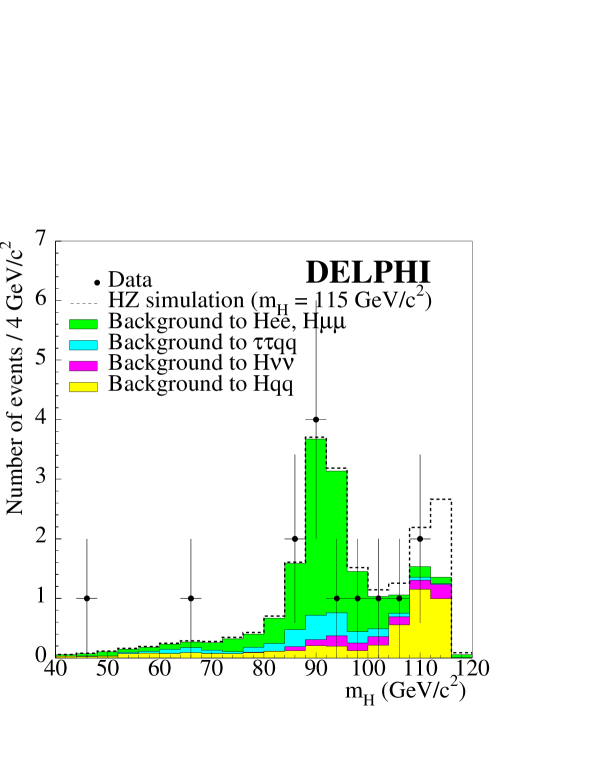
Figure 21: Distribution of the reconstructed SM Higgs boson masses for the tightly selected candidates in each channel from the 2000 data. Data (dots) are compared with background process expectations (full histograms) and with the normalised signal spectrum added to the background channel contributions (dashed histogram). The mass hypothesis for the simulated signal spectrum is $m_{\mathrm{H}}\,$ = 115 ${\mathrm{GeV}}/c^{2}$.

There are three events with a signal to background ratio higher than 0.2 for the hypothesis $m_{\mathrm{H}}\,$ = 115 ${\mathrm{GeV}}/c^{2}$; all are four-jet Higgs boson candidates. Two of them have reconstructed Higgs boson mass above 105 ${\mathrm{GeV}}/c^{2}$ while the other has mass $97.4$ ${\mathrm{GeV}}/c^{2}$. The value from the ANN is higher than 0.8 for all three events, which were all collected at a centre-of-mass energy of 206.6 ${\mathrm{GeV}}$. The first candidate was reconstructed with a Higgs boson mass of 110.7 ${\mathrm{GeV}}/c^{2}$ and with an ANN value of 0.85. The pairing selected corresponds to jet pair masses after the 4C fit (i.e. before the Z mass is fixed to its central value) of 105.1 and 96.8 ${\mathrm{GeV}}/c^{2}$. In the high mass jet pair one of the jets has a high ${\mathrm{b}}$-tagging value with a clear secondary vertex; in the low mass jet pair there is also a jet with a high ${\mathrm{b}}$-tagging value. The third and fourth jets, ordered by ${\mathrm{b}}$-tagging, have values which have probabilities of 25$\%$ and 67$\%$ to occur in a four-b event. The second candidate was reconstructed with a Higgs boson mass of 108.2 ${\mathrm{GeV}}/c^{2}$ and with an ANN of 0.83. The pairing selected corresponds to jet pair masses of 113.1 and 87.1 ${\mathrm{GeV}}/c^{2}$. The two jets of the low mass jet pair have high ${\mathrm{b}}$-tag values with a secondary vertex in each jet. The third candidate was reconstructed with a Higgs boson mass of 97.4 ${\mathrm{GeV}}/c^{2}$ and with an ANN of 0.96, the highest of all the events collected in year 2000. The two pairings with lowest $\chi^{2}$, after a 5C fit with the Z mass fixed, had $\chi^{2}$ values of 3.58 and 3.97; they correspond to Higgs boson mass estimators of 113.4 ${\mathrm{GeV}}/c^{2}$ and 97.4 ${\mathrm{GeV}}/c^{2}$. After applying the algorithm described in section 9.1 the second one was selected. The jet pair masses for such a pairing were 101.3 and 87.0 ${\mathrm{GeV}}/c^{2}$. The two jets of the high mass pairing had high ${\mathrm{b}}$-tag values with one clear secondary vertex in each jet, while the jets of the low mass jet pair had ${\mathrm{b}}$-tagging values which have probabilities of 34$\%$ and 56$\%$ to occur in a four-b event.

The events selected by a tight cut in the MSSM Higgs boson search are shown in Fig. 22. The cut has been made on the second discriminant variable such that a signal might be more apparent. The selections require a minimal likelihood value of 0.90 in the $\tau^{+}\tau^{-}{\mathrm{q}\bar{q}}$   channel, and a minimal neural network output of 0.95 in the ${\mathrm{b}}\bar{\mathrm{b}}$${\mathrm{b}}\bar{\mathrm{b}}$ channel. Both the 2000 and 1999 results are included. The analysis of the $\tau^{+}\tau^{-}{\mathrm{q}\bar{q}}$  channel for 1999 is taken from our previous publication [1] for completeness. The corresponding observed and expected rates in each period are given in Table 8, which can be compared with Table 5.

Channel	Data	Total	${\mathrm{q}}\bar{\mathrm{q}}(\gamma)$	4 fermion	Efficiency (%)
		background
1999 data, 191.6 - 201.7 ${\mathrm{GeV}}$
Tau	0	0.78$\pm$0.06	0.13	0.65	12.8
Four-jet	6	7.82$\pm$0.2	1.7	5.7	55.0
First period 2000
Tau	0	0.4$\pm$0.05	0.04	0.38	11.5
Four-jet	7	5.7$\pm$0.2	1.7	4.1	55.0
Second period 2000
Tau	0	0.11$\pm$0.03	0.01	0.11	11.0
Four-jet	3	1.8$\pm$0.06	0.41	1.36	50.3

Table 8: Candidates selected for the MSSM channels by tight cuts on data and simulated background processes. The last column gives the efficiencies at a mass $m_{\mathrm{h}}$= $m_{\mathrm{A}}$= 90 ${\mathrm{GeV}}/c^{2}$. The tau results from 1999 are taken from our previous publication.

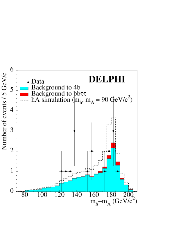
Figure 22: Distribution of the sum of the reconstructed Higgs boson masses for the tight candidates in the ${\mathrm{h}}{\mathrm{A}}$ channels in the 1999 and 2000 data. Data (dots) are compared with SM background process expectations (full histograms) and with the normalised signal spectrum added to the background channel contributions (dashed histogram). The mass hypothesis for the simulated signal spectrum is $m_{\mathrm{h}}$=$m_{\mathrm{A}}$ = 90 ${\mathrm{GeV}}/c^{2}$.

The three events with highest significance for the hypothesis $m_{\mathrm{A}}$=90 ${\mathrm{GeV}}/c^{2}$ at $\tan\beta$ = 20.6 (corresponding to $m_{\mathrm{h}}$ $\sim$90 ${\mathrm{GeV}}/c^{2}$) are described below. The three events are from the 4b channel.

The first event, collected at a centre-of-mass energy of 206.6 ${\mathrm{GeV}}$, is reconstructed with a sum of Higgs boson masses of 120.9 ${\mathrm{GeV}}/c^{2}$ and with an ANN of 0.99. Its content in b-quarks is high, the jet with the lowest ${\mathrm{b}}$-tag value having a probability of 70% to have such a value in a four-b event. However, in the three possible jet pairings, the mass difference between any two jet pairs is well within the resolution expected on this variable. The differences are 8.8, 4.4, and 5.1 ${\mathrm{GeV}}/c^{2}$, corresponding to a sum of masses of 178.2, 120.9 and 202.3 ${\mathrm{GeV}}/c^{2}$, respectively. If instead of the minimal mass difference between the two jet pairs, the $\chi^{2}$ of a five-constraint fit imposing equal masses of the two jet pairs is used as a criterion to pair the jets, the high mass solution would be selected with a $\chi^{2}$ of 5.7, while the low mass solution has a $\chi^{2}$ of 7.0 and the third combination, the one closest to the $ZZ$ hypothesis, has a $\chi^{2}$ of 7.9. Although this event appears to be a good 4b candidate, it has an ambiguity in the mass estimation which allows an almost equally good interpretation as an on-shell ${\mathrm{ZZ}}$ candidate, or as a ${\mathrm{ZZ}}$^∗ candidate with the Z^∗ far below or above its nominal mass.

The second event, collected at a centre-of-mass energy of 205.1 ${\mathrm{GeV}}$, is reconstructed with a sum of Higgs boson masses of 180.5 ${\mathrm{GeV}}/c^{2}$ and with an ANN of 0.97. The jet pairings which are not selected have a much larger $\chi^{2}$ for an equal mass hypothesis than that which is used, suggesting that the event is likely to be due to ${\mathrm{ZZ}}$ production.

The third event, taken at a centre-of-mass energy of 206.6 ${\mathrm{GeV}}$ is reconstructed with a sum of Higgs boson masses of 178.6 ${\mathrm{GeV}}/c^{2}$ and with an ANN of 0.96. It has three well reconstructed secondary vertices, which explains the high value of the jet ${\mathrm{b}}$-tagging variables and hence that of ANN. However, as in the first candidate, it has two pairings almost equally probable, with mass differences of 9.3 and 19.4 ${\mathrm{GeV}}/c^{2}$, corresponding to a sum of masses of 178.6 and 201.9 ${\mathrm{GeV}}/c^{2}$, respectively. The $\chi^{2}$ of a five-constraint fit is 14.3 for the pairing close to the ${\mathrm{ZZ}}$ hypothesis, and 14.5 for the high-mass solution.

11.2 The SM Higgs boson

Confidence levels as a function of the SM Higgs boson mass are derived, combining the data analysed in the previous sections with those taken at energies from 161.0 to 202 ${\mathrm{GeV}}$ [31, 5, 25, 1]. The expected cross-sections and branching ratios are taken from the database provided by the LEP Higgs working group, using the HZHA [15] package with the top mass set to 174.3 ${\mathrm{GeV}}/c^{2}$. As noted earlier, the H$\nu\bar{\nu}$ and $\mbox{H}{\mathrm{q\bar{q}}}$ channels each use two analyses, one for most of the range and the other optimised for the kinematic limit. The selection between these is done independently for each energy window and each mass hypothesis under consideration.

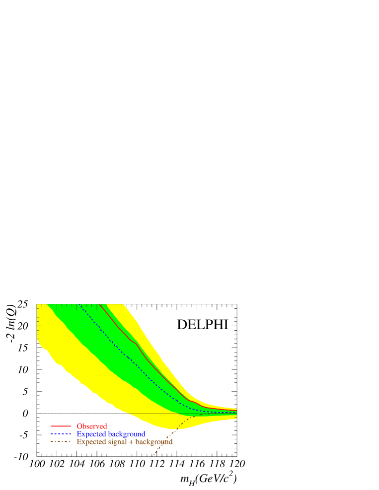
Figure 23: SM Higgs boson: test-statistic $-2\ln\mbox{$\cal Q$}$ for each $m_{\mathrm{H}}\,$ hypothesis in data (solid) and its expected median value in background-only experiments (dashed). The bands correspond to the 68.3% and 95.0% confidence intervals from experiments with only background processes. The dash-dotted curve shows the expected mean value if a signal were present; the error bands on this would be rather similar in width to those on the background-only curve at the same mass.

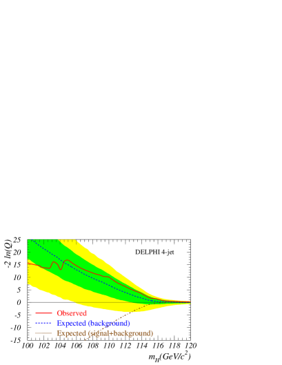
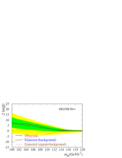
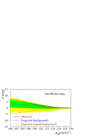
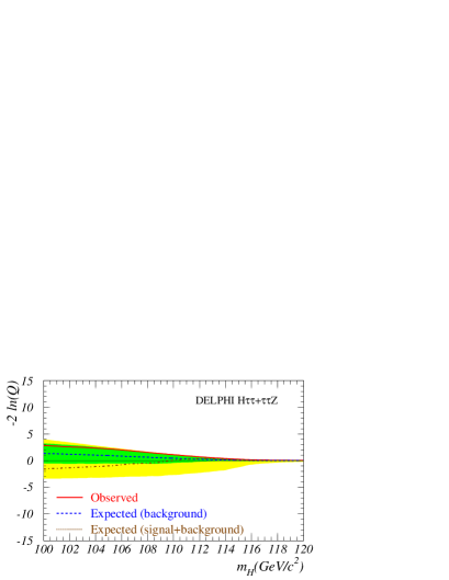
Figure 24: SM Higgs boson: test-statistic $-2\ln\mbox{$\cal Q$}$ for each $m_{\mathrm{H}}\,$ hypothesis in four channels: hadronic, H$\nu\bar{\nu}$, Hll and channels with tau leptons. The conventions are as in figure 23. No channel produces a signal-like result at any mass.

The curve of the test-statistic $\cal Q$ as a function of the mass hypothesis is shown in Fig. 23, where the observation is compared with the xpectations from experiments with only background processes and from experiments where both signal and background channels exist. Over the whole range of masses, the test-statistic remains positive, while in the event of a discovery it would be negative for mass hypotheses close to the actual mass of the signal.

The same curve is shown in Fig. 24, except that the test-statistic $\cal Q$ is broken into 4 channels, four jets, H$\nu\bar{\nu}$, H${\mathrm{e^{+}e^{-}}}$ plus H$\mu^{+}\mu^{-}$ and tau channels. In the region abouve 110 ${\mathrm{GeV}}/c^{2}$ the H$\nu\bar{\nu}$ channel has a result which is median for background, while the other three have a slight deficit compared with the background, of the order of one sigma.

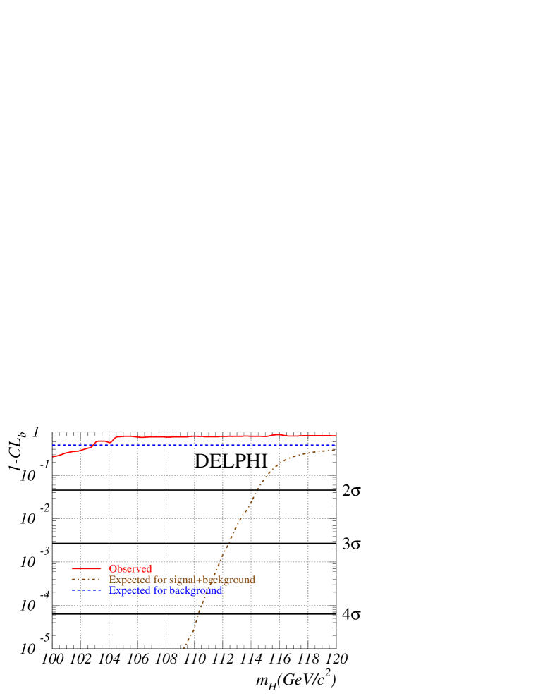
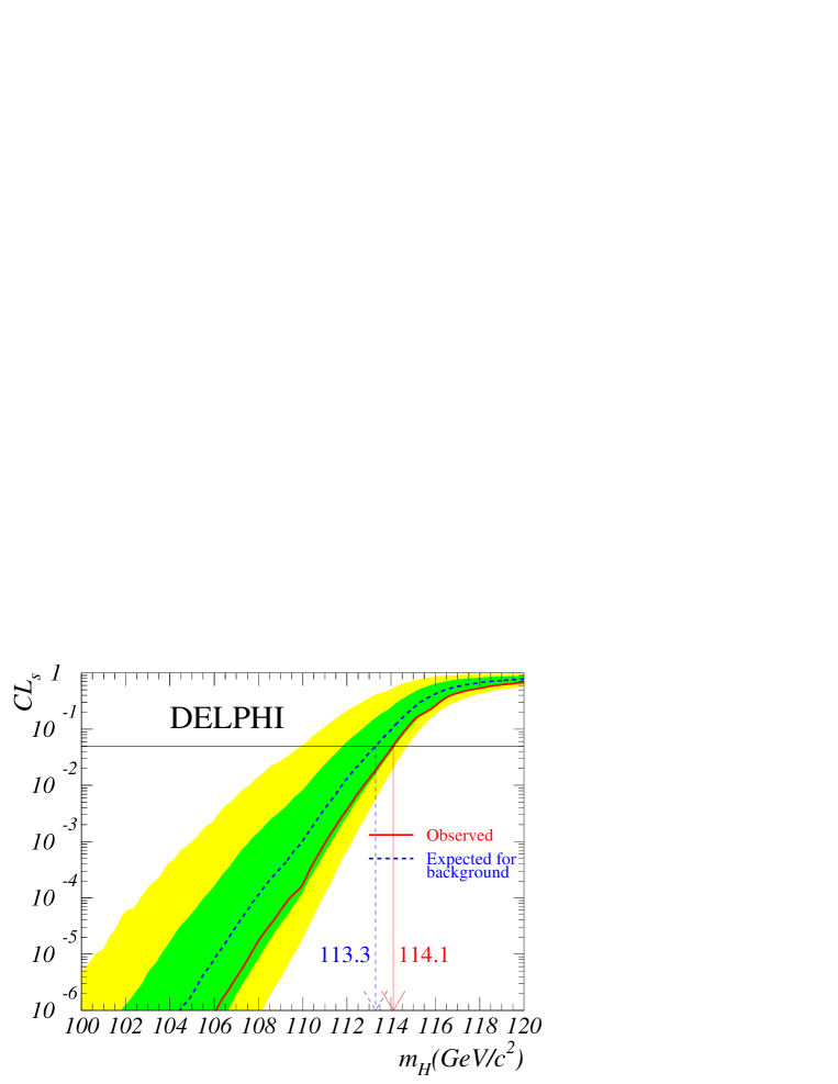
Figure 25: SM Higgs boson: confidence levels as a function of $m_{\mathrm{H}}\,$. Top: 1-$\rm CL_{\rm b}$  for the background hypothesis. The full curve is the observation, the dashed curve is the median expected for background only, and the dash-dotted curve is the median expected at a particular $m_{\mathrm{H}}\,$ value when tested for that $m_{\mathrm{H}}\,$value. A signal would appear as a downward deviation. Bottom: $\rm CL_{\rm s}$, the pseudo-confidence level for the signal hypothesis. Curves are the observed (full) and expected median (dashed) confidences from experiments with only background channels while the bands correspond to the 68.3% and 95.0% confidence intervals for the hypothesis of only background processes. The intersections of the curves with the horizontal line at 5% define the expected and observed 95% CL lower limits on $m_{\mathrm{H}}\,$.

Curves of the confidence level $\rm CL_{\rm b}$ and $\rm CL_{\rm s}$ (as defined in section 4.5) as a function of the test mass $m_{\mathrm{H}}\,$ are shown in Fig. 25. In the presence of a sizable Higgs signal, the value of the observed $\rm CL_{\rm b}$ (top of Fig. 25) would approach one, since it measures the fraction of experiments with only background processes which are more background-like than the observation. Here the compatibility between the observation and the expectation from background processes is well within one standard deviation over the range of masses tested. The pseudo-confidence level in the signal is shown in Fig. 25 (bottom). The observed 95% CL lower limit on the mass is 114.1 ${\mathrm{GeV}}/c^{2}$ while the expected median limit is $113.3~{}\mbox{${\mathrm{GeV}}/c^{2}$}$. If the Higgs boson mass was below 107.5 ${\mathrm{GeV}}/c^{2}$ this search would produce an expected 5$\sigma$ discovery; all such masses are instead excluded at 99.999% CL or better.

It is possible to calculate the Bayesian credibility of these (essentially frequentist) 95% CL limits. This is the probability that our results are correct, that is to say that the true Higgs boson mass is greater than our limit. Like any Bayesian probability this needs a prior belief. Working within the framework of the Standard Model two interesting priors are to take a probability flat in $\log m_{H}$ up to 1 TeV, or the same but modified by the electroweak fits results as they are currently known [32] (i.e. $m_{H}=81^{+52}_{-33}$). The posterior probability density function is obtained by multiplying the prior by the likelihood distribution from this experiment and normalising. The credibilities when integrating from the quoted limit to 1 TeV are 99.97% for the flat case and 99.8% when the electroweak fit results are considered. These probabilities, of course, assume that there is exactly one Standard Model Higgs. By construction the $\rm CL_{\rm s}$ method will always produce large credibilities.

11.3 Limits on the H coupling to Z(W)

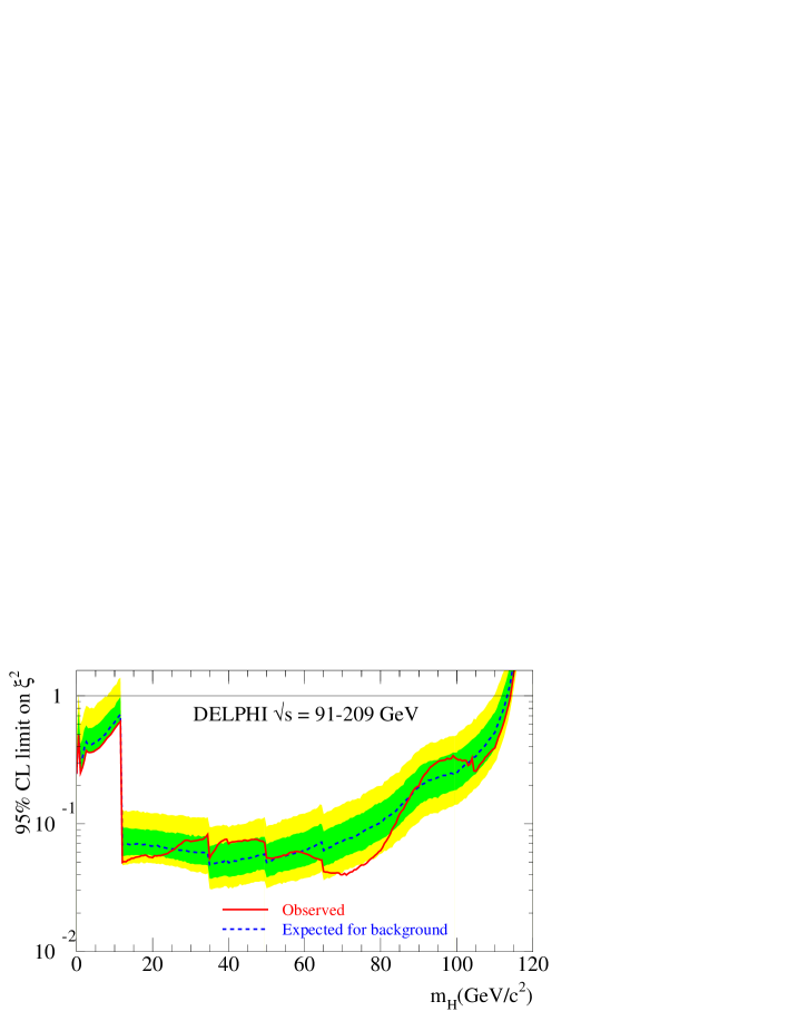
Figure 26: 95% CL upper bound on $\xi^{2}$, where $\xi$ is the HVV (V=${\mathrm{W}}^{\pm}\,$ or Z) coupling normalised to that in the SM, assuming SM branching fractions for the Higgs boson. The limit observed in data (full curve) is shown together with the expected median limit in background process experiments (dashed curve). The bands correspond to the 68.3% and 95.0% confidence intervals from background-only experiments. The limits are significantly less stringent below 12 ${\mathrm{GeV}}/c^{2}$, the ${\mathrm{b}}\bar{\mathrm{b}}$ threshold, where only results obtained on subsets of the LEP 1 data are used.

In a more general approach, the results of the searches for a SM Higgs boson can be used to set a 95% CL upper bound on the Higgs boson production as a function of its mass. Here it is assumed that the Higgs boson decay properties are identical to those in the SM but that the Higgs boson couplings to pairs of Z and ${\mathrm{W}}^{\pm}\,$ bosons (the latter arising in the ${\mathrm{W}}^{+}{\mathrm{W}}^{-}$ fusion production mechanism) may be smaller. To achieve the best sensitivity over the widest range of mass hypotheses, the results described in this paper are combined consistently with those obtained at lower energies at LEP2 [1, 25, 5, 31], as well as with those obtained at LEP1 [33] which covered masses up to 60 ${\mathrm{GeV}}/c^{2}$. For each mass hypothesis, the production cross-section is decreased with respect to its SM value until a pseudo-confidence level $\rm CL_{\rm s}$ of 5% is obtained.

The coupling $\xi$ is introduced as the HVV (V=${\mathrm{W}}^{\pm}\,$ or Z) coupling normalised to that in the SM, assuming SM branching fractions for the Higgs. In practice, $\xi$ is dominated by the HZZ coupling. The 95% CL upper bound on $\xi^{2}$ is shown in Fig. 26 for masses of the Higgs boson from 0 to 120 ${\mathrm{GeV}}/c^{2}$. The SM result described in the previous section corresponds to a ratio of 1.

11.4 Neutral Higgs bosons in the MSSM

The results in the ${\mathrm{h}}{\mathrm{Z}}$ and ${\mathrm{h}}{\mathrm{A}}$ channels reported in the previous sections are combined with the same statistical method as for the SM, also using earlier results at LEP2 energies [1, 25, 5, 31, 34], to derive confidence levels in scans of the MSSM parameter space. The exclusion limits obtained at LEP1 [35] ($m_{\mathrm{h}}$$>$44 (46) ${\mathrm{GeV}}/c^{2}$ when $m_{\mathrm{h}}$ is above (below) the ${\mathrm{AA}}$ threshold) are used as external constraints to limit the number of points in the scans.

11.4.1 The benchmark scenarios

At tree level, the production cross-sections and the Higgs branching fractions in the MSSM depend on two free parameters, $\tan\beta$ and one Higgs boson mass, or, alternatively, two Higgs boson masses, e.g. $m_{\mathrm{A}}$ and $m_{\mathrm{h}}$. Radiative corrections introduce additional parameters related to supersymmetry breaking. Hereafter, the usual assumption that some of them are identical at a given energy scale is made: hence, the SU(2) and U(1) gaugino mass terms are assumed to be unified at the so-called GUT scale, while the sfermion mass terms or the squark trilinear couplings are assumed to be unified at the EW scale. Within these assumptions, the parameters beyond tree level are: the top quark mass, the Higgs mixing parameter, $\mu$, the common sfermion mass term at the EW scale, $M_{\rm susy}$, the SU(2) gaugino mass term at the EW scale, $M_{2}$, the gluino mass, $m_{\tilde{g}}$, and the common squark trilinear coupling at the EW scale, $A$. The U(1) gaugino mass term at the EW scale, $M_{1}$, is related to $M_{2}$ through the GUT relation $M_{1}=(5/3){\rm\tan}^{2}\theta_{W}M_{2}$. The radiative corrections affect the relationships between the masses of the Higgs bosons, with the largest contributions arising from the top/stop loops. As an example, the h boson mass, which is below that of the Z boson at tree level, increases by a few tens of ${\mathrm{GeV}}/c^{2}$ in some regions of the MSSM parameter space due to radiative corrections.

scenario	$m_{\mathrm{t}op}$	$M_{\rm susy}$	$M_{2}$	$m_{\tilde{g}}$	$\mu$	$X_{t}$
	(${\mathrm{GeV}}/c^{2}$)	(${\mathrm{GeV}}/c^{2}$)	(${\mathrm{GeV}}/c^{2}$)	(${\mathrm{GeV}}/c^{2}$)	(${\mathrm{GeV}}/c^{2}$)	(${\mathrm{GeV}}/c^{2}$)
$m_{\mathrm{h}}^{\rm max}$ scenario	174.3	1000	200	800	-200	2 $M_{\rm susy}$
no-mixing	174.3	1000	200	800	-200	0
large $\mu$	174.3	400	400	200	1000	-300

Table 9: Values of the underlying parameters for the three representative MSSM scenarios scanned in this paper. Note that $X_{t}$ is $A-\mu\cot\beta$.

In the following, three benchmark scenarios are considered, as suggested in Ref. [36]. These are quite representative since the limits obtained in these schemes with earlier results were only slightly reduced in more general parameter scans [1]. The first two scenarios, called the $m_{\mathrm{h}}^{\rm max}$ scenario and the no-mixing scenario, rely on radiative corrections computed at partial two-loop order as in Ref.[37]. The values of the underlying parameters are quoted in Table 9. The two scenarios differ only by the value of $X_{t}=A-\mu\cot\beta$, the parameter which controls the mixing in the stop sector, and hence has the largest impact on the mass of the h boson. The $m_{\mathrm{h}}^{\rm max}$ scenario leads to the maximum possible h mass as a function of $\tan\beta$. The no-mixing scenario is its counterpart with vanishing mixing, leading to upper bounds on $m_{\mathrm{h}}$ which are at least 15 ${\mathrm{GeV}}/c^{2}$ lower than in the $m_{\mathrm{h}}^{\rm max}$ scheme.

The third scenario, called the large $\mu$ scenario, predicts at least one scalar Higgs boson with a mass within kinematic reach at LEP2 in each point of the MSSM parameter space. However, there are regions for which the Higgs bosons cannot be detected because of vanishing branching fractions into b-quarks. In this scenario, the radiative corrections are computed as in Ref. [38]. The values of the underlying parameters are given in Table 9. The main difference with the two previous schemes is the large and positive value of $\mu$ and the relatively small value of $m_{\tilde{g}}$.

It must be noted that, with respect to the calculations of Ref. [37, 38] used in this paper, recent theoretical improvements exist that include more complete two-loop order radiative corrections and a redefinition of the underlying parameters of the benchmark scenarios, that lead in particular to an extended allowed range of the h boson mass Ref. [39]. These changes will probably reduce the excluded region in $\tan\beta$.

11.4.2 The procedure

In the three benchmark scenarios, a scan was performed over the MSSM parameters $\tan\beta$ and $m_{\mathrm{A}}$. The range in $m_{\mathrm{A}}$ spans from 12 ${\mathrm{GeV}}/c^{2}$, the minimal value which has been searched for at LEP2 in the DELPHI analyses, up to the maximal value allowed by each scenario [36], that is up to $M_{\rm susy}$, which is 1 TeV/$c^{2}$ in the $m_{\mathrm{h}}^{\rm max}$ and no-mixing schemes, and 400 ${\mathrm{GeV}}/c^{2}$ in the large $\mu$ scenario (see Table 9). The range in $\tan\beta$ extends from the minimal value allowed in each scenario up to 50, a value chosen in the vicinity of the ratio of the top- and b-quark masses, which is an example of the large $\tan\beta$ hypothesis favoured in some constrained MSSM models [40]. The scan steps were 1 ${\mathrm{GeV}}/c^{2}$ in $m_{\mathrm{A}}$ and 0.1 in $\tan\beta$ in the regions where $m_{\mathrm{h}}$ varies rapidly with these parameters.

At each point of the parameter space, the ${\mathrm{h}}{\mathrm{Z}}$ and ${\mathrm{h}}{\mathrm{A}}$ cross-sections and the Higgs branching fractions were taken from databases provided by the LEP Higgs working group, Ref. [41], on the basis of the theoretical calculations in Refs. [37, 38]. The signal expectations in each channel were then derived from the theoretical cross-sections and branching fractions, the experimental luminosity and the efficiencies. A correction was applied to account for different branching fractions of the Higgs bosons into ${\mathrm{b}}\bar{\mathrm{b}}$ and $\tau^{+}\tau^{-}$ between the test point and the simulation (e.g. for the ${\mathrm{h}}{\mathrm{Z}}$ process, the simulation was done in the SM framework). For the hA channels, to account for non-negligible widths of the h and A bosons at large $\tan\beta$ the set of efficiencies from the $m_{\mathrm{h}}$, $m_{\mathrm{A}}$ simulations was applied for $\tan\beta$ $<$ 30. Above that value, efficiencies were linearly interpolated in $\tan\beta$ between the efficiencies from the $m_{\mathrm{h}}$, $m_{\mathrm{A}}$ simulations and those from the simulations at $\tan\beta$ = 50. As the Higgs boson widths grow approximately linearly with $\tan\beta$ above 30, a linear interpolation is valid. The same holds for the discriminant information, for which the same interpolation software was used as discussed in section 4.5 for the PDF interpolation in mass or centre-of-mass energy.

Finally, when combining the results in all channels to derive confidence levels, only independent channels must be included, which requires some special treatment for a few non-independent cases. As already mentioned in section 7, the four $\tau^{+}\tau^{-}$${\mathrm{q}}\bar{\mathrm{q}}$ signals, which were covered by the same analysis, were thus combined into one global $\tau^{+}\tau^{-}$${\mathrm{q}}\bar{\mathrm{q}}$ channel prior to the confidence level computation. The same applies to the four signals selected by the low mass ${\mathrm{h}}{\mathrm{Z}}$ four-jet analysis - the $\mbox{h}{\mathrm{q\bar{q}}}$ signal, the two (${\mathrm{h}}\rightarrow{\mathrm{AA}}$)(${\mathrm{Z}}\rightarrow$ ${\mathrm{q}}\bar{\mathrm{q}}$) signals and the 4b signal (see section 9.3) - or to the two signals selected by the ${\mathrm{h}}{\mathrm{A}}$ four-b analysis - the 4b signal and the $\mbox{h}{\mathrm{q\bar{q}}}$ signal (see section 9.3). Moreover, in three cases, there was also a large overlap in the events selected by two different analyses: the low and high mass analyses in the missing energy channel or in the four-jet ${\mathrm{h}}{\mathrm{Z}}$ channel and the four-jet ${\mathrm{h}}{\mathrm{Z}}$ and ${\mathrm{h}}{\mathrm{A}}$ analyses. In each case, only one of the two analyses was selected at each input point and at each centre-of-mass energy, on the basis of the smallest expected $\rm CL_{\rm s}$ from experiments with no signal (that is, on the basis of the strongest average exclusion if no signal is present). This ensures that the channels which are then combined in the global confidence level computations are independent.

11.4.3 Consistency tests in the ${\mathrm{h}}{\mathrm{A}}$ channels

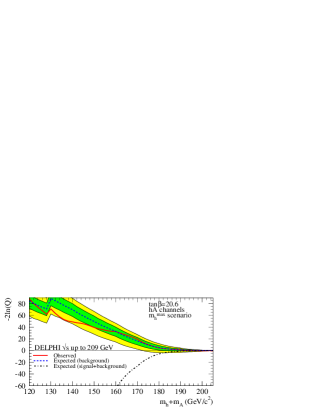
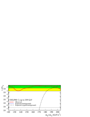
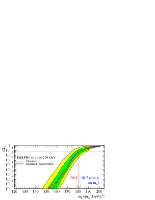
Figure 27: hA analyses: test-statistic (top) and confidence levels in the background-only hypothesis (middle) and in signal hypothesis (bottom) as functions of $m_{\mathrm{h}}$+$m_{\mathrm{A}}$. Curves are the observed (full) and median expected (dashed) results from background-only experiments while the bands correspond to the 68.3% and 95.0% confidence intervals from the latter. The dash-dotted curves are the expected mean values from experiments where a signal of mass given in the abscissa is added to the background. The limited range of the results derived at 188.7 ${\mathrm{GeV}}/c^{2}$ explains the hook at 130 ${\mathrm{GeV}}/c^{2}$ in the top plot.

Fig. 27 shows the curves of the test-statistic $\cal Q$ and of the confidence levels $\rm CL_{\rm b}$ and $\rm CL_{\rm s}$ as a function of the test mass $m_{\mathrm{h}}$+$m_{\mathrm{A}}$, when using only the results of the two ${\mathrm{h}}{\mathrm{A}}$ analyses applied onto the two ${\mathrm{h}}{\mathrm{A}}$ signals. The signal cross-sections are from the $m_{\mathrm{h}}^{\rm max}$ scenario at $\tan\beta$ = 20.6. Over the whole range of test masses, data are in reasonable agreement with the background process expectations. For test masses $m_{\mathrm{h}}$+$m_{\mathrm{A}}$ around 135 ${\mathrm{GeV}}/c^{2}$ a two standard deviation effect is observed which is due to the small excess of events in the 4b channel with reconstructed masses in that region, as seen in Fig. 22. The mass resolution is around 5 ${\mathrm{GeV}}/c^{2}$, and therefore the region 120 to 205 ${\mathrm{GeV}}/c^{2}$ shown contains some 15 or 20 effectively independent points, and therefore it is not surprising that there is a deviation of this magnitude at some mass. There is a small excess, only just over one sigma, at 200 ${\mathrm{GeV}}/c^{2}$, which is not apparent in Fig. 22. It involves only 2 significant events with reconstructed mass greater than 200 ${\mathrm{GeV}}/c^{2}$, and these have NN values of 0.94 and 0.93 respectively, and so do not appear in the mass plot.

Furthermore, the $\rm CL_{\rm s}$ curves show that, in the particular scenario under study, the exclusion limits on $m_{\mathrm{h}}$+$m_{\mathrm{A}}$, both observed and expected, are around 181 ${\mathrm{GeV}}/c^{2}$. The exclusion and discovery potentials rise fast when testing mass hypotheses below that value. As an example, the 5 sigma discovery potential reaches 171 ${\mathrm{GeV}}/c^{2}$ in $m_{\mathrm{h}}$+$m_{\mathrm{A}}$(see 1-$\rm CL_{\rm b}$ curves), only 10 ${\mathrm{GeV}}$ below the limit at 95% CL, and this sum of masses is experimentally excluded with a $\rm CL_{\rm s}$ of $10^{-4}$ (see $\rm CL_{\rm s}$ curves).

11.4.4 Exclusion regions

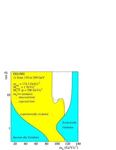
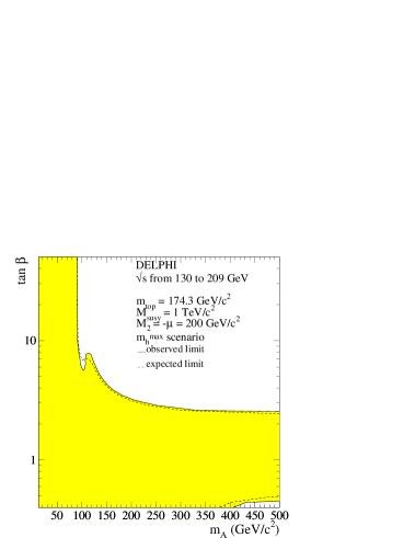
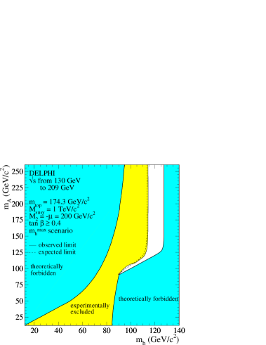
Figure 28: MSSM Higgs bosons: regions excluded at 95% CL by the searches in the combined ${\mathrm{h}}{\mathrm{Z}}$ and ${\mathrm{h}}{\mathrm{A}}$ channels, in the $m_{\mathrm{h}}^{\rm max}$ scenario. The dark shaded areas are the regions not allowed by the MSSM model in this scenario. The dashed curves show the median expected limits.

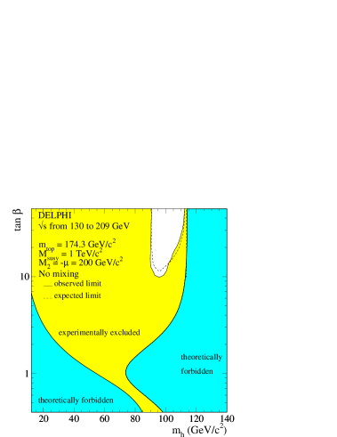
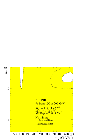
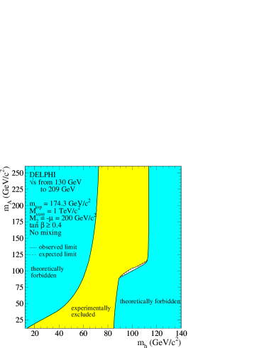
Figure 29: MSSM Higgs bosons: regions excluded at 95% CL by the searches in the combined ${\mathrm{h}}{\mathrm{Z}}$ and ${\mathrm{h}}{\mathrm{A}}$ channels, in the no-mixing scenario. The dark shaded areas are the regions not allowed by the MSSM model in this scenario. The dashed curves show the median expected limits.

Combining the results in the ${\mathrm{h}}{\mathrm{Z}}$ and ${\mathrm{h}}{\mathrm{A}}$ channels gives regions of the MSSM parameter space which are excluded at 95% CL or more. The excluded regions in the ($m_{\mathrm{h}}$, $\tan\beta$), ($m_{\mathrm{A}}$, $\tan\beta$) and ($m_{\mathrm{h}}$, $m_{\mathrm{A}}$) planes are presented in Fig. 28 for the $m_{\mathrm{h}}^{\rm max}$ scenario and in Fig. 29 for the no-mixing scenario. For $m_{\mathrm{A}}$ below the kinematic threshold $m_{\mathrm{h}}$ = 2$m_{\mathrm{A}}$, which occurs at low $\tan\beta$ only, the decay h$\rightarrow$AA opens, in which case it supplants the h$\rightarrow$${\mathrm{b}}\bar{\mathrm{b}}$ decay. However, in most of the region, the A$\rightarrow$${\mathrm{b}}\bar{\mathrm{b}}$ and A$\rightarrow$${\mathrm{c}}\bar{\mathrm{c}}$ branching fractions are large which explains why the results in the (${\mathrm{h}}\rightarrow{\mathrm{AA}}$) ${\mathrm{q}}\bar{\mathrm{q}}$ channels reported in section 9.3, combined with studies of the ${\mathrm{h}}\rightarrow{\mathrm{AA}}$ decay at lower energies [1, 5, 31], exclude this region in both scenarios.

The above results establish 95% CL lower limits on $m_{\mathrm{h}}$ and $m_{\mathrm{A}}$, for either assumption on the mixing in the stop sector and for all values of $\tan\beta$ above 0.4:

$$\mbox{$m_{\mathrm{h}}$}>89.7~{}\mbox{${\mathrm{GeV}}/c^{2}$}\hskip 28.45274pt\mbox{$m_{\mathrm{A}}$}>90.4~{}\mbox{${\mathrm{GeV}}/c^{2}$}.$$

The expected median limits are 90.6 ${\mathrm{GeV}}/c^{2}$ for $m_{\mathrm{h}}$ and 90.5 ${\mathrm{GeV}}/c^{2}$ for $m_{\mathrm{A}}$. The limit in $m_{\mathrm{A}}$ is reached in the no-mixing scenario at $\tan\beta$ around 30, that is in a region where Higgs bosons have non-negligible widths, while the limit in $m_{\mathrm{h}}$ is obtained in the $m_{\mathrm{h}}^{\rm max}$ scenario at $\tan\beta$ around 10, in a region where both the ${\mathrm{h}}{\mathrm{Z}}$ and ${\mathrm{h}}{\mathrm{A}}$ processes contribute. Furthermore, there are excluded ranges in $\tan\beta$ between 0.4 and 9.36 (expected [0.4-9.36]) in the no-mixing case and between 0.54 and 2.36 (expected [0.54-2.14]) in the $m_{\mathrm{h}}^{\rm max}$ scenario. Note that in the case of no-mixing, while the observed and expected lower limits on $\tan\beta$ are the same, they appear at quite different A and h masses.

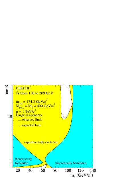
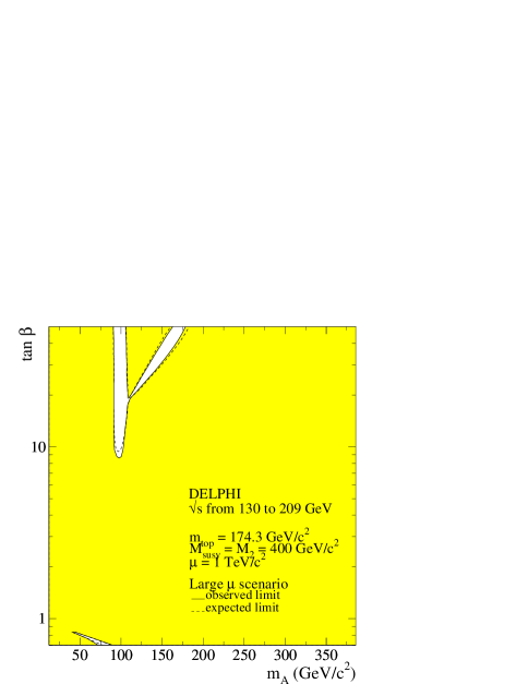
Figure 30: MSSM Higgs bosons: regions excluded at 95% CL, by the searches in the combined ${\mathrm{h}}{\mathrm{Z}}$ and ${\mathrm{h}}{\mathrm{A}}$ channels, in the large $\mu$ scenario. The dark shaded areas are the regions not allowed by the MSSM model in this scenario. The dashed curves show the median expected limits.

The excluded regions in the large $\mu$ scenario are presented in the ($m_{\mathrm{h}}$, $\tan\beta$) and ($m_{\mathrm{A}}$, $\tan\beta$) planes in Fig. 30. A large fraction of the allowed domain is excluded by the present results in the ${\mathrm{h}}{\mathrm{Z}}$ and ${\mathrm{h}}{\mathrm{A}}$ channels. In particular, given that the theoretical upper bound on the h boson mass in that scenario is slightly above 107 ${\mathrm{GeV}}/c^{2}$, the sensitivity of the ${\mathrm{h}}{\mathrm{Z}}$ channels is high even at large $\tan\beta$, which explains why the excluded region reaches the theoretically forbidden area for large values of $\tan\beta$. On the other hand, there is an unexcluded hole in the low $\tan\beta$ region at $m_{\mathrm{h}}$ around 60 ${\mathrm{GeV}}/c^{2}$ which is due to a loss of sensitivity because of vanishing h$\rightarrow$${\mathrm{b}}\bar{\mathrm{b}}$ branching fractions in that region. The unexcluded area at large $\tan\beta$ is mostly due to low expected rates in the ${\mathrm{h}}{\mathrm{Z}}$ and ${\mathrm{h}}{\mathrm{A}}$ channels (the ${\mathrm{h}}{\mathrm{A}}$ kinematic limit is close and the ZZh coupling is low) rather than to vanishing branching fractions into b’s. At these unexcluded points the second scalar boson, H, is kinematically accessible and has a large branching fraction into b-quarks. Allowing for its production in the scans should lead to an improved sensitivity. There are also points with vanishing branching fractions of the h boson into b-quarks, and it is expected that improvements could be made by allowing for other decay modes, such as gluons or c quarks. These possibilities, and the theoretical scenarios referred to in section 11.4.1, could profitably be explored in a future publication.

11.5 Limits on the coupling between h, A and Z

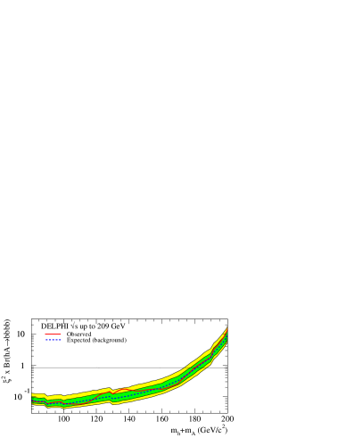
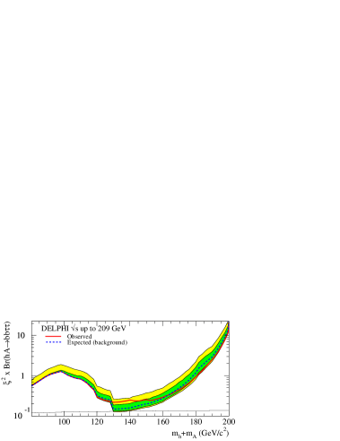
Figure 31: 95% CL upper bounds on $\xi^{2}$, where $\xi$ is the ${\mathrm{h}}{\mathrm{A}}$Z coupling factor normalised to its maximal value in the MSSM, as functions of $m_{\mathrm{h}}$+$m_{\mathrm{A}}$. Results are presented in the ${\mathrm{b}}\bar{\mathrm{b}}$${\mathrm{b}}\bar{\mathrm{b}}$ (top) and ${\mathrm{b}}\bar{\mathrm{b}}$$\tau^{+}\tau^{-}$ (bottom) channels, for nearly mass-degenerate h and A bosons. The limits observed in data (full curve) are shown together with the expected median limits in background process experiments (dashed curve). The bands correspond to the 68.3% and 95.0% confidence intervals from background-only experiments. The large band asymmetry at low mass in the ${\mathrm{b}}\bar{\mathrm{b}}$$\tau^{+}\tau^{-}$ channel reflects the low level of background of the analyses performed in this mass range. The nearly flat thin lines are the values expected in the MSSM $m_{\mathrm{h}}^{\rm max}$ scenario at $\tan\beta$ = 20.6.

As for the ${\mathrm{h}}{\mathrm{Z}}$ process, the results of the searches for pair produced MSSM Higgs bosons can be reinterpreted in a more general approach to set a 95% CL upper bound on the pair production cross-section. This was done separately in the ${\mathrm{b}}\bar{\mathrm{b}}$${\mathrm{b}}\bar{\mathrm{b}}$ and ${\mathrm{b}}\bar{\mathrm{b}}$$\tau^{+}\tau^{-}$ final states, using in each case the analysis dedicated to the channel under study. To achieve the best sensitivity, the results described in this paper are combined consistently with those obtained at lower energies at LEP2 [1, 25, 5, 31, 34]. Only the case of nearly mass-degenerate h and A Higgs bosons is considered since the ${\mathrm{h}}{\mathrm{A}}$ analyses have their highest sensitivity in that case. For each mass hypothesis, the production cross-section is decreased with respect to its value in the MSSM, using the $m_{\mathrm{h}}^{\rm max}$ scenario at $\tan\beta$=20 as a reference, until a pseudo-confidence level $\rm CL_{\rm s}$ of 5% is obtained. Analogously to the SM, the coupling $\xi$, which is the ${\mathrm{h}}{\mathrm{A}}$Z coupling normalised to its maximal value in the MSSM, is used. $\xi$ is related to the underlying MSSM parameters $\beta$ and $\alpha$, the Higgs doublet mixing angle, through the relation: $\xi$ = cos$(\alpha-\beta)$. The results are then expressed in a way independent from the reference scenario, as 95% CL upper bounds on the product of $\xi^{2}$ and the ${\mathrm{h}}{\mathrm{A}}$ branching fractions into the relevant final states. These bounds are given in Fig. 31 for sums of masses of the h and A bosons from 80 to 200 ${\mathrm{GeV}}/c^{2}$.

12 Conclusions

The 224 pb^-1 of data taken by DELPHI at 200 - 209 ${\mathrm{GeV}}$, combined with our lower energy data, sets the lower limit at 95% CL on the mass of the Standard Model Higgs boson at:

$$\mbox{$m_{\mathrm{H}}\,$}>114.1~{}\mbox{${\mathrm{GeV}}/c^{2}$}.$$

The following limits are derived in the framework of the MSSM $m_{\mathrm{h}}^{\rm max}$ and no-mixing scenarios:

$$\mbox{$m_{\mathrm{h}}$}>89.7~{}\mbox{${\mathrm{GeV}}/c^{2}$}\hskip 28.45274pt\mbox{$m_{\mathrm{A}}$}>90.4~{}\mbox{${\mathrm{GeV}}/c^{2}$}.$$

for all values of $\tan\beta$ above 0.4 and assuming $m_{\mathrm{A}}$$>$ 12 ${\mathrm{GeV}}/c^{2}$.

Acknowledgements

We are greatly indebted to our technical collaborators, to the members of the CERN-SL Division for the excellent performance of the LEP collider, and to the funding agencies for their support in building and operating the DELPHI detector.
We acknowledge in particular the support of
Austrian Federal Ministry of Education, Science and Culture, GZ 616.364/2-III/2a/98,
FNRS–FWO, Flanders Institute to encourage scientific and technological research in the industry (IWT), Belgium,
FINEP, CNPq, CAPES, FUJB and FAPERJ, Brazil,
Czech Ministry of Industry and Trade, GA CR 202/99/1362,
Commission of the European Communities (DG XII),
Direction des Sciences de la Mati$\grave{\mbox{\rm e}}$re, CEA, France,
Bundesministerium f$\ddot{\mbox{\rm u}}$r Bildung, Wissenschaft, Forschung und Technologie, Germany,
General Secretariat for Research and Technology, Greece,
National Science Foundation (NWO) and Foundation for Research on Matter (FOM), The Netherlands,
Norwegian Research Council,
State Committee for Scientific Research, Poland, SPUB-M/CERN/PO3/DZ296/2000, SPUB-M/CERN/PO3/DZ297/2000, 2P03B 104 19 and 2P03B 69 23(2002-2004)
JNICT–Junta Nacional de Investigação Científica e Tecnol$\acute{\mbox{\rm o}}$gica, Portugal,
Vedecka grantova agentura MS SR, Slovakia, Nr. 95/5195/134,
Ministry of Science and Technology of the Republic of Slovenia,
CICYT, Spain, AEN99-0950 and AEN99-0761,
The Swedish Natural Science Research Council,
Particle Physics and Astronomy Research Council, UK,
Department of Energy, USA, DE-FG02-01ER41155.

Appendix

We give in detail the efficiencies of the signal selection here.

$m_{\mathrm{H}}\,$	H${\mathrm{e^{+}e^{-}}}$	H$\mu^{+}\mu^{-}$	H$\tau^{+}\tau^{-}$	$\tau^{+}\tau^{-}$Z	H$\nu\bar{\nu}$		$\mbox{H}{\mathrm{q\bar{q}}}$
(${\mathrm{GeV}}/c^{2}$)	channel	channel	channel	channel	Low mass	High mass	channel
First operational period $\sqrt{s}$ = 206.5 ${\mathrm{GeV}}$
12.0	20.6 $\pm$0.6	42.1 $\pm$0.7			21.2 $\pm$0.6
18.0	30.4 $\pm$0.7	50.5 $\pm$0.7			35.1 $\pm$0.7
24.0	37.6 $\pm$0.7	54.7 $\pm$0.7			38.6 $\pm$0.7
30.0	42.2 $\pm$0.7	56.9 $\pm$0.7			39.1 $\pm$0.7	16.2 $\pm$0.5	9.6$\pm$ 0.4
40.0	48.6 $\pm$0.7	62.0 $\pm$0.7			38.8 $\pm$0.7	26.0 $\pm$0.6	18.6$\pm$ 0.6
50.0	51.5 $\pm$0.7	64.2 $\pm$0.7	13. $\pm$0.5	5. $\pm$0.3	42.2 $\pm$0.7	21.5 $\pm$0.6	25.5$\pm$ 0.7
60.0	54.8 $\pm$0.7	64.9 $\pm$0.7	18. $\pm$0.6	12. $\pm$0.5	42.3 $\pm$0.7	12.6 $\pm$0.5	28.8$\pm$ 0.7
70.0	57.7 $\pm$0.7	67.5 $\pm$0.7	20. $\pm$0.6	22. $\pm$0.7	47.5 $\pm$0.7	12.8 $\pm$0.5	28.0$\pm$ 0.7
80.0	57.8 $\pm$0.7	67.9 $\pm$0.7	20. $\pm$0.6	23. $\pm$0.7	54.9 $\pm$0.7	28.0 $\pm$0.6	28.3$\pm$ 0.7
85.0	60.3 $\pm$0.7	68.7 $\pm$0.7	20. $\pm$0.6	24. $\pm$0.7	59.8 $\pm$0.7	40.9 $\pm$0.7	27.3$\pm$ 0.7
90.0	59.3 $\pm$0.7	69.4 $\pm$0.7	19. $\pm$0.6	24. $\pm$0.7	63.5 $\pm$0.7	51.2 $\pm$0.7	27.5$\pm$ 0.7
95.0	60.4 $\pm$0.7	69.4 $\pm$0.7	19. $\pm$0.6	23. $\pm$0.7	65.6 $\pm$0.7	59.5 $\pm$0.7	36.1$\pm$ 0.8
100.0	59.0 $\pm$0.7	69.8 $\pm$0.6	19. $\pm$0.6	21. $\pm$0.6	65.2 $\pm$0.7	63.2 $\pm$0.7	47.0$\pm$ 1.0
105.0	59.8 $\pm$0.7	69.1 $\pm$0.7	18. $\pm$0.6	21. $\pm$0.6	65.8 $\pm$0.7	67.4 $\pm$0.7	54.5$\pm$ 1.1
110.0	60.4 $\pm$0.7	69.1 $\pm$0.7	18. $\pm$0.6	21. $\pm$0.6	64.2 $\pm$0.7	66.6 $\pm$0.7	58.8$\pm$ 1.1
114.0	58.4 $\pm$0.7	67.2 $\pm$0.7	15. $\pm$0.5	19. $\pm$0.6	55.9 $\pm$0.7	58.7 $\pm$0.7	58.2$\pm$ 1.1
115.0	59.0 $\pm$0.7	67.0 $\pm$0.7	14. $\pm$0.5	19. $\pm$0.6	55.3 $\pm$0.7	58.9 $\pm$0.7	56.5$\pm$ 1.1
116.0	56.7 $\pm$0.7	64.5 $\pm$0.7	14. $\pm$0.5	19. $\pm$0.6	55.0 $\pm$0.7	59.3 $\pm$0.7	53.1$\pm$ 1.0
120.0	52.4 $\pm$0.7	56.3 $\pm$0.7	12. $\pm$0.5	18. $\pm$0.6	52.3 $\pm$0.7	57.7 $\pm$0.7	43.6$\pm$ 0.9
Second operational period $\sqrt{s}$ = 206.5 ${\mathrm{GeV}}$
12.0	18.7 $\pm$0.6	44.7 $\pm$0.7			19.6 $\pm$0.6
18.0	29.5 $\pm$0.6	52.7 $\pm$0.7			28.9 $\pm$0.7
24.0	36.5 $\pm$0.7	56.6 $\pm$0.7			33.6 $\pm$0.7
30.0	39.0 $\pm$0.7	59.4 $\pm$0.7			35.0 $\pm$0.7	14.7 $\pm$0.5	8.9$\pm$ 0.4
40.0	43.2 $\pm$0.7	63.1 $\pm$0.7			38.0 $\pm$0.7	25.2 $\pm$0.6	18.2$\pm$ 0.6
50.0	47.7 $\pm$0.7	66.1 $\pm$0.7	12. $\pm$0.5		40.3 $\pm$0.7	20.0 $\pm$0.6	23.6$\pm$ 0.7
60.0	50.2 $\pm$0.7	66.8 $\pm$0.7	18. $\pm$0.6	11. $\pm$0.5	40.7 $\pm$0.7	11.8 $\pm$0.5	26.9$\pm$ 0.7
70.0	52.5 $\pm$0.7	69.7 $\pm$0.7	20. $\pm$0.6	22. $\pm$0.7	44.8 $\pm$0.7	12.3 $\pm$0.5	25.7$\pm$ 0.7
80.0	54.8 $\pm$0.7	70.3 $\pm$0.7	20. $\pm$0.6	23. $\pm$0.7	51.1 $\pm$0.7	26.0 $\pm$0.6	25.8$\pm$ 0.7
85.0	55.8 $\pm$0.7	70.3 $\pm$0.7	19. $\pm$0.6	23. $\pm$0.7	54.5 $\pm$0.7	36.2 $\pm$0.7	26.4$\pm$ 0.7
90.0	53.8 $\pm$0.7	70.1 $\pm$1.1	20. $\pm$0.6	23. $\pm$0.7	60.4 $\pm$0.7	47.6 $\pm$0.7	26.5$\pm$ 0.7
95.0	55.7 $\pm$0.7	70.7 $\pm$1.1	19. $\pm$0.6	23. $\pm$0.7	63.2 $\pm$0.7	57.1 $\pm$0.7	32.5$\pm$ 0.8
100.0	55.0 $\pm$0.7	70.4 $\pm$1.1	19. $\pm$0.6	21. $\pm$0.6	65.1 $\pm$0.7	62.6 $\pm$0.7	44.4$\pm$ 0.9
105.0	55.3 $\pm$0.7	70.2 $\pm$1.1	17. $\pm$0.6	22. $\pm$0.7	64.1 $\pm$0.7	64.8 $\pm$0.7	51.9$\pm$ 1.0
110.0	56.2 $\pm$0.7	68.9 $\pm$1.1	17. $\pm$0.6	19. $\pm$0.6	60.6 $\pm$0.7	63.8 $\pm$0.7	56.9$\pm$ 1.1
114.0	55.9 $\pm$0.7	68.3 $\pm$1.1	15. $\pm$0.5	19. $\pm$0.6	54.3 $\pm$0.7	58.0 $\pm$0.7	55.2$\pm$ 1.1
115.0	55.0 $\pm$0.7	67.1 $\pm$1.1	15. $\pm$0.5	19. $\pm$0.6	53.6 $\pm$0.7	58.1 $\pm$0.7	54.9$\pm$ 1.0
116.0	54.1 $\pm$0.7	64.8 $\pm$1.1	13. $\pm$0.5	18. $\pm$0.6	53.1 $\pm$0.7	57.9 $\pm$0.7	53.1$\pm$ 1.0
120.0	48.2 $\pm$0.7	54.8 $\pm$1.1	12. $\pm$0.5	19. $\pm$0.6	48.9 $\pm$0.7	56.1 $\pm$0.7	42.6$\pm$ 0.9

Table 10: ${\mathrm{HZ}}$ channels: efficiencies (in %) of the selection in the two operational periods, as a function of the mass of the Higgs boson. The quoted errors are statistical only. Only efficiencies higher than 5% are shown.

$m_{\mathrm{A}}$	$m_{\mathrm{h}}$	$\sqrt{s}$ = 199.6 ${\mathrm{GeV}}$	$\sqrt{s}$ = 206.5 ${\mathrm{GeV}}$	$\sqrt{s}$ = 206.5 ${\mathrm{GeV}}$
(${\mathrm{GeV}}/c^{2}$)	(${\mathrm{GeV}}/c^{2}$)		1st period	2nd period
40.0	40.0	17.3 $\pm$ 0.5	11.4 $\pm$ 0.5	11.4 $\pm$ 0.5
50.0	50.0	62.9 $\pm$ 1.1	61.2 $\pm$ 1.1	59.7 $\pm$ 0.9
60.0	60.0	74.4 $\pm$ 1.2	71.7 $\pm$ 1.2	70.0 $\pm$ 0.9
70.0	70.0	78.6 $\pm$ 1.2	77.5 $\pm$ 1.2	76.4 $\pm$ 0.9
80.0	80.0	85.3 $\pm$ 1.3	85.0 $\pm$ 1.3	83.3 $\pm$ 1.1
85.0	85.0	87.3 $\pm$ 1.3	88.9 $\pm$ 1.3	86.8 $\pm$ 1.0
90.0	90.0	89.0 $\pm$ 1.4	89.4 $\pm$ 1.3	88.2 $\pm$ 1.2
95.0	95.0	88.0 $\pm$ 1.3	88.4 $\pm$ 1.3	87.4 $\pm$ 0.9
100.0	100.0		86.8 $\pm$ 1.4	84.8 $\pm$ 0.9
103.0	103.0		82.7 $\pm$ 1.3	81.6 $\pm$ 0.9
12.0	70.0	24.6 $\pm$ 0.7	23.2 $\pm$ 0.7	21.8 $\pm$ 0.6
12.0	110.0	61.2 $\pm$ 1.1	59.6 $\pm$ 1.1	53.7 $\pm$ 1.0
12.0	150.0	51.4 $\pm$ 1.0	56.0 $\pm$ 1.1	53.9 $\pm$ 0.8
12.0	170.0	37.2 $\pm$ 0.9	43.4 $\pm$ 0.9	41.4 $\pm$ 0.9
12.0	194.0		12.9 $\pm$ 0.5	12.1 $\pm$ 0.4
30.0	50.0	20.3 $\pm$ 0.6	15.4 $\pm$ 0.6	15.2 $\pm$ 0.4
30.0	90.0	66.8 $\pm$ 1.2	67.5 $\pm$ 1.2	65.7 $\pm$ 1.1
30.0	110.0	71.9 $\pm$ 1.2	72.0 $\pm$ 1.2	68.5 $\pm$ 1.2
30.0	150.0	64.6 $\pm$ 1.3	69.4 $\pm$ 1.2	64.9 $\pm$ 1.1
30.0	176.0		29.6 $\pm$ 0.8	29.9 $\pm$ 0.6
40.0	50.0	51.6 $\pm$ 1.0	47.5 $\pm$ 0.9	46.2 $\pm$ 0.7
50.0	60.0	68.0 $\pm$ 1.2	66.8 $\pm$ 1.1	66.3 $\pm$ 1.0
50.0	90.0	79.0 $\pm$ 1.3	78.4 $\pm$ 1.3	76.3 $\pm$ 1.1
50.0	110.0	82.1 $\pm$ 1.3	81.2 $\pm$ 1.3	79.4 $\pm$ 1.0
50.0	130.0	78.2 $\pm$ 1.2	79.9 $\pm$ 1.3	78.3 $\pm$ 1.2
50.0	156.0		61.1 $\pm$ 1.1	59.4 $\pm$ 0.8
60.0	70.0	77.6 $\pm$ 1.3	75.1 $\pm$ 1.2	74.0 $\pm$ 1.0
60.0	80.0	79.5 $\pm$ 1.3	78.1 $\pm$ 1.2	77.9 $\pm$ 1.0
60.0	90.0	82.7 $\pm$ 1.3	82.1 $\pm$ 1.3	79.6 $\pm$ 1.0
60.0	100.0	81.9 $\pm$ 1.3	73.7 $\pm$ 1.2	80.5 $\pm$ 1.2
70.0	80.0	82.6 $\pm$ 1.4	80.9 $\pm$ 1.3	79.3 $\pm$ 1.1
70.0	90.0	86.1 $\pm$ 1.3	83.8 $\pm$ 1.3	82.0 $\pm$ 1.1
70.0	110.0	85.7 $\pm$ 1.3	85.3 $\pm$ 1.3	86.0 $\pm$ 1.0
70.0	130.0		83.3 $\pm$ 1.3	81.4 $\pm$ 1.0
70.0	136.0		77.5 $\pm$ 1.2	78.0 $\pm$ 0.9
80.0	85.0	86.5 $\pm$ 1.3	85.7 $\pm$ 1.4	85.4 $\pm$ 1.0
80.0	90.0	88.6 $\pm$ 1.3	89.4 $\pm$ 1.3	85.8 $\pm$ 1.0
80.0	100.0	88.8 $\pm$ 1.4	90.1 $\pm$ 1.3	86.8 $\pm$ 1.1
85.0	90.0	89.5 $\pm$ 1.3	88.8 $\pm$ 1.3	87.1 $\pm$ 1.0
85.0	95.0	89.0 $\pm$ 1.3	89.2 $\pm$ 1.3	88.5 $\pm$ 1.3
90.0	95.0	89.0 $\pm$ 1.3	89.0 $\pm$ 1.3	87.4 $\pm$ 1.0
90.0	100.0	87.8 $\pm$ 1.3	89.6 $\pm$ 1.3	87.5 $\pm$ 1.0
90.0	110.0		85.7 $\pm$ 1.3	84.7 $\pm$ 1.0
90.0	116.0		82.1 $\pm$ 1.3	80.8 $\pm$ 1.0

Table 11: ${\mathrm{h}}{\mathrm{A}}$ four-jet channel: efficiencies of the selection (in %) at $\sqrt{s}$ = 199.6 ${\mathrm{GeV}}$  and $\sqrt{s}$ = 206.5 ${\mathrm{GeV}}$ as a function of the masses of the A and h bosons, from simulated samples corresponding to various mass differences between the two bosons. The quoted errors are statistical only.

		A$\rightarrow$${\mathrm{b}}\bar{\mathrm{b}}$	A$\rightarrow$${\mathrm{c}}\bar{\mathrm{c}}$
$m_{\mathrm{A}}$	$m_{\mathrm{h}}$	Efficiency	Efficiency
(${\mathrm{GeV}}/c^{2}$)	(${\mathrm{GeV}}/c^{2}$)	(%)	(%)
First Period
12.0	30.0	21.8 $\pm$ 0.4	7.3 $\pm$ 0.3
12.0	50.0	49.3 $\pm$ 0.5	20.0 $\pm$ 0.4
12.0	70.0	54.7 $\pm$ 0.5	21.4 $\pm$ 0.4
12.0	90.0	76.3 $\pm$ 0.4	33.4 $\pm$ 0.4
12.0	105.0	79.7 $\pm$ 0.4	46.2 $\pm$ 0.5
20.0	50.0	45.5 $\pm$ 0.5	18.0 $\pm$ 0.5
20.0	70.0	57.4 $\pm$ 0.5	23.4 $\pm$ 0.5
20.0	90.0	72.3 $\pm$ 0.5	32.8 $\pm$ 0.5
20.0	105.0	81.7 $\pm$ 0.4	49.1 $\pm$ 0.5
30.0	70.0	60.8 $\pm$ 0.5	26.5 $\pm$ 0.5
30.0	90.0	72.9 $\pm$ 0.4	32.0 $\pm$ 0.5
30.0	105.0	79.6 $\pm$ 0.4	45.3 $\pm$ 0.5
40.0	90.0	74.3 $\pm$ 0.4	34.4 $\pm$ 0.5
40.0	105.0	79.8 $\pm$ 0.4	39.8 $\pm$ 0.5
50.0	105.0	80.7 $\pm$ 0.4	42.9 $\pm$ 0.5
Second Period
12.0	30.0	20.2 $\pm$ 0.4	6.7 $\pm$ 0.3
12.0	50.0	48.6 $\pm$ 0.5	19.0 $\pm$ 0.4
12.0	70.0	53.4 $\pm$ 0.5	20.9 $\pm$ 0.4
12.0	90.0	75.3 $\pm$ 0.4	31.4 $\pm$ 0.5
12.0	105.0	78.9 $\pm$ 0.4	44.6 $\pm$ 0.5
20.0	50.0	43.8 $\pm$ 0.5	17.0 $\pm$ 0.4
20.0	70.0	55.7 $\pm$ 0.5	22.8 $\pm$ 0.5
20.0	90.0	70.4 $\pm$ 0.5	31.8 $\pm$ 0.5
20.0	105.0	80.6 $\pm$ 0.4	48.0 $\pm$ 0.5
30.0	70.0	53.1 $\pm$ 0.5	25.4 $\pm$ 0.4
30.0	90.0	71.3 $\pm$ 0.5	31.1 $\pm$ 0.5
30.0	105.0	78.3 $\pm$ 0.4	44.9 $\pm$ 0.5
40.0	90.0	73.2 $\pm$ 0.4	33.6 $\pm$ 0.5
40.0	105.0	78.3 $\pm$ 0.4	38.4 $\pm$ 0.5
50.0	105.0	78.8 $\pm$ 0.5	41.5 $\pm$ 0.5

Table 12: (${\mathrm{h}}\rightarrow{\mathrm{AA}}$)(${\mathrm{Z}}\rightarrow$ ${\mathrm{q}}\bar{\mathrm{q}}$) channels with A$\rightarrow$${\mathrm{b}}\bar{\mathrm{b}}$ or A$\rightarrow$${\mathrm{c}}\bar{\mathrm{c}}$: efficiencies of the selection (in %) at $\sqrt{s}$ = 206.5 ${\mathrm{GeV}}$ as a function of the masses of the A and h bosons. The quoted errors are statistical only.

	$\sqrt{s}$ = 199.6 ${\mathrm{GeV}}$	$\sqrt{s}$ = 206.5 ${\mathrm{GeV}}$		$\sqrt{s}$ = 206.5 ${\mathrm{GeV}}$
		1st period		2nd period
$m_{\mathrm{A}}$	Four-jet	Four-jet	Tau	Four-jet	Tau
(${\mathrm{GeV}}/c^{2}$)	channel	channel	channel	channel	channel
$\tan\beta$ = 50
40.0	13.6 $\pm$ 0.5	9.8 $\pm$ 0.5		10.2 $\pm$ 0.5
50.0	54.8 $\pm$ 1.0	52.6 $\pm$ 1.1		52.2 $\pm$ 1.0
60.0	70.0 $\pm$ 1.2	66.9 $\pm$ 1.2	5.0$\pm$ 0.3	66.8 $\pm$ 1.2	4.6$\pm$ 0.3
70.0	77.9 $\pm$ 1.2	76.3 $\pm$ 1.2	12.5$\pm$ 0.5	74.3 $\pm$ 1.3	13.5$\pm$ 0.5
80.0	82.9 $\pm$ 1.7	82.3 $\pm$ 1.3	21.8$\pm$ 0.7	80.0 $\pm$ 1.4	21.2$\pm$ 0.6
85.0	84.3 $\pm$ 1.4	84.2 $\pm$ 1.3	22.4$\pm$ 0.7	83.0 $\pm$ 1.3	19.7$\pm$ 0.6
90.0	85.9 $\pm$ 1.4	85.2 $\pm$ 1.3	21.4$\pm$ 0.6	84.1 $\pm$ 1.4	21.1$\pm$ 0.6
95.0	84.3 $\pm$ 1.4	86.0 $\pm$ 1.3	21.0$\pm$ 0.6	84.5 $\pm$ 1.4	20.4$\pm$ 0.6
100.0		83.8 $\pm$ 1.4	19.0$\pm$ 0.6	82.1 $\pm$ 1.4	17.5$\pm$ 0.6

Table 13: ${\mathrm{h}}{\mathrm{A}}$ channels: efficiencies of the selection (in %) at $\sqrt{s}$ = 199.6 ${\mathrm{GeV}}$ and $\sqrt{s}$ = 206.5 ${\mathrm{GeV}}$ as a function of the mass of the A boson for $\tan\beta$ = 50. The efficiencies are defined relative to the ${\mathrm{b}\bar{b}}{\mathrm{b}\bar{b}}$ or $\tau^{+}\tau^{-}{\mathrm{b}\bar{b}}$ final state. The 1999 data has been reanalysed in the four-jet channel only. The quoted errors are statistical only.

$m_{\mathrm{h}}$	$\sqrt{s}$ = 199.6 ${\mathrm{GeV}}$	$\sqrt{s}$ = 206.5 ${\mathrm{GeV}}$	$\sqrt{s}$ = 206.5 ${\mathrm{GeV}}$
(${\mathrm{GeV}}/c^{2}$)		1st period	2nd period
70.0	60.7 $\pm$ 0.7	60.2 $\pm$ 0.7	56.7 $\pm$ 0.7
80.0	66.1 $\pm$ 0.7	64.1 $\pm$ 0.7	60.9 $\pm$ 0.7
85.0	68.6 $\pm$ 0.7	65.5 $\pm$ 0.7	64.4 $\pm$ 0.7
90.0	66.8 $\pm$ 0.7	66.6 $\pm$ 0.7	66.4 $\pm$ 0.7
95.0	67.3 $\pm$ 0.7	67.1 $\pm$ 0.7	65.5 $\pm$ 0.7
100.0	64.4 $\pm$ 0.7	67.9 $\pm$ 0.7	65.8 $\pm$ 0.7

Table 14: ${\mathrm{h}}{\mathrm{Z}}$ four-jet channel: efficiencies of the ${\mathrm{h}}{\mathrm{A}}$ four-b selection (in %) at $\sqrt{s}$ = 199.6 ${\mathrm{GeV}}$ and $\sqrt{s}$ = 206.5 ${\mathrm{GeV}}$ as a function of the mass of the h boson. The efficiencies are defined as for the ${\mathrm{h}}{\mathrm{Z}}$ four-jet selection, relative to the $\mbox{h}{\mathrm{q\bar{q}}}$ final-state with all SM decay modes allowed but that in $\tau\tau$ pairs. The quoted errors are statistical only.

$m_{\mathrm{A}}$	$m_{\mathrm{h}}$	$\sqrt{s}$ = 199.6 ${\mathrm{GeV}}$	$\sqrt{s}$ = 206.5 ${\mathrm{GeV}}$	$\sqrt{s}$ = 206.5 ${\mathrm{GeV}}$
(${\mathrm{GeV}}/c^{2}$)	(${\mathrm{GeV}}/c^{2}$)		1st period	2nd period
70.0	70.0	52.4 $\pm$ 0.7	52.4 $\pm$ 0.7	51.3 $\pm$ 0.5
70.0	80.0	55.8 $\pm$ 0.8	54.4 $\pm$ 0.7	53.0 $\pm$ 0.6
70.0	85.0	56.5 $\pm$ 0.7	55.4 $\pm$ 0.7	52.9 $\pm$ 0.7
70.0	90.0	58.4 $\pm$ 0.7	56.5 $\pm$ 0.7	55.4 $\pm$ 0.6
70.0	100.0	65.3 $\pm$ 0.7	63.4 $\pm$ 0.7	62.2 $\pm$ 0.6
70.0	110.0	71.3 $\pm$ 0.6	69.6 $\pm$ 0.7	69.6 $\pm$ 0.5
70.0	130.0		69.1 $\pm$ 0.7	68.2 $\pm$ 0.5
70.0	136.0		57.0 $\pm$ 0.7	57.0 $\pm$ 0.5
80.0	80.0	56.7 $\pm$ 0.7	57.0 $\pm$ 0.7	55.0 $\pm$ 0.6
80.0	85.0	61.0 $\pm$ 0.7	60.1 $\pm$ 0.7	58.2 $\pm$ 0.5
80.0	90.0	67.4 $\pm$ 0.7	67.0 $\pm$ 0.7	63.8 $\pm$ 0.5
80.0	100.0	78.7 $\pm$ 0.6	79.6 $\pm$ 0.6	73.7 $\pm$ 0.5
85.0	85.0	67.0 $\pm$ 0.7	67.4 $\pm$ 0.7	64.2 $\pm$ 0.5
85.0	90.0	75.2 $\pm$ 0.6	73.0 $\pm$ 0.7	71.3 $\pm$ 0.5
85.0	95.0	79.2 $\pm$ 0.6	78.1 $\pm$ 0.6	75.9 $\pm$ 0.6
90.0	90.0	80.8 $\pm$ 0.6	78.0 $\pm$ 0.6	76.3 $\pm$ 0.5
90.0	95.0	81.8 $\pm$ 0.5	81.1 $\pm$ 0.6	79.1 $\pm$ 0.5
90.0	100.0	79.6 $\pm$ 0.6	80.4 $\pm$ 0.6	80.8 $\pm$ 0.4
90.0	110.0		78.2 $\pm$ 0.6	77.7 $\pm$ 0.4
90.0	116.0		65.5 $\pm$ 0.7	64.7 $\pm$ 0.5
95.0	95.0	81.3 $\pm$ 0.6	82.1 $\pm$ 0.5	80.7 $\pm$ 0.4
100.0	100.0		79.2 $\pm$ 0.6	78.2 $\pm$ 0.4
103.0	103.0		67.2 $\pm$ 0.7	66.8 $\pm$ 0.5

Table 15: ${\mathrm{h}}{\mathrm{A}}$ four-b channel : efficiencies of the low mass ${\mathrm{h}}{\mathrm{Z}}$ four-jet selection (in %) at $\sqrt{s}$ = 199.6 ${\mathrm{GeV}}$ and $\sqrt{s}$ = 206.5 ${\mathrm{GeV}}$ as a function of the masses of the A and h bosons. The efficiencies are defined as for the ${\mathrm{h}}{\mathrm{A}}$ four-jet selection, that is relative to the ${\mathrm{b}\bar{b}}{\mathrm{b}\bar{b}}$ final state. The quoted errors are statistical only.

References

- [1] DELPHI Collaboration, J. Abdallah et al., Eur. Phys. J. C23 (2002) 409.
- [2] DELPHI Collaboration, P. Abreu et al., Phys. Lett. B499 (2001) 23.
-
[3]
ALEPH Collaboration,
Phys. Lett. B495 (2000) 1;
L3 Collaboration, Phys. Lett. B495 (2000) 18;
OPAL Collaboration Phys. Lett. B499 (2001) 38;
LEP Higgs Working Group, CERN-EP/2001-055. -
[4]
ALEPH Collaboration,
Phys. Lett. B526 (2002) 191;
L3 Collaboration, Phys. Lett. B517 (2001) 319;
L3 Collaboration, Phys. Lett. B545 (2002) 30;
OPAL Collaboration Eur. Phys. J. C26 (2003) 479; - [5] DELPHI Collaboration, P. Abreu et al., Eur. Phys. J. C10 (1999) 563.
- [6] DELPHI Collaboration, P. Aarnio et al., Nucl. Instr. and Meth. A303 (1991) 233.
- [7] DELPHI Collaboration, P. Abreu et al., Nucl. Instr. and Meth. A378 (1996) 57.
- [8] DELPHI Silicon Tracker Group, P.Chochula et al., Nucl. Instr. and Meth. A412 (1998) 304.
-
[9]
S. Jadach, B.F.L. Ward and Z. Was,
Comp. Phys. Comm. 130 (2000) 260;
S. Jadach, B.F.L. Ward and Z. Was, Phys. Rev. D63 (2001) 113009. -
[10]
S. Jadach, B.F.L. Ward and Z. Was, Comp. Phys. Comm. 124 (2000) 233;
S. Jadach, B.F.L. Ward and Z. Was, Comp. Phys. Comm. 79 (1994) 503. -
[11]
E. Accomando and A. Ballestrero
Comp. Phys. Comm. 99 (1997) 270;
E. Accomando, A. Ballestrero and E. Maina hep-ph/0204052 (2002);
A. Ballestrero, R. Chierici, F. Cossutti and E. Migliore, CERN-EP/2002-069 (Accepted by Comp. Phys. Commun.) - [12] T. Sjöstrand, Comp. Phys. Comm. 39 (1986) 347.
-
[13]
F.A. Berends, P.H. Daverveldt and R. Kleiss,
Nucl. Phys. B253 (1985) 421;
Comp. Phys. Comm. 40 (1986) 271, 285 and 309. - [14] S. Jadach, W. Placzek and B.F.L. Ward, Phys. Lett. B390 (1997) 298.
- [15] P. Janot, in CERN Report 96-01, Vol. 2, p. 309 (1996); version 3 released in December 1999, http://alephwww.cern.ch/janot/Generators.html.
-
[16]
T.Sjostrand et al., High-Energy-Physics Event Generation with PYTHIA 6.1
hep-ph/0010017; See also
http://www-lc.fnal.gov/proceedings/p2_top/torbjorn_sjostrand_radiation.ps. - [17] DELPHI Collaboration, P. Abreu et al., ZZ production in interactions at . CERN-EP/2003-009 (Submitted to Eur. Phys. J. C.)
- [18] DELPHI Collaboration, J. Abdallah et al., b-tagging in DELPHI at LEP, CERN-EP/2002-088 (Submitted to Eur. Phys. J. C.)
- [19] G. Borisov and C. Mariotti, Nucl. Instr. and Meth. A372 (1996) 181.
- [20] DELPHI Collaboration, P. Abreu et al., Eur. Phys. J. C2 (1998) 581 (Sec. 5.2.).
- [21] P. Abreu et al., Nucl. Instr. and Meth. A427 (1999) 487.
- [22] A.L. Read, Modified Frequentist Analysis of Search Results (The CLs Method), in CERN Report 2000-005, p. 81 (2000), edited by F.James, L.Lyons and Y.Perrin.
- [23] R.D. Cousins and V.L. Highland, Nucl. Instr. and Meth. A320 (1992) 331.
- [24] A.L. Read, Nucl. Instr. and Meth. A425 (1999) 357.
- [25] DELPHI Collaboration, P. Abreu et al., Eur. Phys. J. C17 (2000) 187, addendum Eur. Phys. J. C17 (2000) 529.
- [26] S. Catani et al., Phys. Lett. B269 (1991) 432.
-
[27]
T. G. M. Malmgren and K. E. Johansson,
Nucl. Instr. and Meth. A403 (1998) 481;
T. G. M. Malmgren, Comp. Phys. Comm. 106 (1997) 230. -
[28]
R. A. Fisher, The Use of Multiple Measurements in Axonomic Problems, Annals of Eugenics 7 (1936) 179;
M. G. Kendall and A. Stuart, The Advanced Theory of Statistics, vol. 3, Charles Griffin & Company Limited, London, (1968). - [29] DELPHI Collaboration, P. Abreu et al., Phys. Lett. B462 (1999) 410.
- [30] D.E. Groom et al., Eur. Phys. J. C15 (2000) 1.
- [31] DELPHI Collaboration, P. Abreu et al., Eur. Phys. J. C2 (1998) 1.
- [32] LEP Electroweak Working Group, CERN-EP/2002-091.
-
[33]
DELPHI Collaboration, P. Abreu et al.,
Nucl. Phys. B342 (1990) 1;
DELPHI Collaboration, P. Abreu et al., Z. Phys. C51 (1991) 25;
DELPHI Collaboration, P. Abreu et al., Nucl. Phys. B373 (1992) 3;
DELPHI Collaboration, P. Abreu et al., Nucl. Phys. B421 (1994) 3. - [34] DELPHI Collaboration, P. Abreu et al., Z. Phys. C73 (1996) 1.
-
[35]
G.Wormser, in proc. of the XXVI ICHEP conference (Dallas,
August 1992), Vol. 2, pages 1309-14. See ref. 4;
DELPHI Collaboration, P. Abreu et al., Z. Phys. C67 (1995) 1. -
[36]
M. Carena, S. Heinemeyer, C. Wagner and G. Weiglein,
Suggestions for improved benchmark scenarios for Higgs
boson searches at LEP2
CERN-TH/99-374, DESY 99-186 or hep-ph/9912223;
M. Carena, H.E. Haber, S. Heinemeyer, W. Hollik, C.E.M. Wagner and G. Weiglein, Nucl. Phys. B580 (2000) 29. - [37] S. Heinemeyer, W. Hollik and G. Weiglein, Eur. Phys. J. C9 (1999) 343.
-
[38]
M. Carena, M. Quiros and C.E.M. Wagner,
Nucl. Phys. B461 (1996) 407
M. Carena, M. Quiros and C.E.M. Wagner, Phys. Rev. D62 (2000) 055008. - [39] G. Degrassi, S. Heinemeyer, W. Hollik, P. Slavich and G. Weiglein, Towards high-precision predictions for the MSSM Higgs sector, hep-ph/0212020.
- [40] M. Carena, S. Pokorski and C.E.M. Wagner, Nucl. Phys. B406 (1993) 59.
-
[41]
ALEPH, DELPHI, L3, OPAL Collaborations and the LEP Higgs working group,
CERN-EP/2000-055.