Correlated Fluctuations between Luminescence and Ionization in Liquid Xenon

Abstract

The ionization of liquefied noble gases by radiation is known to be accompanied by fluctuations much larger than predicted by Poisson statistics. We have studied the fluctuations of both scintillation and ionization in liquid xenon and have measured, for the first time, a strong anti-correlation between the two at a microscopic level, with coefficient $-0.80<\rho_{ep}<-0.60$. This provides direct experimental evidence that electron-ion recombination is partially responsible for the anomalously large fluctuations and at the same time allows substantial improvement of calorimetric energy resolution.

(EXO Collaboration)

The measurement of ionizing radiation in a liquiefied noble gas[1] such as Ar, Kr, or Xe can be characterized by two parameters: $W_{e}$, the mean energy required to create a free electron-ion pair and the Fano factor, $F_{e}$, which parameterizes the fluctuations in the number of ion pairs.[2] The Fano factor is defined by

$$\sigma_{e}=\sqrt{F_{e}N_{e}}$$ (1)

where $\sigma_{e}^{2}$ is the variance of the charge expressed in units of the electron charge, $e$, and $N_{e}$ is the number of ion pairs. $F_{e}=1$ corresponds to Poisson statistics. Fano originally predicted that the charge fluctuations would be sub-Poissonian, $F_{e}<1$, because the individual ion-pair creation processes are not independent once the additional constraint $E=N_{e}W_{e}$ is included, where $E$ is the energy deposited by the incident particle. The Fano factor for gaseous noble elements is relatively well understood, where for example the theory for argon predicts $F_{e}=0.16$ while experiment yields $F_{e}=0.20$.[3]

The Fano factor for the liquid phase has been far more difficult to understand, even though the values of $W_{e}$ are similar to those of the gas. The pioneering theoretical work of Doke [4] in 1976 predicted $F_{e}\approx 0.05$ for liquid Xe (LXe). Experiments, however, showed $F_{e}\ >20$, that is, a variance 20 times worse than Poissonian and 400 times worse than predicted by Fano’s original argument. This discrepancy has not only raised important issues for the understanding of the phenomena of energy loss and conversion, but it is also of interest for experimental physics since this large Fano factor limits the resolution of calorimeters used in nuclear and particle physics.

Luminescence light provides a second process, complementary to ionization, with which to study energy loss and conversion phenomena. The properties of luminescence light emitted by ionizing radiation (scintillation) in liquid Ar, Kr, and Xe detectors have been extensively studied and have been exploited in calorimetry[1, 5]. As described elsewhere[6], scintillation photons are produced by the relaxation of a xenon excimer, $\mathtt{Xe_{2}^{*}}\rightarrow 2\mathtt{Xe}+\gamma$. The excimer is formed in two ways; 1) direct excitation by an energetic particle, 2) recombination of an electron with a xenon molecular ion, $\mathtt{Xe_{2}^{+}+e}\rightarrow\mathtt{Xe_{2}^{*}}$ (recombination luminescence)[7]. The electron-ion recombination rate depends upon the ionization density and the applied electric field. The quantities $W_{p}$ and $F_{p}$ can be defined in analogy with the ionization case, where $W_{p}$ is the mean energy absorbed per emitted photon and $F_{p}$ parameterizes their variance. Fano’s theory was not intended to treat photon fluctuations and in this case $F_{p}$ is treated as a phenomenological parameter.

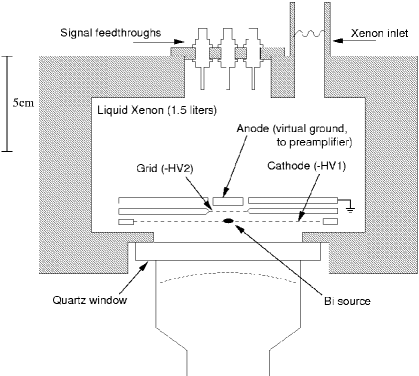
FIG. 1.: Schematic drawing of the liquid xenon detector. As described in the text, the chamber is cooled by immersion in a refrigerant bath. The bismuth source is in reality much smaller than indicated in the figure.

We have simultaneously studied both ionization and scintillation in LXe using a special geometry ionization chamber equipped with a VUV photomultiplier tube (PMT) capable of detecting the $\simeq 175$ nm scintillation light from the xenon. The chamber, shown in Figure 1, has a pancake geometry with a total volume of $\simeq 1.5$ liters. It is built out of ultra-high-vacuum compatible parts, so that it can be baked and treated with hot xenon before filling to obtain good LXe purity. The chamber is cooled by immersion in a bath of HFE7100 [8] that is in turn cooled by liquid nitrogen. The xenon is purified by an Oxysorb [9] cartridge during transfer from the storage cylinder to the chamber. Ionization is collected in a fiducial volume with radius $\simeq$ 10 mm and height $\simeq$ 6 mm defined by a small grid and a large cathode plane. The grid and cathode are made of an electroformed nickel mesh with 90% optical transparency. Drifted electrons are collected on a low-capacitance anode surrounded by a field defining ring held at the same ground potential. An electron transparency of 100% is obtained by maintaining the anode-to-grid field, ($E_{AG}$), double in value with respect to the drift field, ($E_{KG}$)[10], for all the measurements reported here. All data was collected at a LXe temperature of $169.2\pm 0.5$ K and pressure of $990^{+30}_{-50}$ Torr. The temperature gradients in the chamber were measured to be less than $\pm 0.2$ K.

The electron signal is detected by a low noise charge sensitive preamplifier[11] with a cold input FET placed on the feedthrough of the chamber. After subsequent amplification and filtering, the charge signal $f(t)$ is recorded on a transient digitizer and fit to a model assuming drift to the anode of a gaussian ionization distribution represented by the function

$$f(t)=A\left[1+erf\left(\frac{\Delta t}{C}\right)\right]e^{-\frac{t}{\tau}}+\alpha$$ (2)

where $\Delta t=t-t_{0}$ and the term $\alpha=De^{-\frac{t}{\tau}}+100+0.019t$ accounts for pile-up, ADC offset and a small integral non-linearity. We simultaneously fit for the amplitude $A$, the effective drift-time $t_{0}$, the rise-time parameter $C$, the pile-up offset $D$ and the integrator fall-time constant $\tau$. The fit fall-time is $\simeq 50~{}\mu$s for all the data, as expected. The parameter $C$ includes information about the multiplicity of the ionization event and its values range from 0.78 $\mu$s for a field of 4 kV/cm to 1.04 $\mu$s for 0.2 kV/cm. The decrease of this parameter with the increase of the electric field is consistent with the expected change in drift velocity.

The readout is calibrated in units of electron charge by injecting a signal into the input FET through a calibrated capacitor. The noise of the preamplifier was measured with a test signal and found to follow a gaussian distribution with width $\sigma_{N}=381e$.

The scintillation light is detected through the cathode grid by the 3-inch VUV PMT [12] with a solid angle that varies from 21.5% to 26% of $4\pi$ for signals produced in the region between cathode and grid active for ionization collection. The fraction of photoelectrons extracted from the PMT photocathode per scintillation photon produced in the LXe varies between 3.0% and 3.6% considering mesh and quartz window transparencies and photocathode quantum efficiency (22% including transparency of the PMT window). The PMT signal is read out using a 12 bit charge ADC calibrated by measuring the single-photon peak, which is well resolved from noise.

Data acquisition (DAQ) is triggered when there is a delayed coincidence between PMT and charge signals. The delay is required to account for the electron drift-time and varies with electric field. Once a coincidence is established, DAQ is inhibited until the event has been processed and the instruments cleared. About 25% of the collected data is removed off-line by analysis cuts that reject events that don’t fit model (2). These “bad events” are mostly due to multiple ionization deposits from Compton scattering, deposits at the edge of the ionization fiducial region, and cosmic ray background.

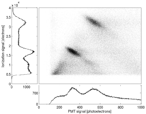
FIG. 2.: The two-dimensional scintillation and ionization spectra recorded at drift field $E_{KG}=4$kV/cm. The two “islands” with negative correlation coefficient correspond to the two $\gamma$ lines from the ²⁰⁷Bi source and their satellite internal conversion peaks. The axes are calibrated in terms of absolute numbers of elementary excitations (ionization electrons and photo-electrons in the PMT).

The LXe is excited by the 570 and 1064 keV $\gamma$’s (and their associated internal conversion electrons and X-rays) emitted by a ²⁰⁷Bi source. The source is prepared as a monoatomic layer electro-plated on a $\simeq 3\mu$m diameter carbon fiber that is then threaded through the cathode grid. The thin source minimizes the effects of self-shadowing of the scintillation light and is essential to obtain acceptable scintillation resolution. The data presented here were collected at drift fields $E_{KG}$ of 0.2kV/cm, 0.5kV/cm, 1kV/cm, 2kV/cm, and 4kV/cm.

A two-dimensional scatter plot of ionization versus scintillation signals obtained at 4 kV/cm is shown in Figure 2. The two peaks in the ionization channel can be fit to a gaussian function plus a first order polynomial function. The energy resolution obtained from the ionization data, once the electronics noise is subtracted in quadrature, is in good quantitative agreement with the results of other authors, as shown for the 570 keV peak in Figure 3.

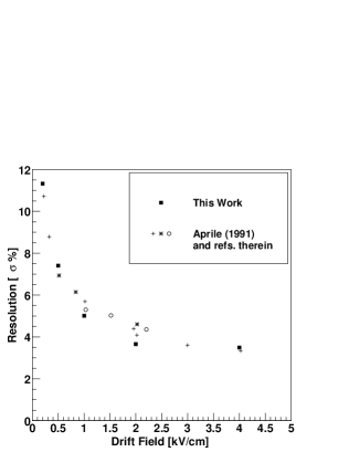
FIG. 3.: Ionization resolution for 570 keV $\gamma$s in LXe when fit to a one-dimensional gaussian. The black squares show the resolution observed by this experiment for different electric fields. The other symbols represent the resolutions observed with LXe ionization chambers by other authors [13], in good agreement with our data.

As shown in Figure 2, the scintillation spectrum has substantially poorer resolution and a larger continuum than the ionization spectrum. Differences between the two channels arise from the fact that the VUV photon acceptance depends somewhat upon the position of the energy deposited, as mentioned above, and from the different fiducial volumes. The resolution in the scintillation channel, as extracted by a fit with a gaussian plus a first degree polynomial, is $\sigma=(16.5\pm 2.5)\%$ at 570 keV, where the error refers to the range of values observed at different fields.

The observed ionization and scintillation spectra are qualitatively well reproduced in both peak positions and strengths by a detailed GEANT 4 [14] simulation which includes the processes of internal capture, X-ray and Auger electron emission. An empirical gaussian smearing is used to match the GEANT 4 output with the data. However, in the absence of a microscopic model for the production of scintillation photons in LXe, the simulation could not be used to quantitatively fit the two dimensional spectrum.

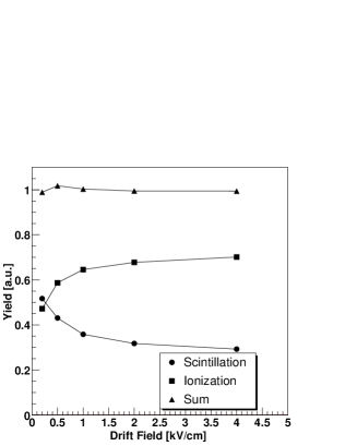
FIG. 4.: Macroscopic anti-correlation between scintillation light and ionization as a function of the electric field. Similar results have been obtained before by other workers.

Previous works [7] have reported evidence for what we call here “macroscopic” anti-correlation between scintillation light and ionization as a function of the electric field applied to the LXe. This effect, illustrated for our data in Figure 4, is thought to be due to the fact that scintillation occurs as ionization recombines. Different values of the electric field modify such recombination, changing the proportion between light and ionization but leaving their sum constant. The constancy of the sum is well reproduced by data, as shown, in our case, by Figure 4. We note that the absolute value of the sum does not directly correspond to the total energy deposited, as part of the energy is lost in other channels. We refer to this anti-correlation as “macroscopic” because is it an average behavior of the LXe and it is obtained by changing an external, macroscopic, parameter (the electric field).

In Figure 2, clear “microscopic” anti-correlation is evident in each of the two “islands” corresponding to the 570 keV and 1064 keV $\gamma$ lines. This effect, simply referred to as anti-correlation below, indicates that energy sharing between scintillation and ionization fluctuates event by event even though the sum of the two remains constant, in analogy with the macroscopic correlations described above. The microscopic nature of the anti-correlation may help in understanding the large Fano factor mentioned above. It also shows the way to dramatic improvements in the energy resolution of particle detectors, since the fluctuations clearly affect scintillation and ionization in opposite ways. Anti-correlations similar to the ones shown in Figure 2 are obtained at all fields and were not previously observed in LXe, although they were shown, without a detailed discussion, for heavy ions in liquid Argon, by Ref. [15].

The anti-correlation can be formally extracted from the data by fitting each of the peaks to a 2-dimensional gaussian distribution [16]

$$G(N_{e},N_{p})=He^{(\frac{-1}{2(1-\rho_{ep}^{2})}[\frac{\Delta N_{e}^{2}}{\sigma_{e}^{\prime 2}}+\frac{\Delta N_{p}^{2}}{\sigma_{p}^{2}}-\frac{2\rho_{ep}\Delta N_{e}\Delta N_{p}}{\sigma^{\prime}_{e}\sigma_{p}}])}$$ (3)

where $H=1/2\pi\sigma^{\prime}_{e}\sigma_{p}\sqrt{1-\rho_{ep}^{2}}$ is a normalization constant, $\rho_{ep}=V_{ep}/\sigma^{\prime}_{e}\sigma_{p}$ is the correlation coefficient between ionization and scintillation signals, $V_{ep}=\langle(N_{e}-\bar{N_{e}})(N_{p}-\bar{N_{p}})\rangle$ is the covariance, $\Delta N_{e}=N_{e}-\bar{N}_{e}$ and $\Delta N_{p}=N_{p}-\bar{N}_{p}$. While the instrumental noise on the scintillation channel is negligible and hence ignored, the variance for the ionization channel, $\sigma^{\prime 2}_{e}=\sigma^{2}_{e}+\sigma^{2}_{N}$, includes the term, $\sigma_{N}=381~{}e$, that accounts for the readout noise mentioned above. This is a relatively small correction (e.g. 12% at 4 kV/cm for the 570 keV peak). Unlike the one-dimensional fits used for ionization and scintillation data separately, the 2-dimensional fitting function does not include a background term. A two-step procedure is used to first find an elliptical region of full width $2.35\sigma$ around each of the two $\gamma$-ray peaks and then perform the final fit. The limited range of the fit suppresses the K-shell internal capture electrons and Compton scattering events. We found that the two-dimensional gaussian fits tend to produce larger variances with respect to the one-dimensional fits, providing a conservative estimate of the real resolutions.

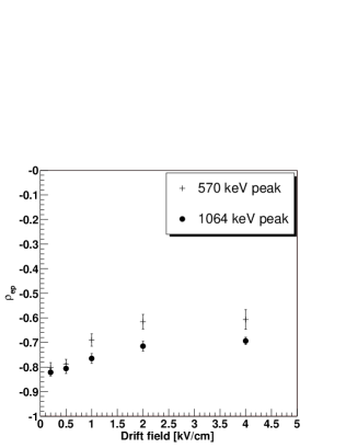
FIG. 5.: Correlation coefficients between ionization and scintillation signals obtained from the 2-dimensional fit discussed in the text. The two sets of points refer to the coefficients found for the 570 and the 1064 keV peaks. The errors shown are from systematics in the analysis, while statistical errors are negligible.

The correlation coefficients found by the fit are plotted in Figure 5 as a function of drift field. A clear anti-correlation exists at all fields for both the 570 keV and the 1064 keV lines. The errors shown in the Figure are systematic and are estimated as the full range of the variation of $\rho_{ep}$ when the different analysis cuts and fit intervals are changed. Statistical errors are negligible. The stability of the correlation with respect to different experimental circumstances (such as position in the chamber, size of the chamber and type of radiation) can be tested by repeating the fits for different subset of the data, each presenting a different range of effective drift-times, as derived from Eq. 2. The effective drift-time distribution, shown for 4 kV/cm in the inset of Figure 6, allows for the selection of events originating at different spatial positions along the drift field. The peak at large drift-times primarily corresponds to electrons that lose their energy and stop in the vicinity of the cathode plane where the source is. As shown in Figure 6 the correlation coefficient does not depend significantly on different effective drift times.

By diagonalizing the covariance matrix via a unitary rotation through angle $\theta=2\rho_{ep}\sigma_{e}\sigma_{p}/(\sigma_{e}^{2}-\sigma_{p}^{2})$, the correlated two-dimensional gaussian can be reduced to two uncorrelated gaussians with variances $\sigma_{min}^{2}$ and $\sigma_{max}^{2}$.[16] This rotation is mathematically equivalent to measuring the variances along the major and minor axes of the two-dimensional ellipses. Figure 7 shows the ionization resolutions from the 2-dimensional fit and the minimum resolutions in the frame rotated by $\theta$ for the 570 keV gamma ray peak at all drift fields.

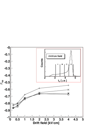
FIG. 6.: Correlation coefficient at all fields for different subset of events at a 4kV/cm field. The complete data set for the 570 keV region, is divided in four regions, according to their drift-times, as illustrated by the effective drift-time distribution in the inset. The peak to the right of this distribution is mostly due to electrons that stop near the source on the cathode. For each field the cuts defining different regions are set in such a way as to select equivalent populations of events. The magnitude of the correlation coefficients and their behavior as function of the electric field do not depend significantly upon the energy deposition location.

The resolution improvement observed when correlating the ionization and scintillation signals is significantly better than the uncorrelated addition of the two spectra, where $\sigma_{p+e}=(\sigma_{p}^{-2}+\sigma_{e}^{-2})^{-1/2}$. At 4 kV/cm $\sigma_{p+e}=3.7\%$. When using the correlated nature of the two channels the resolution $\sigma_{min}=3.0\%$, a factor of 1.24 improvement. The improvement is more dramatic at the 0.2 kV/cm field where the ratio is $9.7/5.4=1.8$. While we found that the absolute values of the resolution change somewhat for different fitting methods and at different stages of the iterative procedure, the improvement factor is very stable. We note here that the main results of this work are to show that a microscopic correlation exists and it can be consistently used to improve the resolution. The ultimate resolution will have to be measured at a later stage with a detector of larger volume, better VUV light collection and, possibly, a different source and it is expected to be even better than the resolution $\sigma_{min}$ reported in Figure 7.

While the nature of the large Fano factor in liquefied noble gases is still not well understood, the different models considered generally involve fluctuations in the density of the energy deposited [17]. Such fluctuations can arise from density variations in the medium or from the small number of delta electrons with energies between 1 and 30 keV that are produced by Rutherford scattering of atomic electrons in the liquid. When these electrons come to a stop they produce a dense cluster of electron-ion pairs whose recombination rate is relatively high. In both cases more recombination occurs where the ionization density is higher. Hence the statistics relevant for the fluctuations in the liquid is that of the (small) number of high ionization density regions (either the number of delta-electrons or the number of high density regions). In a sense, this would mean that the Fano factors computed in Eq. 1 are too small because the “wrong” $N$ is used.

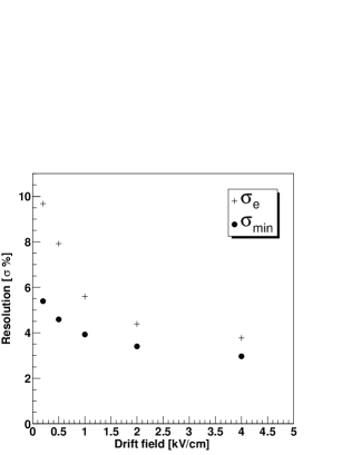
FIG. 7.: Resolutions for the ionization channel and for the small correlated combinations using a fit to a two-dimensional correlated gaussian. The data shown is for the 570 keV gamma ray peak.

As first suggested in Ref. [18] the recombination hypothesis above implies that the fluctuations of ionization and scintillation should be anti-correlated, since the high ionization-density regions which produce less free charge should emit a correspondingly larger amount of scintillation light. A linear combination of ionization and scintillation should therefore have smaller fluctuations than either alone. Note that since the Fano factors $F_{e}$ and $F_{p}$ are typically far in excess of their Poissonian values, the improvement should in principle be substantial and is not limited by the factor of $\sqrt{2}$ one would expect from the combination of two uncorrelated signals of equal resolution. The data presented here provides direct experimental evidence of this fluctuation and the associated recombination by observing a clear microscopic anti-correlation between ionization and scintillation. The correlation, $\rho_{ep}$, and the magnitude of the variances, $\sigma_{max}^{2}$ and $\sigma_{min}^{2}$, provide input to improve the model in terms of observables that are more directly related to the microscopic physics. It is interesting to note that from Figure 5 it appears that the magnitude of the correlation $\rho_{ep}$ decreases for increasing electric field (at least at low fields). This behavior is possibly connected to the dependence of the intensity of the recombination luminescence with the electric field, as expected in all the models discussed.

In conclusion, we have observed a clear microscopic anti-correlation between ionization and scintillation in liquid xenon. We have also measured the correlation coefficient between these two channels to be $-0.8<\rho_{ep}<-0.6$. This observation has two important consequences. First, it provides direct experimental evidence that recombination is a substantial source of the anomalously large Fano factors in the high density liquid state. Second, it provides a method for improving the resolution of liquefied noble gas calorimeters.

One of us (G.G.) is indebted to P. Picchi, F. Pietropaolo and T. Ypsilantis for early discussions on the subject, M. Moe for a careful reading of the manuscript and to R.G.H. Robertson for having stimulated the interest on this topic. This work was supported by US-DoE grant DE-FG03-90ER40569-A019 and by a Terman Fellowship of the Stanford University.

REFERENCES

- [1] T. Doke, in Experimental Techniques in High Energy Physics , T. Ferbel ed. (Addison Wesley, 1987).
- [2] U. Fano, Phys. Rev. 72 , 26 (1947).
- [3] N. Ishida, J. Kikuchi, T.Doke, and M. Kase, Phys. Rev. A 46 , 1676 (1992).
- [4] T. Doke, A. Hitachi, S. Kubota, A. Nakamoto, and T. Takahashi, Nucl. Instrum. Methods 134 , 353 (1976).
- [5] T. Doke and K. Masuda, Nucl. Instrum. Methods A 420, 62 (1999).
- [6] N. Schwentner, E.-E. Koch, and J. Jortner, in Electronic Excitations in Condensed Rare Gases Springer Tracts in Modern Physics, Vol. 107 (1985).
- [7] S. Kubota et al., Phys. Rev. B 17, 2762 (1978).
- [8] 3M refrigerant fluid, see http://products3.3m.com.
- [9] MG Industries, Specialty Gas Equipment, Allerton PA 18104.
- [10] O. Bunemann, T.E.Cranshaw, J.A.Harvey, Canadian J. of Research A 27, 191 (1949).
- [11] Amptek A250 with 2SK152 FET, see http://www.amptek.com.
- [12] Electron Tubes Model 9921Q.
- [13] E. Aprile et al., Nucl. Instrum. Methods A 302 , 177 (1991) and references therein.
- [14] S. Agostinelli et al. (GEANT4 Collaboration), “GEANT4: A simulation toolkit”, SLAC-PUB-9350.
- [15] E. Shibamura et al. Nuch. Instrum. and Methods A 260, 437 (1987).
- [16] K. Hagiwara et. al., Phys. Rev. D 66, 010001-1 (2002)
- [17] E. Shibamura et al., Jpn. J. Appl. Phys. 34, 1897 (1995) and references therein.
- [18] J. Seguinot, G. Passardi, J. Tischhauser, and T. Ypsilantis, Nucl. Instrum. Methods A 323 , 583 (1992).