Key words: Underground muons, Neutron flux, Neutron production by muons, Dark matter experiments, Neutron background

PACS: 96.40.Tv, 25.40.Sc, 25.30.Mr, 28.20.-v

Corresponding author: V. A. Kudryavtsev, Department of Physics and Astronomy, University of Sheffield, Hicks Building, Hounsfield Rd., Sheffield S3 7RH, UK

Tel: +44 (0)114 2224531;                   Fax: +44 (0)114 2728079;

E-mail: v.kudryavtsev@sheffield.ac.uk

1. Introduction

Existing and planned dark matter searches and neutrino detection experiments require very sensitive equipment and sophisticated data acquisition capable of tagging events from the source and discriminating them from all kinds of background. Some background, however, is undistinguishable from the expected signal events. As an example of this we can mention neutron background in experiments searching for dark matter particles in the form of Weakly Interacting Massive Particles (WIMPs), also known as neutralinos, the lightest supersymmetric particle in SUSY models. WIMPs are expected to interact with ordinary matter in detectors to produce nuclear recoils, which can be detected through ionisation, scintillation or phonons. Identical events can be induced by neutrons. Thus, only suppression of any background neutron flux by passive or active shielding will allow experiments to reach sufficiently high sensitivity to neutralinos. Designing shielding for such detectors requires simulation of neutron fluxes from various sources.

Neutrons underground arise from two sources: i) local radioactivity, and ii) cosmic-ray muons. Neutrons associated with local radioactivity are produced mainly via ($\alpha$, n) reactions, initiated by $\alpha$-particles from U/Th traces in the rock and detector elements. Neutrons from spontaneous fission of ²³⁸U contribute also to the flux at low energies. The neutron yield from cosmic-ray muons depends strongly on the depth of the underground laboratory. It is obvious that suppression of the muon flux by a large thickness of rock will also reduce the neutron yield. The dependence, however, is not linear.

In general, at large depth underground the neutron production rate due to muons is about 3 orders of magnitude less than that of neutrons arising from local radioactivity. (Note that this figure depends strongly on the depth and U/Th contamination). The muon-induced neutron flux can be, however, important for experiments intending to reach high sensitivity to WIMPs or to low-energy neutrino fluxes. There are several reasons for this: 1) the energy spectrum of muon-induced neutrons is hard, extending to GeV energies, and fast neutrons can travel far from the associated muon track, reaching a detector from large distances; 2) fast neutrons transfer larger energies to nuclear recoils making them visible in dark matter detectors, while many recoils from $\alpha$-induced neutrons fall below detector energy thresholds; 3) a detector can be protected against neutrons from the rock activity by hydrogen-rich material, possibly with addition of thermal neutron absorber; such a material, however, will be a target for cosmic-ray muons and will not protect against muon-induced neutrons. The only way to reduce this flux is to add an active veto, rejecting all events associated with passing muons.

In this paper we discuss neutron production by muons at large depth underground. There are several reactions which lead to neutron appearance. The main processes are: a) negative muon capture; this process occurs with stopping muons and plays a significant role only at shallow depth; b) muon-induced spallation reactions; c) neutron production by hadrons (and photons) in muon-induced (via photonuclear interaction) hadronic cascades; d) neutron production by photons in electromagnetic cascades initiated by muons.

The muon-induced neutron case was first discussed by Zatsepin and Ryazhskaya [1] and its importance for large proton decay and neutrino experiments was studied [2]. Some results are summarised in Ref. [3]. Several measurements of the neutron flux underground have been performed [4, 5, 6, 7, 8, 9]. However, no precise three-dimensional simulation of neutron production has been done for most experiments. Recently accurate versions of Monte Carlo codes FLUKA [10] and GEANT4 [11], designed for particle transport over a wide energy range, have become available. They are capable of simulating neutron production by muons, hadrons and photons, as well as neutron transport and interactions in the detector volume. Simulations of neutron production by muons with FLUKA have been performed by Battistoni et al. [12] and Wang et al. [13]. The authors of Ref. [13] studied neutron production by muons in scintillator and compared the results with existing data. Recently extensive neutron background studies have been initiated by the joint EDELWEISS/CRESST team of dark matter experiments at Gran Sasso and Modane [14].

In this work we have used the FLUKA code for neutron production and transport. We have calculated the neutron production rate in scintillator for several muon energies and have compared our results with those from Ref. [13] and with experimental data. We have studied the neutron production rate as a function of the atomic weight of the target material. We have calculated the neutron flux as a function of distance from muon tracks, which is very important for designing muon veto systems, and we have compared the result with available data. Finally, we have used MUSIC [15, 16, 17] to simulate the muon energy spectrum underground and we have calculated neutron production from the muon spectrum.

The work has been done as a part of a programme of neutron background studies for the dark matter experiments at Boulby mine (North Yorkshire, UK) (see Ref. [18] for a review of dark matter searches at Boulby). We hope that other experiments having similar background problems will benefit from this work too.

The paper is organised in the following way. Muon fluxes, energy spectra and their uncertainties are discussed in Section 2. Simulations of muon-induced neutrons are presented in Section 3. The conclusions are given in Section 4.

2. Muon flux and energy spectrum underground

Knowledge of the muon flux is clearly important for calculations of the neutron flux or counting rate – it provides the absolute normalisation. The muon energy spectrum at a given experimental site also affects the neutron production rate. Thus precise knowledge of the muon spectrum and absolute normalisation is crucial for neutron flux simulations.

To calculate the muon fluxes and energy spectra at large depths underground, we used here parameterisation of the surface muon spectrum propagated through the rock using the MUSIC code. The calculation was performed in the following way. First, muons with various energies at the surface were transported using MUSIC [15, 16] down to 15 km w.e. of rock underground and their energy distributions at various depths stored on disk. For a set of muon energies at sea level, and for a set of different depths underground, the muon energy distributions were obtained in the form $P(E_{\mu},X,E_{\mu 0})$ – the probability for a muon with energy $E_{\mu 0}$ at the surface to have energy $E_{\mu}$ at depth $X$. If no muon with a certain energy survives, then the probability to reach the depth will be equal to 0. Muons were propagated in several types of rock, including standard rock, Gran Sasso rock and Boulby rock.

Special codes were used to calculate differential and integral muon intensities at the various depths (code SIAM) and to simulate muon spectra and angular distributions (code MUSUN). The codes had previously been used to simulate single atmospheric muons under water [17]. A brief description of the codes [19] is given below.

To calculate the differential muon intensity underground the following equation was used:

$$I_{\mu}(E_{\mu},X,\cos\theta)=\int_{0}^{\infty}P(E_{\mu},X,E_{\mu 0}){{dI_{\mu 0}(E_{\mu 0},\cos\theta^{\star})}\over{dE_{\mu 0}}}dE_{\mu 0}$$ (1)

where ${{dI_{\mu 0}(E_{\mu 0},\cos\theta^{\star})}\over{dE_{\mu 0}}}$ is the muon spectrum at sea level at zenith angle $\theta^{\star}$ (the zenith angle at the surface, $\theta^{\star}$, was calculated from that underground, $\theta$, taking into account the curvature of the Earth).

The energy spectrum at sea level was taken either according to the parameterisation proposed by Gaisser [20] (modified for large zenith angles [21]) or following the best fit to the ‘depth – vertical muon intensity’ relation measured by the LVD experiment [21]. The first parameterisation [20] has a power index for the primary all-nucleon spectrum of 2.70, while the second one [21] uses the index 2.77 with normalisation to the absolute flux measured by LVD. The difference between the results obtained with these two spectra shows a possible spread in the muon energy spectra at the surface and, hence, in muon intensities underground.

The ratio of prompt muons (from charmed particle decay) to pions was chosen as $10^{-4}$, which was well below an upper limit set by the LVD experiment [22]. Note, however, that the prompt muon flux does not significantly affect muon intensities even at large depths.

To calculate the integral muon intensity, an integration of $I_{\mu}(E_{\mu},X,\cos\theta)$ over $dE_{\mu}$ was carried out. An additional integration over $\cos\theta$ defined the global intensity for a spherical detector.

The muon energy spectrum, fraction of prompt muons, type of rock and depth can be chosen in the SIAM and MUSUN codes.

The muon intensities, calculated with SIAM for two types of rock, two parameterisations of muon energy spectrum at the surface and at several depths are given in Table 1. Our present calculations agree well with previous results obtained with MUSIC [15]. Note that only a few modifications (including more recent cross-sections) have been implemented in the code [16] since the first version was published [15].

The absolute muon flux (intensity) underground depends on the surface relief, which should be taken into account for any particular experiment. For a complex mountain profile, as for the Gran Sasso and Modane underground laboratories, it is difficult to give predictions of the muon flux without precise knowledge of the slant depth distribution. For a flat surface above a detector the calculations are straightforward. We present here the results for vertical and global (integrated over solid angle for spherical detector) muon intensities under a flat surface for standard rock ($<Z>=11,<A>=22$). We used parameterisation of the muon spectrum at sea level according to a best fit to the ‘depth – vertical intensity’ relation measured by the LVD experiment at Gran Sasso. Note that the LVD results agree well with those of the MACRO experiment [23].

The ratio of global intensity (column 3) to the vertical one (column 2) gives an average solid angle for a particular depth under a flat surface. It decreases from about 2 sr down to about 0.5 sr for depths from 0.5 km w.e. down to 10 km w.e., being about 1 sr at 3-4 km w.e., at which many experiments are located.

Intensities calculated with Gaisser’s parameterisation of muons at the surface [20] (column 4) are lower by 20% at small depths and higher by 15% at large depths compared to the LVD parameterisation (column 3). This is due to differences in the power index of the muon spectrum and absolute normalisation. Gaisser’s parameterisation describes reasonably well the muon data at low energies (below 1 TeV), while the LVD data provide a good parameterisation for the muon spectrum above 1.5-2 TeV (for depths more than 3 km w. e.).

The muon intensities in Boulby rock (column 5), which has slightly higher mean values of atomic number and weight ($<Z>\approx 11.7,<A>\approx 23.6$), are smaller than in standard rock (column 3) due to the larger muon energy losses, which are proportional to $Z^{2}/A$. The difference, however, does not exceed 5% at depths smaller than 2 km w.e., where the ionisation energy loss (proportional to $Z/A$) dominates. At 3 km w.e. the difference is about 8%, which gives an uncertainty in $<Z>$ and $<A>$ of about 2-3% acceptable from the point of view of the accuracy required for muon and neutron flux simulations here.

The muon energy spectrum underground is also important for neutron flux simulations, since neutron production rates increase with muon energy. While the absolute muon flux underground can be measured to check simulations, the muon energy spectrum is hard to determine experimentally. We have to rely on simulations. The mean muon energy is a parameter, which characterises well the muon energy spectrum. Table 2 shows the calculations of mean muon energies underground.

An important conclusion, which can be derived from comparison of the mean muon energies for global fluxes, is that their spread is much smaller than that for the fluxes themselves. The mean muon energies are very similar for different types of rock at small depths and differ by no more than 5% at large depths. The two different parameterisations of the muon spectrum at sea level result in the $\approx 5\%$ difference in mean energy. For a fixed slant depth the mean energy for inclined muon directions ($60^{\circ}$ in our simulations) is very close to that at vertical. The increase in mean energy for the global flux compared to the vertical flux is due to the increase of slant depth with zenith angle. With increasing depth, the effective solid angle decreases (see Table 1 and the discussion above), and the mean muon energy for global flux becomes closer to that at vertical.

It is interesting to estimate uncertainties in the muon flux and mean energy for a fixed depth due to uncertainties in depth, density, rock composition and parameterisation of the muon spectrum at the surface. Depth and rock density have a similar effect on the muon flux, since the intensity depends on their product – column density expressed in metres of water equivalent or hg/cm². Changing the column density (either depth or density) by 2% results in a 10% change in muon flux at 3 km w.e. and has no effect on the muon energy spectrum. An increase of $<Z>$ and $<A>$ by about 7% (changing from standard to Boulby rock, for example) without changing the density gives an 8% decrease in the flux and a 3% increase in the mean energy at 3 km w.e. Finally, 7% uncertainty in the flux and 4% uncertainty in the mean energy at 3 km w.e. may arise from the difference in parameterisations of the muon spectrum at sea level. Note, however, that the LVD experiment provides direct measurements of muon intensities at 3 km w.e. and below, which were used to derive the parameterisation for muon flux at sea level. So, unless the experimental site is at shallow depth, the LVD parameterisation is the preferred option.

Two measurements of mean muon energy underground carried out with the NUSEX [24] ($<E_{\mu}>=346\pm 14\pm 17$ GeV for vertical muons at 5 km w.e. in standard rock) and MACRO [25] ($<E_{\mu}>=270\pm 3\pm 18$ GeV for single muons at 3.0-6.5 km w.e. in standard rock) detectors are in reasonable agreement with our simulations (see Table 2). Note that the experimental errors quoted by the authors [24, 25] are larger than the possible systematic uncertainty of the simulations with a particular code. There is a large spread of muon intensities and mean energies as calculated with a number of muon propagation codes (see, for example discussion in Ref. [24]). Note, however, that in our simulations we used the results obtained with the MUSIC code, which was tested against experimental underground muon data [21, 22, 26].

3. Simulations of muon-induced neutrons

As can be seen from Tables 1 and 2 and discussion above, the uncertainty in absolute muon flux is larger than that of the muon energy spectrum underground (mean energy). This conclusion is encouraging because the absolute flux can be measured directly, while it is difficult to determine the mean muon energy from experiment. Thus, the uncertainty in neutron flux is almost directly proportional to that in the muon flux.

Neither code provides an absolute accuracy in the neutron simulation. There is always an uncertainty related to our knowledge of the neutron production mechanism and to the choice of the model for its description. In our opinion the FLUKA [10] and GEANT4 [11] codes are the best suited for this job. We simulated neutron production by muons with FLUKA [10]. The models of photoproduction and hadronic interactions, used in FLUKA, are described in the Refs. [10, 13].

It is widely accepted (see, for example, Ref. [3, 6, 13] and references therein) that the neutron production at a certain depth can be approximated by assuming that neutrons are produced by muons, all having mean energy corresponding to this depth. Keeping this in mind we started with the simulations of neutron production in scintillator (C₁₀H₂₀) as a function of muon energy in order to compare the results with available experimental data and previous simulations with FLUKA [13].

As many neutrons are produced in large cascades initiated by muons, the equilibrium between neutron and muon fluxes (when the ratio of neutron to muon fluxes is constant) begins only when a muon has crossed a certain thickness of a medium. This is because cascades need some depth to develop and produce neutrons. So, the thickness of medium was chosen large enough (of the order of 4000-5000 g/cm²) for such an equilibrium to take place, and only neutrons in a reduced layer of a medium (where the equilibrium is in place) were counted.

Large thicknesses of material produce, however, another effect: the muon energy can be reduced compared to the initial value due to interactions with matter. This is particularly important for low energies. We checked carefully that the neutron flux in our simulations did not decrease with the thickness of a medium crossed by muons. Where a reduction in flux could not be avoided (for low muon energies), the appropriate correction of the order of a few percent was applied.

The FLUKA code returned the number of neutrons in various layers in a medium and neutron spectra in various regions and at the boundaries between regions. Some neutrons, however, are counted twice (see also the discussion in Ref. [13]). This happens when a neutron produces a star. Then, the scattered neutron is counted also as a secondary neutron (with different energy). To avoid double counting, the number of stars produced by neutrons was subtracted from the total number of neutrons.

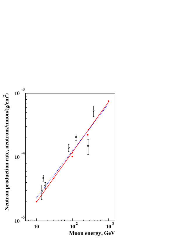
Figure 1: Average number of neutrons produced by a muon per unit path length (1 g/cm²) in scintillator as a function of muon energy. Our results are shown by filled circles. The parameterisation with Eq. (1) is shown as a solid line. The parameterisation found in Ref. [13] is plotted by a dashed line. The measurements shown are as follows (in order of increasing energy): 20 m w.e. (minimal depth) [9, 8], 25 m w.e. [4], 32 m w.e. [8], 316 m w.e. [4], 570 m w.e. [5], 3000 m w.e. [7], 5200 m w.e. [6]. Filled squares show the number of neutrons, produced in scintillator by muons with a real spectrum for depths of 0.55 km w.e. and 3 km w.e. in Boulby rock (mean energies 98 and 264 GeV, respectively).

The average number of neutrons produced by a muon per unit path length (1 g/cm²) in scintillator is presented in Figure 1 as a function of muon energy. Our results (filled circles) have been fitted to a function:

$$R_{n}=a\times E^{\alpha}$$ (2)

where $a=(3.20\pm 0.10)\times 10^{-6}$ and $\alpha=0.79\pm 0.01$. The agreement with simulations by Wang et al. [13] (dashed line shows the fit) is pretty good. Note that Wang et al. [13] performed the simulations in scintillator with a slightly different fraction of carbon and hydrogen atoms (C₁₀H₂₂), but this should not significantly affect the neutron production. The small difference between the simulation results can be attributed to a number of corrections described above and in Ref. [13].

Also shown in Figure 1 are the measurements of neutron production by several experiments. In the experiments neutrons were produced by muons with a certain spectrum. Here we have plotted their results as a function of mean muon energy underground. For experiments at large depths (more than 400 m w.e.) we used the mean muon energy calculated by the authors. Our simulations, however, predict smaller mean muon energies at these depths with the exception of the LVD result (270 GeV). (Note that, to evaluate mean muon energy for the LVD experiment, the same MUSIC propagation code and LVD depth–intensity curve were used by the authors [21]). For shallow depths we used estimates of the mean muon energies from Ref. [13].

All measurements, except those of LVD, show higher neutron production rate than simulations with FLUKA. Similar conclusion was reached in Ref. [13]. If the data points were shifted to smaller muon energies, then the disagreement would become even more prominent. So, an error in the calculation of mean muon energy cannot explain the difference.

Another possible explanation could be the difference in neutron production between muons with fixed mean energy and muons with a real spectrum underground. This was checked by simulating neutron production in scintillator by muons with a real spectrum for depths of 0.55 km w.e. and 3 km w.e. in Boulby rock (mean energies 98 and 264 GeV, respectively; filled squares in Figure 1). In both cases a smaller neutron production rate in scintillator was found. The difference is of the order of (10-15)% for large range of depths (0.5 – 3 km w.e.) and mean muon energies (100 – 300 GeV). (Note that a few percent decrease in the neutron production is expected due to the attenuation of the muon flux with realistic spectrum with mean energy of 280 GeV when muons are crossing a few tens of m w.e.). A similar difference was found also for neutron production in NaCl salt. For marl rock (mainly CaCO₃), however, the difference is not significant, the neutron production rate for mean muon energy of 280 GeV being about $4.0\times 10^{-4}$ neutrons/muon/(g/cm³). Neutron production rate in lead by muons with an energy spectrum with mean energy of 280 GeV (as at 3.2 km w.e. depth in standard rock) is 10% higher than that by muons with a fixed energy of 280 GeV. The difference between neutron production by a muon spectrum and by muons with fixed mean energy and the dependence of this effect on the target material emphasise the importance of the simulations with realistic input data, such as muon energy spectrum and target composition. The smaller neutron production rate in scintillator calculated with a real muon spectrum makes agreement between LVD data and simulations better, while other experimental results are less consistent with predictions.

The difference between LSD and LVD measurements (385 GeV and 270 GeV, respectively) represents a real puzzle. Although performed at different depths, the experiments used a similar modular structure, similar liquid scintillator counters and similar analysis techniques. Clearly, better study of systematic effects is needed.

In our simulations with fixed muon energies we did not observe any significant difference in neutron production by positive and negative muons with energies above 10 GeV, which proved the absence of muon capture. Only the real muon spectrum at small depth could, in principle, produce a significant number of stopping muons and, consequently, neutrons through negative muon capture. At large depth, where the number of stopping muons is negligible, negative muon capture does not contribute much to neutron production.

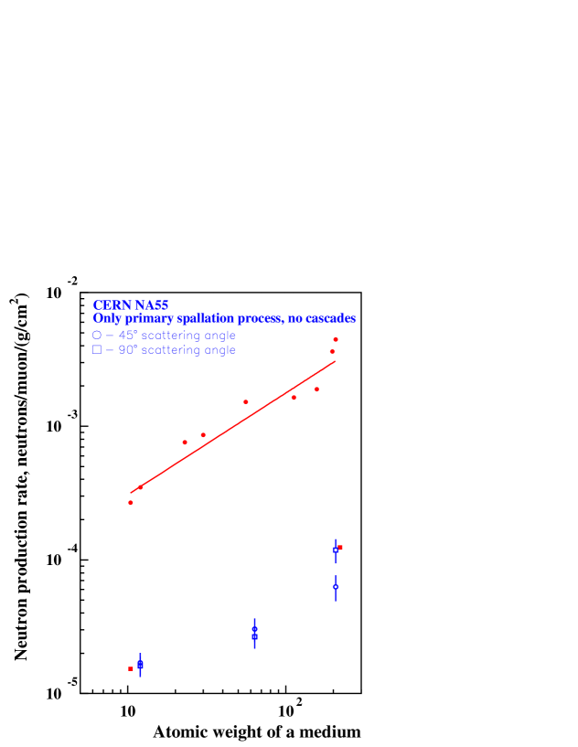
Figure 2: Dependence of neutron rate on the atomic weight of material. Materials and compounds used in the simulations and presented in the figure by filled circles are (in order of increasing atomic weight): C₁₀H₂₀ ($<$$A$$>$=10.4), C ($<$$A$$>$=12.0), Na ($<$$A$$>$=23.0), NaCl ($<$$A$$>$=30.0), Fe ($<$$A$$>$=55.9), Cd ($<$$A$$>$=112.4), Gd ($<$$A$$>$=157.3), Au ($<$$A$$>$=197.0), and Pb ($<$$A$$>$=207.2). A simple parameterisation by a power-law is given by the solid line. Also shown are the measurements of neutron rate by NA55 at CERN in three thin targets at two neutron scattering angles (open circles and open squares) (see text for details). These are normalised at small atomic weight (carbon) to our simulations with FLUKA for the muon spallation only (filled squares). For the muon spallation our result for lead is artificially shifted to A=220 to avoid the overlaping with one of the CERN points.

We studied also the dependence of neutron rate on the atomic weight of material. The neutron rate was obtained with 280 GeV muon flux in several materials and compounds and is shown in Figure 2 by filled circles. The errors of the simulations do not exceed 5% and are comparable to the size of the circles on the figure. It is obvious that on average the neutron rate increases with the atomic weight of material, but no exact parameterisation was found which would explain the behaviour for all elements and/or compounds. The general trend can be fitted by a simple power-law form (solid line in Figure 2):

$$R_{n}=b\times A^{\beta}$$ (3)

where $b=(5.33\pm 0.17)\times 10^{-5}$, $A$ is the atomic weight (or mean atomic weight in the case of a compound) and $\beta=0.76\pm 0.01$. It is clear from the figure, however, that the points on Figure 2 are largely spread around the line. We compared our results with measurements performed in the NA55 experiment at CERN with a 190 GeV muon beam [27]. The neutron production was measured in thin targets at several neutron scattering angles, so direct comparison with our simulations is difficult. The use of thin targets allowed the measurement of neutron production in the first muon interaction only (without accounting for neutrons produced in cascades) [27]. We calculated neutron production in the first muon interaction in scintillator and lead and plotted it in Figure 2 (filled squares) together with the measurements [27] at two scattering angles (open circles and open squares). Since the measured values refer to particular scattering angles, we normalised them to our results at small atomic weight (carbon). The measured behaviour of the neutron rate with atomic weight agrees well with FLUKA predictions.

The processes contributing to neutron flux were studied in Ref. [13] for a liquid scintillator as a target. We performed a similar investigation for scintillator and extended it to heavy targets. We subdivided the neutron production by muons into three main processes: i) direct muon-induced spallation (first muon interaction), ii) muon-induced hadronic cascades, and iii) muon-induced electromagnetic cascades. We neglected negative muon capture, which contributes only at small depths or small muon energies. We found that in scintillator at a muon energy of 280 GeV, 75% of neutrons are produced in hadronic cascades, 20% in electromagnetic cascades, and 5% in muon-induced spallation. The last number will be increased up to 9% if secondary neutrons produced in collisions of neutrons from muon spallation with nuclei are counted here and not in the hadronic cascades. For 10 GeV muons the contribution from hadronic cascades drops to 38%, while electromagnetic cascades contribute to 35% of neutrons, and muon spallation is responsible for 27% of neutrons (36% if secondary neutrons are counted here). This is due to a smaller muon photoproduction cross-section at these energies. (Note that the error in the calculations at low energies is quite large, about 3-5%, due to the small number of neutrons produced and large corrections involved).

For a heavy target (e.g. lead) the contribution from electromagnetic cascades becomes more important (42% for 280 GeV muons) because the cross-section of electromagnetic muon interactions is proportional to $Z^{2}/A$. Hadronic cascades give about 55% of neutrons for 280 GeV muons and muon-induced spallation is responsible for the remaining 3% (10% if secondary neutrons from neutron-nucleus collisions are counted here and not in hadronic cascades).

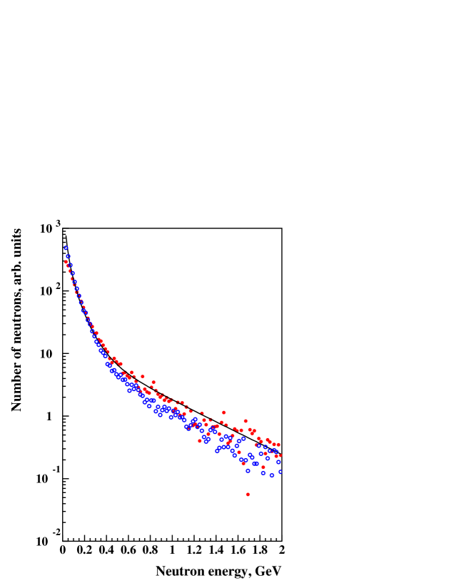
Figure 3: Neutron energy spectrum in scintillator (filled circles) and NaCl (open circles) obtained with muon spectrum at about 3 km w.e. underground. Parameterisation proposed in Ref. [13] for scintillator for muon energy 280 GeV is shown by the solid line, arbitrarily normalised to our simulations to reach visual agreement. Arbitrary units are used for all spectra, the normalisation being provided by the total neutron production rate (see Figures 1 and 2).

The neutron energy spectrum was calculated for various targets. Figure 3 shows the spectrum obtained for scintillator and NaCl together with parameterisation proposed for scintillator in Ref. [13]. In our simulations the real muon spectrum at about 3 km w. e. underground was used. The parameterisation for scintillator [13] was obtained for 280 GeV muons, which is close to the mean energy of the muon spectrum used in the present work. Two conclusions can be derived from figure 3: i) the parameterisation proposed in Ref. [13] agrees with our simulations only at neutron energies higher than 50 MeV; this may be partly due to the fact that in our simulations all muon energies contribute to the neutron production, ii) the neutron energy spectrum becomes softer with increase of $<A>$, although the total neutron production rate increases (see Figure 2).

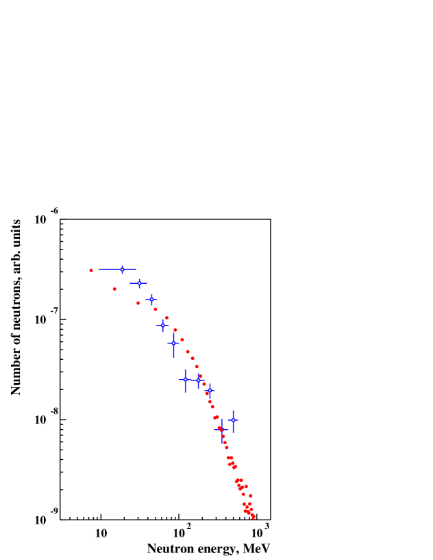
Figure 4: Neutron energy spectrum in scintillator (filled circles) in comparison with the LVD data [7]. LVD data are normalised to the calculated spectrum to reach better visual agreement. The absolute normalisation is provided by the total neutron production rate (see Figure 1).

Figure 4 shows the neutron energy spectrum in scintillator (filled circles) in comparison with the LVD data (open circles with error bars) [7]. LVD reported in fact the number of events as a function of energy deposition, which is not equal to the neutron energy. The major difference comes probably from the quenching of protons in the scintillator, assuming that the energy deposition is due to the energy loss of protons from elastically scattered neutrons. The LVD data points, presented in Figure 4 have been corrected for the quenching factor typical for organic liquid scintillators [28]. The agreement is reasonably good taking into account large uncertainties in the conversion of visible energy into neutron energy.

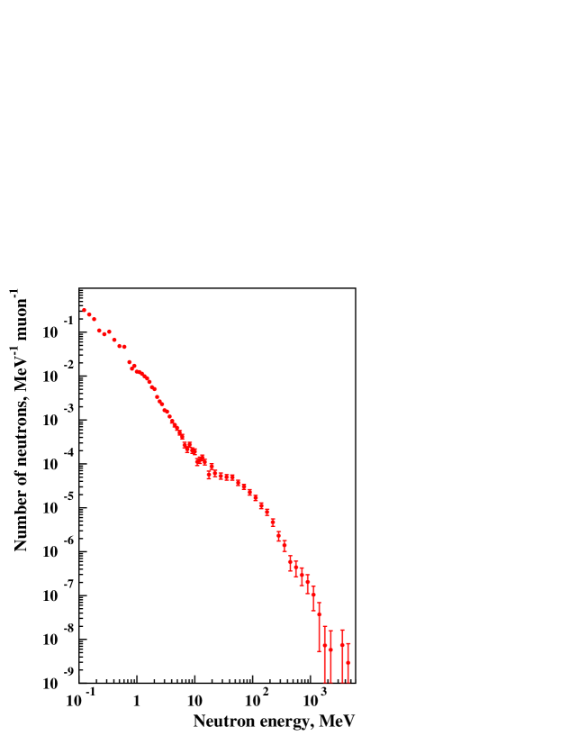
Figure 5: Neutron energy spectrum at the boundary between salt and cavern.

The next step is calculation of the energy spectrum of neutrons coming from the rock into the laboratory hall or cavern. We have carried out such a simulation for salt with the real muon energy spectrum for Boulby. The volume of the salt region was taken as $20\times 20\times 20$ m³, with the cavern for the detector of size $6\times 6\times 5$ m³. The top of the cavern was placed at a depth of 10 m from the top of the salt region. The neutrons in the simulations did not stop in the cavern but were propagated to the opposite wall where they could be scattered back into the cavern and could be counted for the second time. Figure 5 shows the simulated neutron energy spectrum at the salt/cavern boundary. To obtain the neutron flux in units MeV^-1 cm^-2 s^-1 the differential spectrum plotted on Figure 5 has to be multiplied by the muon flux (see Table 1). The total number of neutrons entering the cavern is about $5.8\times 10^{-10}$ cm^-2 s^-1 above 1 MeV at 3 km w.e. in Boulby rock. The flux on an actual detector can be different from the flux on the boundary salt/cavern due to the interactions of neutrons in the detector itself.

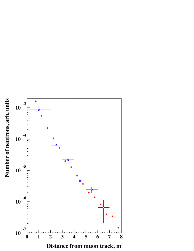
Figure 6: Simulated neutron rate as a function of distance from the muon track in scintillator (filled circles) in comparison with the LVD data [7]. LVD data are normalised to the calculated distribution to get better visual agreement. The absolute normalisation is provided by the total neutron production rate (see Figure 1).

One of the most important features of the muon-induced neutron background relevant for dark matter and neutrino experiments is the lateral distribution of neutrons, i.e. the number of neutrons as a function of distance from muon track. Such a distribution gives the probability that a neutron can mimic an expected signal at various distances from a muon track, if neither muon or neutron are detected by an active veto. Figure 6 shows the simulated lateral distribution of neutrons in scintillator in comparison with the LVD data [7]. The agreement between them is very good, although LVD is not a detector with a single uniform medium, but has a modular structure with gaps between modules.

4. Conclusions

We have discussed muon-induced neutron background relevant to dark matter and neutrino experiments. We have presented calculations of muon fluxes and energy spectra at various depths underground and estimated their uncertainties. Neutron production by cosmic-ray muons was simulated for various muon energies and various materials. We found reasonably good agreement with the recent experimental data of the LVD experiment [7]. The MUSIC code with associated packages (SIAM and MUSUN), together with FLUKA, provide a good tool for simulating muon fluxes and muon-induced neutron background at various depths underground. Our simulation is the starting point of a three-dimensional Monte Carlo to study the neutron background for any detector.

5. Acknowledgments

The authors wish to thank the members of the UK Dark Matter Collaboration and the Boulby Dark Matter Collaboration for valuable discussions. We are grateful, in particular, to Prof. P. F. Smith, Dr. N. J. T. Smith, Dr. J. D. Lewin and Prof. G. Gerbier, for useful comments. We thank also Dr. I. Dawson for his help to run and understand FLUKA.

Table 1: Muon intensities at various depths underground for standard and Boulby rock and two parameterisations of muon spectrum at the surface. Column 1 – depth in kilometres of water equivalent, km w.e.; column 2 – vertical muon intensity in standard rock in cm^-2 s^-1 sr^-1 with parameterisation of the muon spectrum at sea level according to the best fit to LVD data [21]; column 3 – global intensity (integrated over solid angle for a spherical detector) in standard rock (cm^-2 s^-1) for a flat surface with LVD parameterisation of the muon spectrum; column 4 – global intensity in standard rock (cm^-2 s^-1) for a flat surface with Gaisser’s parameterisation of the muon spectrum at sea level [20]; column 5 – global intensity for Boulby rock ($<Z>=11.7,<A>=23.6$) with LVD parameterisation of the muon spectrum.

$X$, km w.e.	$I_{\mu}^{vert}$, s.r., LVD	$I_{\mu}$, s.r., LVD	$I_{\mu}$, s.r., Gaisser	$I_{\mu}$, Boulby, LVD
0.5	$1.08\times 10^{-5}$	$2.12\times 10^{-5}$	$1.70\times 10^{-5}$	$2.12\times 10^{-5}$
1.0	$1.48\times 10^{-6}$	$2.60\times 10^{-6}$	$2.20\times 10^{-6}$	$2.57\times 10^{-6}$
2.0	$1.39\times 10^{-7}$	$2.01\times 10^{-7}$	$1.81\times 10^{-7}$	$1.93\times 10^{-7}$
3.0	$2.59\times 10^{-8}$	$3.15\times 10^{-8}$	$2.94\times 10^{-8}$	$2.91\times 10^{-8}$
4.0	$6.27\times 10^{-9}$	$6.54\times 10^{-9}$	$6.33\times 10^{-9}$	$5.84\times 10^{-9}$
5.0	$1.74\times 10^{-9}$	$1.58\times 10^{-9}$	$1.58\times 10^{-9}$	$1.36\times 10^{-9}$
6.0	$5.23\times 10^{-10}$	$4.21\times 10^{-10}$	$4.30\times 10^{-10}$	$3.48\times 10^{-10}$
7.0	$1.65\times 10^{-10}$	$1.18\times 10^{-10}$	$1.24\times 10^{-10}$	$9.41\times 10^{-11}$
8.0	$5.38\times 10^{-11}$	$3.47\times 10^{-11}$	$3.73\times 10^{-11}$	$2.65\times 10^{-11}$
9.0	$1.79\times 10^{-11}$	$1.05\times 10^{-11}$	$1.15\times 10^{-11}$	$7.69\times 10^{-12}$
10.0	$6.06\times 10^{-12}$	$3.25\times 10^{-12}$	$3.65\times 10^{-12}$	$2.27\times 10^{-12}$

Table 2: Mean muon energies in GeV at various depths underground for standard and Boulby rock and two parameterisations of the muon spectrum at the surface. Column 1 – depth in kilometres of water equivalent, km w.e.; column 2 – mean muon energy for vertical muon flux in standard rock with parameterisation of the muon spectrum at sea level according to the best fit to the LVD data [21]; column 3 – mean muon energy for global muon flux in standard rock for a flat surface with LVD parameterisation of the muon spectrum; column 4 – mean muon energy for global muon flux in standard rock for a flat surface with Gaisser’s parameterisation of the muon spectrum at sea level [20]; column 5 – mean muon energy for global muon flux for Boulby rock with LVD parameterisation of the muon spectrum; column 6 – mean muon energy for muon flux at 60^o in standard rock with LVD parameterisation of the muon spectrum (for this column the values in column 1 show the slant depth instead of vertical depth).

$X$	$<E_{\mu}^{vert}>$	$<E_{\mu}>$	$<E_{\mu}>$	$<E_{\mu}>$	$<E_{\mu}^{60}>$
km w.e.	s.r., LVD	s.r., LVD	s.r., Gaisser	Boulby, LVD	s.r., LVD
0.5	68	92	97	91	74
1.0	120	150	157	147	127
2.0	197	226	236	220	205
3.0	249	273	285	264	256
4.0	286	304	316	293	292
5.0	312	324	337	312	316
6.0	329	338	351	325	332
7.0	341	348	361	334	343
8.0	350	356	369	340	351
9.0	358	361	375	345	357
10.0	362	365	380	349	360

References

- [1] G. T. Zatsepin and O. G. Ryazhskaya. Izv. Akad. Nauk SSSR, Ser. Fiz., 29 (1965) 1946 (in Russian); Proc. 9th Intern. Cosmic Ray Conf., 2 (London, 1965) 987.
- [2] F. F. Khalchukov et al. JETPh Lett., 36 (1982) 308; Nuovo Cimento C, 6 (1983) 320.
- [3] F. F. Khalchukov et al. Nuovo Cimento C, 18 (1995) 517.
- [4] L. B. Bezrukov et al. Yad. Fiz., 17 (1973) 98 [Sov. J. Nucl. Phys., 17 (1973) 51].
- [5] R. I. Enikeev et al. Yad. Fiz., 46 (1987) 1492 [Sov. J. Nucl. Phys., 46 (1987) 883].
- [6] M. Aglietta et al. (LSD Collaboration). Nuovo Cimento C, 12 (1989) 467.
- [7] M. Aglietta et al. (LVD Collaboration). Proc. 26th Intern. Cosmic Ray Conf. (Salt Lake City, USA), 2 (1999) 44; hep-ex/9905047.
- [8] F. Boehm et al. Phys. Rev. D, 62 (2000) 092005.
- [9] R. Hertenberger, M. Chen, and B. L. Dougherty. Phys. Rev. C, 52 (1995) 3449.
- [10] A. Fassò, A. Ferrari, P. R. Sala. Proceedings of the MonteCarlo 2000 Conference (Lisbon, October 23-26, 2000), Ed. A.Kling, F.Barao, M.Nakagawa, L.Tavora, P.Vaz (Springer-Verlag, Berlin, 2001), p. 159; A. Fassò, A. Ferrari, J. Ranft, P. R. Sala, ibid. p. 995.
- [11] See the GEANT4 web-page at CERN: http://geant4.web.cern.ch/geant4.
- [12] G. Battistoni, A. Ferrari, and E. Scapparone. Nucl. Phys. B (Proc. Suppl.), 70 (1999) 480.
- [13] Y.-F. Wang et al. Phys. Rev. D, 64 (2001) 013012.
- [14] G. Chardin et al. Talk given at the IDM2002 Workshop (York, UK, 2-6 September, 2002), http://www.shef.ac.uk/phys/idm2002.html
- [15] P. Antonioli, C. Ghetti, E. V. Korolkova, V. A. Kudryavtsev, and G. Sartorelli. Astroparticle Physics, 7 (1997) 357.
- [16] V. A. Kudryavtsev, E. V. Korolkova, and N. J. C. Spooner. Phys. Lett. B 471 (1999) 251.
- [17] V. A. Kudryavtsev et al. Phys. Lett. B 494 (2000) 175.
- [18] See, for example the talk by N. J. C. Spooner at the School and Workshop on Neutrino Particle Astrophysics (Les Houches, France, 21 January – 1 February, 2002), http://leshouches.in2p3.fr.
- [19] The codes SIAM and MUSUN with the description of usage are available upon request from the corresponding author.
- [20] T. K. Gaisser, Cosmic Rays and Particle Physics, Cambridge University Press, 1990.
- [21] M. Aglietta et al. (LVD Collaboration). Phys. Rev. D, 58 (1998) 092005.
- [22] M. Aglietta et al. (LVD Collaboration). Phys. Rev. D, 60 (1999) 112001.
- [23] M. Ambrosio et al. (MACRO Collaboration). Phys. Rev. D, 52 (1995) 3793.
- [24] C. Castagnoli et al. Astroparticle Physics, 6 (1997) 187.
- [25] M. Ambrosio et al. (MACRO Collaboration), hep-ex/0207043.
- [26] C. Waltham et al. (SNO Collaboration). Proc. 27th Intern. Cosmic Ray Conf., 3 (2001) 991.
- [27] V. Chazal et al. Nucl. Instrum. & Meth. in Phys. Res. A, 490 (2002) 334.
- [28] M. Anghinolfi et al., Nucl Instr. & Meth. in Phys. Res. 165 (1979) 217.