EUROPEAN ORGANIZATION FOR NUCLEAR RESEARCH

CERN-EP/2002-085

15 November 2002

A Measurement of the
$\tau^{-}\rightarrow\mu^{-}\bar{\nu}_{\mu}\nu_{\tau}$ Branching Ratio

The OPAL Collaboration

Abstract

The $\tau^{-}\rightarrow\mu^{-}\bar{\nu}_{\mu}\nu_{\tau}$ branching ratio has been measured using data collected from 1990 to 1995 by the OPAL detector at the LEP collider. The resulting value of

$$\mbox{B($\tau^{-}\rightarrow\mu^{-}\bar{\nu}_{\mu}\nu_{\tau}$)}=0.1734\pm 0.0009(stat)\pm 0.0006(syst)$$

has been used in conjunction with other OPAL measurements to test lepton universality, yielding the coupling constant ratios $g_{\mu}/g_{\mathrm{e}}=1.0005\pm 0.0044$ and $g_{\tau}/g_{\mathrm{e}}=1.0031\pm 0.0048$, in good agreement with the Standard Model prediction of unity. A value for the Michel parameter $\eta=0.004\pm 0.037$ has also been determined and used to find a limit for the mass of the charged Higgs boson, $m_{\mathrm{H}^{\pm}}>1.28\tan\beta$, in the Minimal Supersymmetric Standard Model.

(To be submitted to Physics Letters B)

The OPAL Collaboration

G. Abbiendi², C. Ainsley⁵, P.F. Åkesson³, G. Alexander²², J. Allison¹⁶, P. Amaral⁹, G. Anagnostou¹, K.J. Anderson⁹, S. Arcelli², S. Asai²³, D. Axen²⁷, G. Azuelos^18,a, I. Bailey²⁶, E. Barberio^8,p, R.J. Barlow¹⁶, R.J. Batley⁵, P. Bechtle²⁵, T. Behnke²⁵, K.W. Bell²⁰, P.J. Bell¹, G. Bella²², A. Bellerive⁶, G. Benelli⁴, S. Bethke³², O. Biebel³¹, I.J. Bloodworth¹, O. Boeriu¹⁰, P. Bock¹¹, D. Bonacorsi², M. Boutemeur³¹, S. Braibant⁸, L. Brigliadori², R.M. Brown²⁰, K. Buesser²⁵, H.J. Burckhart⁸, S. Campana⁴, R.K. Carnegie⁶, B. Caron²⁸, A.A. Carter¹³, J.R. Carter⁵, C.Y. Chang¹⁷, D.G. Charlton^1,b, A. Csilling^8,g, M. Cuffiani², S. Dado²¹, S. Dallison¹⁶, A. De Roeck⁸, E.A. De Wolf^8,s, K. Desch²⁵, B. Dienes³⁰, M. Donkers⁶, J. Dubbert³¹, E. Duchovni²⁴, G. Duckeck³¹, I.P. Duerdoth¹⁶, E. Elfgren¹⁸, E. Etzion²², F. Fabbri², L. Feld¹⁰, P. Ferrari⁸, F. Fiedler³¹, I. Fleck¹⁰, M. Ford⁵, A. Frey⁸, A. Fürtjes⁸, P. Gagnon¹², J.W. Gary⁴, G. Gaycken²⁵, C. Geich-Gimbel³, G. Giacomelli², P. Giacomelli², M. Giunta⁴, J. Goldberg²¹, E. Gross²⁴, J. Grunhaus²², M. Gruwé⁸, P.O. Günther³, A. Gupta⁹, C. Hajdu²⁹, M. Hamann²⁵, G.G. Hanson⁴, K. Harder²⁵, A. Harel²¹, M. Harin-Dirac⁴, M. Hauschild⁸, J. Hauschildt²⁵, C.M. Hawkes¹, R. Hawkings⁸, R.J. Hemingway⁶, C. Hensel²⁵, G. Herten¹⁰, R.D. Heuer²⁵, J.C. Hill⁵, K. Hoffman⁹, R.J. Homer¹, D. Horváth^29,c, R. Howard²⁷, P. Igo-Kemenes¹¹, K. Ishii²³, H. Jeremie¹⁸, P. Jovanovic¹, T.R. Junk⁶, N. Kanaya²⁶, J. Kanzaki²³, G. Karapetian¹⁸, D. Karlen⁶, V. Kartvelishvili¹⁶, K. Kawagoe²³, T. Kawamoto²³, R.K. Keeler²⁶, R.G. Kellogg¹⁷, B.W. Kennedy²⁰, D.H. Kim¹⁹, K. Klein^11,t, A. Klier²⁴, S. Kluth³², T. Kobayashi²³, M. Kobel³, S. Komamiya²³, L. Kormos²⁶, T. Krämer²⁵, T. Kress⁴, P. Krieger^6,l, J. von Krogh¹¹, D. Krop¹², K. Kruger⁸, T. Kuhl²⁵, M. Kupper²⁴, G.D. Lafferty¹⁶, H. Landsman²¹, D. Lanske¹⁴, J.G. Layter⁴, A. Leins³¹, D. Lellouch²⁴, J. Letts^o, L. Levinson²⁴, J. Lillich¹⁰, S.L. Lloyd¹³, F.K. Loebinger¹⁶, J. Lu²⁷, J. Ludwig¹⁰, A. Macpherson^28,i, W. Mader³, S. Marcellini², T.E. Marchant¹⁶, A.J. Martin¹³, J.P. Martin¹⁸, G. Masetti², T. Mashimo²³, P. Mättig^m, W.J. McDonald²⁸, J. McKenna²⁷, T.J. McMahon¹, R.A. McPherson²⁶, F. Meijers⁸, P. Mendez-Lorenzo³¹, W. Menges²⁵, F.S. Merritt⁹, H. Mes^6,a, A. Michelini², S. Mihara²³, G. Mikenberg²⁴, D.J. Miller¹⁵, S. Moed²¹, W. Mohr¹⁰, T. Mori²³, A. Mutter¹⁰, K. Nagai¹³, I. Nakamura²³, H.A. Neal³³, R. Nisius³², S.W. O’Neale¹, A. Oh⁸, A. Okpara¹¹, M.J. Oreglia⁹, S. Orito²³, C. Pahl³², G. Pásztor^4,g, J.R. Pater¹⁶, G.N. Patrick²⁰, J.E. Pilcher⁹, J. Pinfold²⁸, D.E. Plane⁸, B. Poli², J. Polok⁸, O. Pooth¹⁴, M. Przybycień^8,n, A. Quadt³, K. Rabbertz^8,r, C. Rembser⁸, P. Renkel²⁴, H. Rick⁴, J.M. Roney²⁶, S. Rosati³, Y. Rozen²¹, K. Runge¹⁰, K. Sachs⁶, T. Saeki²³, O. Sahr³¹, E.K.G. Sarkisyan^8,j, A.D. Schaile³¹, O. Schaile³¹, P. Scharff-Hansen⁸, J. Schieck³², T. Schörner-Sadenius⁸, M. Schröder⁸, M. Schumacher³, C. Schwick⁸, W.G. Scott²⁰, R. Seuster^14,f, T.G. Shears^8,h, B.C. Shen⁴, P. Sherwood¹⁵, G. Siroli², A. Skuja¹⁷, A.M. Smith⁸, R. Sobie²⁶, S. Söldner-Rembold^10,d, F. Spano⁹, A. Stahl³, K. Stephens¹⁶, D. Strom¹⁹, R. Ströhmer³¹, S. Tarem²¹, M. Tasevsky⁸, R.J. Taylor¹⁵, R. Teuscher⁹, M.A. Thomson⁵, E. Torrence¹⁹, D. Toya²³, P. Tran⁴, T. Trefzger³¹, A. Tricoli², I. Trigger⁸, Z. Trócsányi^30,e, E. Tsur²², M.F. Turner-Watson¹, I. Ueda²³, B. Ujvári^30,e, B. Vachon²⁶, C.F. Vollmer³¹, P. Vannerem¹⁰, M. Verzocchi¹⁷, H. Voss^8,q, J. Vossebeld^8,h, D. Waller⁶, C.P. Ward⁵, D.R. Ward⁵, P.M. Watkins¹, A.T. Watson¹, N.K. Watson¹, P.S. Wells⁸, T. Wengler⁸, N. Wermes³, D. Wetterling¹¹ G.W. Wilson^16,k, J.A. Wilson¹, G. Wolf²⁴, T.R. Wyatt¹⁶, S. Yamashita²³, D. Zer-Zion⁴, L. Zivkovic²⁴

¹School of Physics and Astronomy, University of Birmingham, Birmingham B15 2TT, UK
²Dipartimento di Fisica dell’ Università di Bologna and INFN, I-40126 Bologna, Italy
³Physikalisches Institut, Universität Bonn, D-53115 Bonn, Germany
⁴Department of Physics, University of California, Riverside CA 92521, USA
⁵Cavendish Laboratory, Cambridge CB3 0HE, UK
⁶Ottawa-Carleton Institute for Physics, Department of Physics, Carleton University, Ottawa, Ontario K1S 5B6, Canada
⁸CERN, European Organisation for Nuclear Research, CH-1211 Geneva 23, Switzerland
⁹Enrico Fermi Institute and Department of Physics, University of Chicago, Chicago IL 60637, USA
¹⁰Fakultät für Physik, Albert-Ludwigs-Universität Freiburg, D-79104 Freiburg, Germany
¹¹Physikalisches Institut, Universität Heidelberg, D-69120 Heidelberg, Germany
¹²Indiana University, Department of Physics, Bloomington IN 47405, USA
¹³Queen Mary and Westfield College, University of London, London E1 4NS, UK
¹⁴Technische Hochschule Aachen, III Physikalisches Institut, Sommerfeldstrasse 26-28, D-52056 Aachen, Germany
¹⁵University College London, London WC1E 6BT, UK
¹⁶Department of Physics, Schuster Laboratory, The University, Manchester M13 9PL, UK
¹⁷Department of Physics, University of Maryland, College Park, MD 20742, USA
¹⁸Laboratoire de Physique Nucléaire, Université de Montréal, Montréal, Québec H3C 3J7, Canada
¹⁹University of Oregon, Department of Physics, Eugene OR 97403, USA
²⁰CLRC Rutherford Appleton Laboratory, Chilton, Didcot, Oxfordshire OX11 0QX, UK
²¹Department of Physics, Technion-Israel Institute of Technology, Haifa 32000, Israel
²²Department of Physics and Astronomy, Tel Aviv University, Tel Aviv 69978, Israel
²³International Centre for Elementary Particle Physics and Department of Physics, University of Tokyo, Tokyo 113-0033, and Kobe University, Kobe 657-8501, Japan
²⁴Particle Physics Department, Weizmann Institute of Science, Rehovot 76100, Israel
²⁵Universität Hamburg/DESY, Institut für Experimentalphysik, Notkestrasse 85, D-22607 Hamburg, Germany
²⁶University of Victoria, Department of Physics, P O Box 3055, Victoria BC V8W 3P6, Canada
²⁷University of British Columbia, Department of Physics, Vancouver BC V6T 1Z1, Canada
²⁸University of Alberta, Department of Physics, Edmonton AB T6G 2J1, Canada
²⁹Research Institute for Particle and Nuclear Physics, H-1525 Budapest, P O Box 49, Hungary
³⁰Institute of Nuclear Research, H-4001 Debrecen, P O Box 51, Hungary
³¹Ludwig-Maximilians-Universität München, Sektion Physik, Am Coulombwall 1, D-85748 Garching, Germany
³²Max-Planck-Institute für Physik, Föhringer Ring 6, D-80805 München, Germany
³³Yale University, Department of Physics, New Haven, CT 06520, USA

^a and at TRIUMF, Vancouver, Canada V6T 2A3
^b and Royal Society University Research Fellow
^c and Institute of Nuclear Research, Debrecen, Hungary
^d and Heisenberg Fellow
^e and Department of Experimental Physics, Lajos Kossuth University, Debrecen, Hungary
^f and MPI München
^g and Research Institute for Particle and Nuclear Physics, Budapest, Hungary
^h now at University of Liverpool, Dept of Physics, Liverpool L69 3BX, U.K.
ⁱ and CERN, EP Div, 1211 Geneva 23
^j now at University of Nijmegen, HEFIN, NL-6525 ED Nijmegen,The Netherlands, on NWO/NATO Fellowship B 64-29
^k now at University of Kansas, Dept of Physics and Astronomy, Lawrence, KS 66045, U.S.A.
^l now at University of Toronto, Dept of Physics, Toronto, Canada
^m current address Bergische Universität, Wuppertal, Germany
ⁿ and University of Mining and Metallurgy, Cracow, Poland
^o now at University of California, San Diego, U.S.A.
^p now at Physics Dept Southern Methodist University, Dallas, TX 75275, U.S.A.
^q now at IPHE Université de Lausanne, CH-1015 Lausanne, Switzerland
^r now at IEKP Universität Karlsruhe, Germany
^s now at Universitaire Instelling Antwerpen, Physics Department, B-2610 Antwerpen, Belgium
^t now at RWTH Aachen, Germany

1 Introduction

Precise measurements of the leptonic decays of $\tau$ leptons provide a means of stringently testing various aspects of the Standard Model. OPAL previously has studied the leptonic $\tau$ decay modes by measuring the branching ratios [1, 2], the Michel parameters [3], and radiative decays [4]. This work presents a new OPAL measurement of the $\tau^{-}\rightarrow\mu^{-}\bar{\nu}_{\mu}\nu_{\tau}$ branching ratio, using $\mbox{e}^{+}\mbox{e}^{-}$ data taken from 1990 to 1995 at energies near the Z⁰ peak, corresponding to an integrated luminosity of approximately 170 pb^-1. A pure sample of $\tau^{+}\tau^{-}$ pairs is selected from the data set, and then the fraction of $\tau$ jets in which the $\tau$ has decayed to a muon is determined. This fraction is then corrected for backgrounds and inefficiencies. The selection of $\tau^{-}\rightarrow\mu^{-}\bar{\nu}_{\mu}\nu_{\tau}$ candidates relies on only a few variables, each of which provides a highly effective means of separating background events from signal events while minimising systematic uncertainty. This new measurement supersedes the previous OPAL measurement of B$(\tau^{-}\rightarrow\mu^{-}\bar{\nu}_{\mu}\nu_{\tau})=0.1736\pm 0.0027$ which was obtained using data collected in 1991 and 1992, corresponding to an integrated luminosity of approximately 39 pb^-1 [2].

OPAL [5] is a general purpose detector covering almost the full solid angle with approximate cylindrical symmetry about the $\mbox{e}^{+}\mbox{e}^{-}$ beam axis. The following subdetectors are of particular interest in this analysis: the tracking system, the electromagnetic calorimeter, the hadronic calorimeter, and the muon chambers. The tracking system includes two vertex detectors, $z$-chambers, and a large volume cylindrical tracking drift chamber surrounded by a solenoidal magnet which provides a magnetic field of 0.435 T. This system is used to determine the particle momentum and rate of energy loss. The electromagnetic calorimeter consists of lead-glass blocks backed by photomultiplier tubes or photo-triodes for the detection of C̆erenkov radiation emitted by relativistic particles. The instrumented magnet return yoke serves as a hadronic calorimeter, consisting of up to nine layers of limited streamer tubes sandwiching eight layers of iron, with inductive readout of the tubes onto large pads and aluminium strips. In the central region of the detector, the calorimeters are surrounded by four layers of drift chambers for the detection of muons emerging from the hadronic calorimeter. In each of the forward regions, the muon detector consists of four layers of limited streamer tubes arranged into quadrants which are transverse to the beam direction, and two “patch” sections which provide coverage in areas otherwise left without detector capabilities due to the presence of cables and support structures.

Selection efficiencies and kinematic variable distributions for the present analysis were modelled using Monte Carlo simulated $\tau^{+}\tau^{-}$ event samples generated with the KORALZ 4.02 package [6] and the TAUOLA 2.0 library [7]. These events were then passed through a full simulation of the OPAL detector [8]. Background contributions from non-$\tau$ sources were evaluated using Monte Carlo samples based on the following generators: multihadron events $(\mbox{e}^{+}\mbox{e}^{-}\rightarrow\mbox{q}\overline{\mbox{q}})$ were simulated using JETSET 7.3 and JETSET 7.4 [9], $\mbox{e}^{+}\mbox{e}^{-}\rightarrow\mu^{+}\mu^{-}$ events using KORALZ [6], Bhabha events using BHWIDE [10], and two-photon events using VERMASEREN [11].

2 The $\tau^{+}\tau^{-}$ selection

At LEP1, electrons and positrons were made to collide at centre-of-mass energies close to the Z⁰ peak, producing Z⁰ bosons at rest which subsequently decayed into back-to-back pairs of leptons or quarks from which the $\tau^{+}\tau^{-}$ pairs were selected for this analysis. These highly relativistic $\tau$ particles decay in flight close to the interaction point, resulting in two highly-collimated, back-to-back jets in the detector.

This analysis uses the standard OPAL $\tau^{+}\tau^{-}$ selection [12], with slight modifications to reduce Bhabha background in the $\tau^{+}\tau^{-}$ sample [13]. The $\tau^{+}\tau^{-}$ selection requires that an event have two jets as defined by the cone algorithm in reference [14], with a cone half-angle of $35^{\circ}$. The average $|\cos\theta|$ of the two jets was required to be less than 0.91, in order to restrict the analysis to regions of the detector that are well understood. In addition, fiducial cuts were applied to restrict the events to regions of the detector with reliable particle information and with high particle identification efficiency. If a jet was determined to be within a region of the detector associated with gaps between hadronic calorimeter sectors, or dead regions in the muon chambers due to the support structures of the detector, the entire event was removed from the $\tau^{+}\tau^{-}$ sample. In regions near the anode wire planes in the tracking chamber, high momentum particles may have their momentum incorrectly reconstructed, an effect that is not well-modelled by the Monte Carlo simulations. Therefore, events containing particles which traverse the detector near the anode planes were also removed from the sample.

The main sources of background to the $\tau^{+}\tau^{-}$ selection are Bhabha events, dimuon events, multihadron events, and two-photon events. For each type of background remaining in the $\tau^{+}\tau^{-}$ sample, a variable was chosen in which the signal and background can be visibly distinguished. The relative proportion of background was enhanced by loosening criteria which would normally remove that particular type of background from the sample, and/or by applying criteria to reduce the contribution from signal and to remove other types of background. A comparison of the data and Monte Carlo distribution in a background-rich region was then used to assess the modelling of the background and to estimate the corresponding systematic error on the branching ratio. The Monte Carlo simulation provides the overall shape of the background distribution, while the normalization is measured from the data. In most cases, the Monte Carlo simulation was found to be consistent with the data. When the data and Monte Carlo distributions did not agree, the Monte Carlo simulation was adjusted to fit the data. Uncertainties of 4% to 20% in the background estimates were obtained from the statistical uncertainty in the normalization, including the Monte Carlo statistical error. The following paragraphs discuss the measurement of each type of background in the $\tau^{+}\tau^{-}$ sample.

Bhabha events, $\mbox{e}^{+}\mbox{e}^{-}\rightarrow\mbox{e}^{+}\mbox{e}^{-}$, have two-particle final states and thus can mimic $\tau^{+}\tau^{-}$ events. They are characterized by two high-momentum tracks and large energy deposition in the electromagnetic calorimeter. The criteria used to reject the Bhabha background are identical to those used in the Z⁰ lineshape analysis to reject Bhabha events in the $\tau^{+}\tau^{-}$ sample [13], rather than the standard OPAL $\tau^{+}\tau^{-}$ selection. The requirement $E_{\mathrm{tot}}+p_{\mathrm{tot}}<1.4E_{\mathrm{cm}}$, for $\tau^{+}\tau^{-}$ pairs with an average $|\cos\theta|$ of less than 0.7, was also added in this analysis to further reduce the Bhabha background, where $E_{\mathrm{tot}}$ is the sum of the energies of all the electromagnetic calorimeter clusters, $p_{\mathrm{tot}}$ is the scalar sum of the momenta of all tracks, and $E_{\mathrm{cm}}$ is the centre-of-mass energy. The Bhabha background remaining in the $\tau^{+}\tau^{-}$ sample was measured by comparing the distributions of total scalar momentum and of total energy deposition between the data and the Monte Carlo simulation, where the Bhabha background has been enhanced by relaxing the criteria on $E_{\mathrm{tot}}$ and $p_{\mathrm{tot}}$. The fraction of residual Bhabha background in the $\tau^{+}\tau^{-}$ sample was estimated to be $0.00305\pm 0.00027$.

Dimuon events, $\mbox{e}^{+}\mbox{e}^{-}\rightarrow\mu^{+}\mu^{-}$, also have two particle final states with high momentum tracks, but little energy deposition in the electromagnetic calorimeter. Dimuon events are removed from the $\tau^{+}\tau^{-}$ sample by requiring $E_{\mathrm{tot}}+p_{\mathrm{tot}}<0.6E_{\mathrm{cm}}$ in cases where both jets exhibit muon characteristics. The dimuon background remaining after the $\tau^{+}\tau^{-}$ selection was determined by measuring the dimuon contribution to the scalar momentum distribution in the data and in the Monte Carlo simulation, where the dimuon background has been enhanced by relaxing the criterion on $E_{\mathrm{tot}}+p_{\mathrm{tot}}$. The fractional background in the $\tau^{+}\tau^{-}$ sample was estimated to be $0.00108\pm 0.00022$.

At LEP1 energies, multihadron events, $\mbox{e}^{+}\mbox{e}^{-}\rightarrow\mbox{q}\overline{\mbox{q}}$, typically have considerably higher track and cluster multiplicities than $\tau^{+}\tau^{-}$ events, and are removed from the $\tau^{+}\tau^{-}$ sample by requiring low multiplicities. In addition, the $\tau$ jets are typically much more collimated than multihadron jets. The distribution of the maximum angle between any good track in the jet (see reference [12] for the definition of a good track) and the jet direction was used to evaluate the agreement between the data and the Monte Carlo modelling of these events, where the multihadron background has been enhanced by modifying the multiplicity criteria. This resulted in a fractional background estimate of $0.00377\pm 0.00015$.

In two-photon events, $\mbox{e}^{+}\mbox{e}^{-}\rightarrow(\mbox{e}^{+}\mbox{e}^{-})\;\mathrm{f\bar{f}}$, the final state $\mbox{e}^{+}\mbox{e}^{-}$ pair has a small scattering angle and disappears down the beam pipe, leaving a pair of low energy fermions, usually $\mu^{+}\mu^{-}$ or $\mbox{e}^{+}\mbox{e}^{-}$, in the detector . Since these particles do not result from the decay of the Z⁰, they are not constrained to be emitted back-to-back. The $\tau^{+}\tau^{-}$ selection rejects them based upon their low energy and relatively high acollinearity, $\theta_{\mathrm{acol}}$. The acollinearity criterion was relaxed in order to enhance the two-photon background so that it could be measured. Additionally, for $\mbox{e}^{+}\mbox{e}^{-}\rightarrow(\mbox{e}^{+}\mbox{e}^{-})\;\mbox{e}^{+}\mbox{e}^{-}$ events, each jet was required to exhibit electron characteristics, while for $\mbox{e}^{+}\mbox{e}^{-}\rightarrow(\mbox{e}^{+}\mbox{e}^{-})\;\mu^{+}\mu^{-}$ events, each jet was required to exhibit muon characteristics. The acollinearity distribution in the data then was compared with that in the Monte Carlo simulation to evaluate the backgrounds in the $\tau^{+}\tau^{-}$ sample for $\mbox{e}^{+}\mbox{e}^{-}\rightarrow(\mbox{e}^{+}\mbox{e}^{-})\;\mu^{+}\mu^{-}$ and $\mbox{e}^{+}\mbox{e}^{-}\rightarrow(\mbox{e}^{+}\mbox{e}^{-})\;\mbox{e}^{+}\mbox{e}^{-}$ events, corresponding to fractional background estimates of $0.00108\pm 0.00054$ and $0.00157\pm 0.00028$, respectively.

The $\tau^{+}\tau^{-}$ selection leaves a sample of 96,898 candidate $\tau^{+}\tau^{-}$ events, with a predicted fractional background of $0.01055\pm 0.00072$. The backgrounds in the $\tau^{+}\tau^{-}$ sample are summarized in Table 1.

Background	Contamination
$\mbox{e}^{+}\mbox{e}^{-}\rightarrow\mbox{e}^{+}\mbox{e}^{-}$	$0.00305\pm 0.00027$
$\mbox{e}^{+}\mbox{e}^{-}\rightarrow\mu^{+}\mu^{-}$	$0.00108\pm 0.00022$
$\mbox{e}^{+}\mbox{e}^{-}\rightarrow\mbox{q}\overline{\mbox{q}}$	$0.00377\pm 0.00015$
$\mbox{e}^{+}\mbox{e}^{-}\rightarrow(\mbox{e}^{+}\mbox{e}^{-})\;\mu^{+}\mu^{-}$	$0.00108\pm 0.00054$
$\mbox{e}^{+}\mbox{e}^{-}\rightarrow(\mbox{e}^{+}\mbox{e}^{-})\;\mbox{e}^{+}\mbox{e}^{-}$	$0.00157\pm 0.00028$
Total	$0.01055\pm 0.00072$

Table 1: Fractional backgrounds in the $\tau^{+}\tau^{-}$ sample together with their estimated uncertainties.

3 The $\tau^{-}\rightarrow\mu^{-}\bar{\nu}_{\mu}\nu_{\tau}$ selection

After the $\tau^{+}\tau^{-}$ selection, each of the 193,796 candidate $\tau$ jets is analysed individually to see whether it exhibits the characteristics of the required $\tau^{-}\rightarrow\mu^{-}\bar{\nu}_{\mu}\nu_{\tau}$ signature. A muon from a $\tau$ decay will result in a track in the central tracking chamber, little energy in the electromagnetic and hadronic calorimeters, and a track in the muon chambers. The $\tau^{-}\rightarrow\mu^{-}\bar{\nu}_{\mu}\nu_{\tau}$ selection is based on information from the central tracking chamber and the muon chambers. Calorimeter information is not used in the main selection, but instead is used to create an independent $\tau^{-}\rightarrow\mu^{-}\bar{\nu}_{\mu}\nu_{\tau}$ control sample that is used to estimate the systematic error in the selection efficiency. The branching ratio of the $\tau^{-}\rightarrow\mu^{-}\bar{\nu}_{\mu}\nu_{\tau}$ decay is inclusive of radiation in the initial or final state [15], and so the $\tau^{-}\rightarrow\mu^{-}\bar{\nu}_{\mu}\nu_{\tau}$ selection retains decays that are accompanied by a radiative photon or a radiative photon that has converted in the detector into an $\mbox{e}^{+}\mbox{e}^{-}$ pair.

The $\tau^{-}\rightarrow\mu^{-}\bar{\nu}_{\mu}\nu_{\tau}$ candidates are selected from jets with one to three tracks in the tracking chamber, where the tracks are ordered according to decreasing particle momentum. The highest momentum track is assumed to be the muon candidate.

Muons are identified by selecting charged particles that produce a signal in at least three muon chamber layers. The position of each muon chamber signal must agree with that of the extrapolated track from the drift chamber in order for it to be associated with the track. $N_{\mathrm{muon}}$ is the number of muon chamber layers activated by a passing particle, and we require $N_{\mathrm{muon}}>2$. Although both the barrel region and endcap region nominally have four layers of muon chambers, there are areas of overlap between different regions which may result in more than four layers being activated, as shown in Figure 1 (a) and (b). The value of the $N_{\mathrm{muon}}$ cut was chosen to minimise the background while retaining signal. The logarithmic plot shows a small discrepancy between the data and the Monte Carlo simulation at low values of $N_{\mathrm{muon}}$; however, changing the value of the cut or removing this criterion entirely does not significantly affect the branching ratio, as is discussed in Section 5.1.

Tracks in the muon chambers are reconstructed independently from those in the tracking chamber. The candidate muon track in the tracking chamber is typically well-aligned with the corresponding track in the muon chambers, whereas this is not the case for hadronic $\tau$ decays, which are the main source of background in the sample. The majority of these background jets contain a pion which interacts in the hadronic calorimeter, resulting in the production of secondary particles which emerge from the calorimeter and generate signals in the muon chambers, a process known as pion punchthrough. Therefore, a “muon matching” variable, $\mu_{\mathrm{match}}$, which compares the agreement between the direction of a track reconstructed in the tracking chamber and that of the track reconstructed in the muon chambers, is used to differentiate the signal $\tau^{-}\rightarrow\mu^{-}\bar{\nu}_{\mu}\nu_{\tau}$ decays from hadronic $\tau$ decays. It is required that $\mu_{\mathrm{match}}$ have a value of less than 5, (see Figure 1 (c) and (d)). The position of the cut was chosen to minimise the background while retaining signal.

In order to reduce background from dimuon events, it is required that the momentum of the highest momentum particle in at least one of the two jets in the event, i.e. $p_{\mathrm{1}}$ in the candidate jet and $p_{\mathrm{1-opp}}$ in the opposite jet, must be less than 40 GeV/c (see Figure 2 (a)).

Although the $\tau^{-}\rightarrow\mu^{-}\bar{\nu}_{\mu}\nu_{\tau}$ candidates in general are expected to have one track, in approximately 2% of these decays a radiated photon converts to an $\mbox{e}^{+}\mbox{e}^{-}$ pair, resulting in one or two extra tracks in the tracking chamber. In order to retain these jets but eliminate background jets, it is required that the scalar sum of the momenta of the two lower-momentum particles, $p_{\mathrm{2}}$ + $p_{\mathrm{3}}$, must be less than 4 GeV/c (see Figure 2 (b)). In cases where there is only one extra track, $p_{\mathrm{3}}$ is taken to be zero.

The above criteria leave a sample of 31,395 candidate $\tau^{-}\rightarrow\mu^{-}\bar{\nu}_{\mu}\nu_{\tau}$ jets. The quality of the data is illustrated in Figure 3, which shows the momentum of the candidate muon for jets which satisfy the $\tau^{-}\rightarrow\mu^{-}\bar{\nu}_{\mu}\nu_{\tau}$ selection. The backgrounds remaining in this sample are discussed in the next section.

4 Backgrounds in the $\tau^{-}\rightarrow\mu^{-}\bar{\nu}_{\mu}\nu_{\tau}$ sample

The background contamination in the signal $\tau^{-}\rightarrow\mu^{-}\bar{\nu}_{\mu}\nu_{\tau}$ sample stems from other $\tau$ decay modes and from residual non-$\tau$ background in the $\tau^{+}\tau^{-}$ sample. The procedure used to evaluate the background in the $\tau^{-}\rightarrow\mu^{-}\bar{\nu}_{\mu}\nu_{\tau}$ sample is identical to the one used to evaluate the background in the $\tau^{+}\tau^{-}$ sample, which is outlined in Section 2.

The main backgrounds from other $\tau$ decay modes can be separated into $\tau^{-}\rightarrow{\mbox{\rm h}}^{-}\geq 0\pi^{0}\nu_{\tau}$, and a small number of $\tau^{-}\rightarrow\mathrm{h}^{-}\mathrm{h}^{-}\mathrm{h}^{+}\geq 0\pi^{0}\nu_{\tau}$ jets. The $\tau^{-}\rightarrow{\mbox{\rm h}}^{-}\geq 0\pi^{0}\nu_{\tau}$ decays can pass the $\tau^{-}\rightarrow\mu^{-}\bar{\nu}_{\mu}\nu_{\tau}$ selection when the charged hadron punches through the calorimeters, leaving a signal in the muon chambers. The absence or presence of $\pi^{0}$s has no impact on whether or not the jet is selected, since there are over 60 radiation lengths of material in the detector in front of the muon chambers. The modelling of this background is tested by studying $\tau^{-}\rightarrow\mu^{-}\bar{\nu}_{\mu}\nu_{\tau}$ jets with large deposits of energy in the electromagnetic calorimeter. The distribution of jet energy, $E_{\mathrm{jet}}$, deposited in the electromagnetic calorimeter is shown in Figure 4 (a). The $\tau^{-}\rightarrow{\mbox{\rm h}}^{-}\geq 0\pi^{0}\nu_{\tau}$ fractional background estimate is $0.0225\pm 0.0016$, of which approximately 75% includes at least one $\pi^{0}$.

The main backgrounds resulting from contamination in the $\tau^{+}\tau^{-}$ sample are $\mbox{e}^{+}\mbox{e}^{-}\rightarrow(\mbox{e}^{+}\mbox{e}^{-})\;\mu^{+}\mu^{-}$ and $\mbox{e}^{+}\mbox{e}^{-}\rightarrow\mu^{+}\mu^{-}$ events. The $\mbox{e}^{+}\mbox{e}^{-}\rightarrow(\mbox{e}^{+}\mbox{e}^{-})\;\mu^{+}\mu^{-}$ contribution in the $\tau^{-}\rightarrow\mu^{-}\bar{\nu}_{\mu}\nu_{\tau}$ sample was evaluated by fitting the Monte Carlo distribution of the acollinearity angle, $\theta_{\mathrm{acol}}$, to that of the data, where the acollinearity criterion in the $\tau^{+}\tau^{-}$ selection which requires that $\theta_{\mathrm{acol}}<15^{\circ}$ has been relaxed, and $p_{\mathrm{tot}}$ is required to be less than 20 GeV/c, as shown in Figure 4 (b). This resulted in a fractional background estimate of $0.0052\pm 0.0026$. For this particular background, the quoted uncertainty also takes into account the spread in the fitted normalization when the range of $\theta_{\mathrm{acol}}$ is extended to 20 and to 25 degrees. This is motivated by a discrepancy between the data and the Monte Carlo simulation which can be seen in the region where $\theta_{\mathrm{acol}}>20^{\circ}$.

The contribution of dimuon events ($\mbox{e}^{+}\mbox{e}^{-}\rightarrow\mu^{+}\mu^{-}$) was enhanced in the $\tau^{-}\rightarrow\mu^{-}\bar{\nu}_{\mu}\nu_{\tau}$ sample by removing the requirement that $p_{\mathrm{1-opp}}<40$ GeV/c or $p_{\mathrm{1}}<40$ GeV/c, and instead requiring that $p_{\mathrm{1}}>40$ GeV/c. The distribution of $p_{\mathrm{1-opp}}$ was then used to evaluate the agreement between the data and the Monte Carlo simulation for this background. The resulting estimate of the dimuon fractional background in the $\tau^{-}\rightarrow\mu^{-}\bar{\nu}_{\mu}\nu_{\tau}$ sample is $0.0029\pm 0.0006$. The corresponding distribution is shown in Figure 4 (c).

Signal events with three tracks are due to radiative $\tau^{-}\rightarrow\mu^{-}\bar{\nu}_{\mu}\nu_{\tau}$ decays where the photon converts in the tracking chamber to an $\mbox{e}^{+}\mbox{e}^{-}$ pair, whereas the three-track background consists mainly of jets with three pions in the final state. Electrons and pions have different rates of energy loss in the OPAL tracking chamber, and hence the background can be isolated from the signal by using the rate of energy loss as the particle traverses the tracking chamber, $\mathrm{d}E/\mathrm{d}x$, of the second-highest-momentum particle in the jet. The Monte Carlo modelling was compared to the data as shown in Figure 4 (d), yielding a fractional background measurement of $0.0014\pm 0.0003$.

The remaining background in the $\tau^{-}\rightarrow\mu^{-}\bar{\nu}_{\mu}\nu_{\tau}$ sample is almost negligible and is estimated from the Monte Carlo simulation. The total estimated fractional background in the $\tau^{-}\rightarrow\mu^{-}\bar{\nu}_{\mu}\nu_{\tau}$ sample after the selection is $0.0324\pm 0.0031$. The main background contributions are summarized in Table 2.

Backgrounds	Contamination
$\tau^{-}\rightarrow{\mbox{\rm h}}^{-}\geq 0\pi^{0}\nu_{\tau}$	$0.0225\pm 0.0016$
$\mbox{e}^{+}\mbox{e}^{-}\rightarrow(\mbox{e}^{+}\mbox{e}^{-})\;\mu^{+}\mu^{-}$	$0.0052\pm 0.0026$
$\mbox{e}^{+}\mbox{e}^{-}\rightarrow\mu^{+}\mu^{-}$	$0.0029\pm 0.0006$
$\tau^{-}\rightarrow\mathrm{h}^{-}\mathrm{h}^{-}\mathrm{h}^{+}\geq 0\pi^{0}\nu_{\tau}$	$0.0014\pm 0.0003$
Other	$0.0004\pm 0.0001$
Total	$0.0324\pm 0.0031$

Table 2: The main sources of background in the candidate $\tau^{-}\rightarrow\mu^{-}\bar{\nu}_{\mu}\nu_{\tau}$ sample together with their estimated uncertainties.

5 The branching ratio

The $\tau^{-}\rightarrow\mu^{-}\bar{\nu}_{\mu}\nu_{\tau}$ branching ratio is given by

$$\mbox{B}=\frac{N_{(\tau\rightarrow\mu)}}{N_{\tau}}\frac{(1-f_{\mathrm{bk}})}{(1-f_{\tau\mathrm{bk}})}\frac{1}{\epsilon_{(\tau\rightarrow\mu)}}\frac{1}{F_{\mathrm{b}}},$$ (1)

where the first term, $N_{(\tau\rightarrow\mu)}/N_{\tau}$, is extracted from the data and is the number of $\tau^{-}\rightarrow\mu^{-}\bar{\nu}_{\mu}\nu_{\tau}$ candidates after the $\tau^{-}\rightarrow\mu^{-}\bar{\nu}_{\mu}\nu_{\tau}$ selection, divided by the number of $\tau$ candidates selected by the $\tau^{+}\tau^{-}$ selection. The remaining terms include the estimated fractional backgrounds in the $\tau^{-}\rightarrow\mu^{-}\bar{\nu}_{\mu}\nu_{\tau}$ and $\tau^{+}\tau^{-}$ samples, $f_{\mathrm{bk}}$ and $f_{\tau\mathrm{bk}}$, respectively, which must be subtracted off the numerator and denominator in the first term of Equation 1. The evaluation of these backgrounds has been discussed in Sections 2 and 4. The efficiency of selecting the $\tau^{-}\rightarrow\mu^{-}\bar{\nu}_{\mu}\nu_{\tau}$ jets out of the sample of $\tau^{+}\tau^{-}$ candidates is given by $\epsilon_{(\tau\rightarrow\mu)}$. The Monte Carlo prediction of the efficiency is cross-checked using a control sample, and will be discussed in Section 5.1. $F_{\mathrm{b}}$ is a bias factor which accounts for the fact that the $\tau^{+}\tau^{-}$ selection does not select all $\tau$ decay modes with the same efficiency, and will also be explained in more detail in Section 5.1. The corresponding values of these parameters for the $\tau^{-}\rightarrow\mu^{-}\bar{\nu}_{\mu}\nu_{\tau}$ selection are shown in Table 3. Equation 1 results in a branching ratio value of

$$\mbox{B($\tau^{-}\rightarrow\mu^{-}\bar{\nu}_{\mu}\nu_{\tau}$)}=0.1734\pm 0.0009\pm 0.0006,$$

where the first error is statistical and the second is systematic.

Parameter	Value
$N_{(\tau\rightarrow\mu)}$	31,395
$N_{\tau}$	193,796
$f_{\mathrm{bk}}$	$0.0324\pm 0.0031$
$f_{\tau\mathrm{bk}}$	$0.0106\pm 0.0007$
$\epsilon_{(\tau\rightarrow\mu)}$	$0.8836\pm 0.0021$
$F_{\mathrm{b}}$	$1.0339\pm 0.0020$
B($\tau^{-}\rightarrow\mu^{-}\bar{\nu}_{\mu}\nu_{\tau}$)	$0.1734\pm 0.0009(stat)\pm 0.0006(syst)$

Table 3: Values of the quantities used in the calculation of B($\tau^{-}\rightarrow\mu^{-}\bar{\nu}_{\mu}\nu_{\tau}$).

5.1 Systematic checks

The statistical uncertainty in the branching ratio is taken to be the binomial error in the uncorrected branching ratio, $N_{(\tau\rightarrow\mu)}/N_{\tau}$. The systematic errors include the contributions associated with the Monte Carlo modelling of each of the main sources of background in the $\tau^{-}\rightarrow\mu^{-}\bar{\nu}_{\mu}\nu_{\tau}$ sample, the error in the efficiency, the error in the background in the $\tau^{+}\tau^{-}$ sample, and the error in the bias factor. These errors are listed in Table 3 and their contribution to the error in the branching ratio is shown in Table 4. The errors in the backgrounds have already been discussed in Sections 2 and 4. A discussion of the error in the efficiency and in the bias factor follows.

A second sample of $\tau^{-}\rightarrow\mu^{-}\bar{\nu}_{\mu}\nu_{\tau}$ data candidates was selected using information from the tracking chamber plus the electromagnetic and hadronic calorimeters. The selection looks for jets with one to three tracks satisfying $p_{\mathrm{2}}+p_{\mathrm{3}}<4$ GeV/c, and which leave little energy in the electromagnetic or hadronic calorimeters but still leave an observable signal in several layers of the hadronic calorimeter. This yields a sample of 28,042 $\tau^{-}\rightarrow\mu^{-}\bar{\nu}_{\mu}\nu_{\tau}$ jets and results in a branching ratio of 0.1730 with a measured fractional background of 0.0396 and an efficiency of 0.7853. The candidates selected using this calorimeter selection are highly correlated with those selected for the main branching ratio analysis using the tracking selection, even though the two selection procedures are largely independent. Because of the high level of correlation, the advantage of combining the two selection methods is negligible; however, the calorimeter selection is very useful for producing a control sample of $\tau^{-}\rightarrow\mu^{-}\bar{\nu}_{\mu}\nu_{\tau}$ jets which can be used for systematic checks.

A potentially important source of systematic error in the analysis is the Monte Carlo modelling of the selection efficiency. In order to estimate the error on the efficiency, both data and Monte Carlo simulated jets are required to satisfy the calorimeter selection criteria. This produces two control samples of candidate $\tau^{-}\rightarrow\mu^{-}\bar{\nu}_{\mu}\nu_{\tau}$ jets, one which is data, and one which is Monte Carlo simulation. The efficiency of the tracking selection is then evaluated as the fraction of jets in the calorimeter sample which pass the tracking selection. The ratio of the efficiency found using the data to the efficiency found using the Monte Carlo simulation is $1.0002\pm 0.0024$. The uncertainty in the ratio was taken as the systematic error in the $\tau^{-}\rightarrow\mu^{-}\bar{\nu}_{\mu}\nu_{\tau}$ selection efficiency.

Further checks of the Monte Carlo modelling are made by varying each of the selection criteria and noting the resulting changes in the branching ratio. The requirement on the number of tracks was changed to allow only one track in the jet, in order to remove the radiative decays with photon conversions. This was found to change the branching ratio by 0.0003. Changing the requirement on $N_{\mathrm{muon}}$ from two to one resulted in a branching ratio change of 0.0002. Removing this criterion entirely resulted in a change of 0.0003. Varying the $\mu_{\mathrm{match}}$ value of the match between a tracking chamber track and a muon chamber track by $\pm 1/2$ resulted in changes of 0.0002. The requirement on $p_{\mathrm{1-opp}}$ was changed by $\pm 2$ GeV/c and resulted in a change of 0.00001. Removing the requirement of $p_{\mathrm{1-opp}}$ entirely results in a similar change. All of these changes are within the systematic uncertainty that has already been assigned due to the background and efficiency errors, which are equivalent to an uncertainty in the branching ratio of 0.0005. Thus one has confidence that the error in the modelling of the background and the signal does not exceed the error already quoted.

The $\tau$ Monte Carlo simulations create events for the different $\tau$ decay modes in accordance with the measured $\tau$ decay branching ratios [15]. However, the $\tau^{+}\tau^{-}$ selection does not select each $\tau$ decay mode with equal efficiency. This can introduce a bias in the measured value of B($\tau^{-}\rightarrow\mu^{-}\bar{\nu}_{\mu}\nu_{\tau}$). The $\tau^{+}\tau^{-}$ selection bias factor, $F_{\mathrm{b}}$, measures the degree to which the $\tau^{+}\tau^{-}$ selection favours or suppresses the decay $\tau^{-}\rightarrow\mu^{-}\bar{\nu}_{\mu}\nu_{\tau}$ relative to other $\tau$ decay modes. It is defined as the ratio of the fraction of $\tau^{-}\rightarrow\mu^{-}\bar{\nu}_{\mu}\nu_{\tau}$ decays in a sample of $\tau$ decays after the $\tau^{+}\tau^{-}$ selection is applied, to the fraction of $\tau^{-}\rightarrow\mu^{-}\bar{\nu}_{\mu}\nu_{\tau}$ decays before the selection. The dependence of the bias factor on B($\tau^{-}\rightarrow\mu^{-}\bar{\nu}_{\mu}\nu_{\tau}$)  was checked by varying the branching ratio within the uncertainty of 0.0007 given in reference [15]. This resulted in negligible changes in the bias factor. In addition, extensive studies of systematic errors in the bias factor have been made in previous OPAL $\tau$-decay analyses [1, 16], including rescaling the centre-of-mass energy and then recalculating the bias factor, and smearing some Monte Carlo variables and then again recalculating the bias factor. These checks have indicated that the systematic effects do not contribute to the uncertainty in a significant manner compared with the statistical uncertainty, and so we have not included a systematic component in the error.

Source	Absolute error
$\epsilon_{(\tau\rightarrow\mu)}$	0.00040
$F_{\mathrm{b}}$	0.00034
$f_{\mathrm{bk}}$	0.00030
$f_{\tau\mathrm{bk}}$	0.00012
Total	0.00062

Table 4: Contributions to the total branching ratio absolute systematic uncertainty. The uncertainty in $f_{\mathrm{bk}}$ has been adjusted to take into account correlations between the backgrounds in the $\tau^{+}\tau^{-}$ and $\tau^{-}\rightarrow\mu^{-}\bar{\nu}_{\mu}\nu_{\tau}$ samples.

6 Discussion

The value of B$(\tau^{-}\rightarrow\mu^{-}\bar{\nu}_{\mu}\nu_{\tau})$ obtained in this analysis can be used in conjunction with the previously measured OPAL value of B$(\tau^{-}\rightarrow\mbox{e}^{-}\bar{\nu}_{e}\nu_{\tau})$ to test various aspects of the Standard Model. For example, the Standard Model assumption of lepton universality implies that the coupling of the W boson to all three generations of leptons is identical. The leptonic $\tau$ decays have already provided some of the most stringent tests of this hypothesis (see, for example, [1]). With the improved precision of B$(\tau^{-}\rightarrow\mu^{-}\bar{\nu}_{\mu}\nu_{\tau})$ presented in this paper, it is worth testing this assumption again. In addition, the leptonic $\tau$ branching ratios can be used to measure the Michel parameter $\eta$, which can be used to set a limit on the mass of the charged Higgs particle in the Minimal Supersymmetric Standard Model. These topics are discussed below.

6.1 Lepton universality

The Standard Model assumption of lepton universality implies that the coupling constants $g_{\mathrm{e}}$, $g_{\mu}$, and $g_{\tau}$ are identical, thus the ratio $g_{\mu}/g_{\mathrm{e}}$ is expected to be unity. This can be tested experimentally by taking the ratio of the corresponding branching ratios, which yields

$$\frac{\mbox{B($\tau^{-}\rightarrow\mu^{-}\bar{\nu}_{\mu}\nu_{\tau}$)}}{\mbox{B}(\tau^{-}\rightarrow\mbox{e}^{-}\bar{\nu}_{e}\nu_{\tau})}=\frac{g_{\mu}^{2}}{g_{\mathrm{e}}^{2}}\left[\frac{f\left(\frac{m^{2}_{\mu}}{m^{2}_{\tau}}\right)}{f\left(\frac{m^{2}_{\mathrm{e}}}{m^{2}_{\tau}}\right)}\right]$$ (2)

where $f(m^{2}_{\mathrm{e}}/m^{2}_{\tau})=1.0000$ and $f(m^{2}_{\mu}/m^{2}_{\tau})=0.9726$ are the corrections for the masses of the final state leptons [17]. We use Equation 2 to compute the coupling constant ratio, which, with the value of B($\tau^{-}\rightarrow\mu^{-}\bar{\nu}_{\mu}\nu_{\tau}$) from this work and the OPAL measurement of B($\tau^{-}\rightarrow\mbox{e}^{-}\bar{\nu}_{e}\nu_{\tau}$) = $0.1781\pm 0.0010$ [1], yields

$$\frac{g_{\mu}}{g_{\mathrm{e}}}=1.0005\pm 0.0044,$$

in good agreement with expectation. The OPAL measurements of the branching ratios B($\tau^{-}\rightarrow\mbox{e}^{-}\bar{\nu}_{e}\nu_{\tau}$) and B($\tau^{-}\rightarrow\mu^{-}\bar{\nu}_{\mu}\nu_{\tau}$) are assumed to be uncorrelated.

In addition, the $\tau^{-}\rightarrow\mu^{-}\bar{\nu}_{\mu}\nu_{\tau}$ branching ratio can be used in conjunction with the muon and $\tau$ masses and lifetimes to test lepton universality between the first and third lepton generations, yielding the expression

$$\frac{g_{\tau}^{2}}{g_{\mathrm{e}}^{2}}=\mbox{B($\tau^{-}\rightarrow\mu^{-}\bar{\nu}_{\mu}\nu_{\tau}$)}\frac{m_{\mu}^{5}}{m_{\tau}^{5}}\frac{\tau_{\mu}}{\tau_{\tau}}\,\,\frac{f\left(\frac{m^{2}_{\mathrm{e}}}{m^{2}_{\mu}}\right)}{f\left(\frac{m^{2}_{\mu}}{m^{2}_{\tau}}\right)}\,\,\frac{(1+\delta_{\mathrm{RC}}^{\mu})}{(1+\delta_{\mathrm{RC}}^{\tau})}\,\,\,.$$ (3)

The values $(1+\delta_{\mathrm{RC}}^{\tau})=0.99597$ and $(1+\delta_{\mathrm{RC}}^{\mu})=0.99576$, which take into account photon radiative corrections and leading order W propagator corrections, and $f(m^{2}_{\mathrm{e}}/m^{2}_{\mu})=0.9998$, are obtained from reference [17]. Using the OPAL value for the $\tau$ lifetime, $\tau_{\tau}=289.2\pm 1.7\pm 1.2$ fs [18], the BES collaboration value for the $\tau$ mass, $m_{\tau}=1777.0\pm 0.3$ MeV/$c^{2}$ [19], and the Particle Data Group [15] values for the muon mass, $m_{\mu}$, and muon lifetime, $\tau_{\mu}$, we obtain

$$\frac{g_{\tau}}{g_{\mathrm{e}}}=1.0031\pm 0.0048,$$

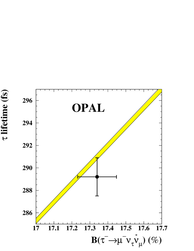
Figure 5: The lifetime of the $\tau$ vs the $\tau^{-}\rightarrow\mu^{-}\bar{\nu}_{\mu}\nu_{\tau}$ branching ratio. The band is the Standard Model expectation, and its width is determined by the uncertainty in the mass of the $\tau$ [19]. The point with error bars is the OPAL measurement of the $\tau$ lifetime [18] and the branching ratio determined in this work.

again in good agreement with the Standard Model assumption of lepton universality. If one assumes lepton universality, then Equation 3 can be rearranged to express the $\tau$ lifetime as a function of the branching ratio B($\tau^{-}\rightarrow\mu^{-}\bar{\nu}_{\mu}\nu_{\tau}$). The resulting relationship is plotted in Figure 5.

6.2 Michel parameter $\eta$ and the charged Higgs mass

The leptonic $\tau$ branching ratios can be used to probe the Lorentz structure of the matrix element through the Michel parameters [3, 20], $\eta$, $\rho$, $\xi$, and $\delta$, which parameterize the shape of the $\tau$ leptonic decay spectrum. In the Standard Model V-A framework, $\eta$ takes the value zero. A non-zero value of $\eta$ would contribute an extra term to the leptonic $\tau$ decay widths. This effect potentially would be measurable by taking the ratio of branching ratios, as in Equation 4 [21],

$$\frac{\mbox{B($\tau^{-}\rightarrow\mu^{-}\bar{\nu}_{\mu}\nu_{\tau}$)}}{\mbox{B}(\tau^{-}\rightarrow\mbox{e}^{-}\bar{\nu}_{e}\nu_{\tau})}=0.9726\left(1+4\eta\frac{m_{\mu}}{m_{\tau}}\right).$$ (4)

The B($\tau^{-}\rightarrow\mu^{-}\bar{\nu}_{\mu}\nu_{\tau}$)  result presented here, together with the OPAL measurement of B$(\tau^{-}\rightarrow\mbox{e}^{-}\bar{\nu}_{e}\nu_{\tau})$ [1] and Equation 4, then results in a value of $\eta=0.004\pm 0.037$. This can be compared with a previous OPAL result of $\eta=0.027\pm 0.055$ [3] which has been obtained by fitting the $\tau$ decay spectrum.

In addition, a non-zero $\eta$ may imply the presence of scalar couplings, such as those predicted in the Minimal Supersymmetric Standard Model. The dependence of $\eta$ upon the mass of the charged Higgs particle in this model, $m_{\mathrm{H}^{\pm}}$, can be approximately written as [21, 22]

$$\eta=-\frac{m_{\tau}m_{\mu}}{2}\left(\frac{\tan\beta}{m_{\mathrm{H}^{\pm}}}\right)^{2},$$ (5)

where $\tan\beta$ is the ratio of the vacuum expectation values of the two Higgs fields. Thus, $\eta$ can be used to place constraints on the mass of the charged Higgs. A one-sided 95% confidence limit using the $\eta$ evaluated in this work gives a value of $\eta>-0.057$, and a model-dependent limit on the charged Higgs mass of $m_{\mathrm{H}^{\pm}}>1.28\tan\beta$.

7 Conclusions

OPAL data collected at energies near the Z⁰ peak have been used to determine the $\tau^{-}\rightarrow\mu^{-}\bar{\nu}_{\mu}\nu_{\tau}$ branching ratio, which is found to be

$$\mbox{B($\tau^{-}\rightarrow\mu^{-}\bar{\nu}_{\mu}\nu_{\tau}$)}=0.1734\pm 0.0009(stat)\pm 0.0006(syst).$$

This is the most precise measurement to date, and is consistent with the previous OPAL measurement [2] and with previous results from other experiments [15].

The branching ratio measured in this analysis, in conjunction with the OPAL $\tau^{-}\rightarrow\mbox{e}^{-}\bar{\nu}_{e}\nu_{\tau}$ branching ratio measurement, has been used to verify lepton universality at the level of 0.5%. Although lepton universality has been tested to precisions of 0.2% using pion decays, the scalar nature of pions constrains the mediating W boson to be longitudinal, whereas $\tau$ decays involve transverse W bosons, making these two universality tests potentially sensitive to different types of new physics.

In addition, these branching ratios have been used to obtain a value for the Michel parameter $\eta=0.004\pm 0.037$, which in turn has been used to place a limit on the mass of the charged Higgs boson, $m_{\mathrm{H}^{\pm}}>1.28\tan\beta$, in the Minimal Supersymmetric Standard Model. This result is complementary to that from another recent OPAL analysis [23], where a limit of $m_{\mathrm{H}^{\pm}}>1.89\tan\beta$ has been obtained from the decay $b\rightarrow\tau^{-}\bar{\nu}_{\tau}\mathrm{X}$.

Figure 1: (a, b) The number of muon layers, $N_{\mathrm{muon}}$, activated by the passage of a charged particle in the jet, and (c, d) the $\mu_{\mathrm{match}}$ matching between a muon track reconstructed in the tracking chamber and one reconstructed in the muon chamber. The jets in each plot have passed all other selection criteria. The arrows indicate the accepted regions. The points are data, the clear histogram is the Monte Carlo $\tau^{-}\rightarrow\mu^{-}\bar{\nu}_{\mu}\nu_{\tau}$ prediction, the singly-hatched histogram is the Monte Carlo prediction for backgrounds from other $\tau$ decays, and the cross-hatched histogram is the Monte Carlo prediction for background from non-$\tau$ sources.

Figure 2: (a) The momentum of the highest momentum particle in the opposite jet, $p_{\mathrm{1-opp}}$, where the candidate muon has a momentum greater than 40 GeV/c, and (b) the combined momentum of the second and third particles in those jets which have more than one track, for jets which have passed all other selection criteria. The arrows indicate the accepted regions. The points are data, the clear histogram is the Monte Carlo $\tau^{-}\rightarrow\mu^{-}\bar{\nu}_{\mu}\nu_{\tau}$ prediction, the singly-hatched histogram is the Monte Carlo prediction for backgrounds from other $\tau$ decays, and the cross-hatched histogram is the Monte Carlo prediction for background from non-$\tau$ sources.

Figure 3: The momentum of the candidate muon, $p_{\mathrm{\mu}}$, for jets which have passed all of the selection criteria. The points are data, the clear histogram is the Monte Carlo $\tau^{-}\rightarrow\mu^{-}\bar{\nu}_{\mu}\nu_{\tau}$ prediction, the singly-hatched histogram is the Monte Carlo prediction for backgrounds from other $\tau$ decays, and the cross-hatched histogram is the Monte Carlo prediction for background from non-$\tau$ sources.

Figure 4: The distributions used to measure the background in the $\tau^{-}\rightarrow\mu^{-}\bar{\nu}_{\mu}\nu_{\tau}$ sample are shown after the normalization. The arrows indicate the region that was chosen to measure each background. (a) $E_{\mathrm{jet}}$ is the energy measured in the electromagnetic calorimeter, (b) $\theta_{\mathrm{acol}}$ is the acollinearity angle between the two $\tau$ jets, (c) $p_{\mathrm{1-opp}}$ is the momentum of the highest momentum particle in the opposite jet to the $\tau^{-}\rightarrow\mu^{-}\bar{\nu}_{\mu}\nu_{\tau}$ candidate, (d) $\mathrm{d}E/\mathrm{d}x$ is the rate of energy loss of a particle traversing the tracking chamber. The points are data, the clear histogram is the Monte Carlo $\tau^{-}\rightarrow\mu^{-}\bar{\nu}_{\mu}\nu_{\tau}$ prediction, the singly-hatched histogram is the Monte Carlo prediction for the type of background being evaluated using each distribution, and the cross-hatched histogram is the Monte Carlo prediction for all other types of background.

References

- [1] OPAL Collaboration, G. Abbiendi et al., Phys. Lett. B447 (1999) 134.
- [2] OPAL Collaboration, R. Akers et al., Z. Phys. C66 (1995) 543.
- [3] OPAL Collaboration, K. Ackerstaff et al., Eur. Phys. J. C8 (1999) 3.
- [4] OPAL Collaboration, G. Alexander et al., Phys. Lett. B388 (1996) 437.
-
[5]
OPAL Collaboration, K. Ahmet et al., Nucl. Inst. and
Meth. A305 (1991) 275;
OPAL Collaboration, P.P. Allport et al., Nucl. Inst. and Meth. A324 (1993) 34;
OPAL Collaboration, P.P. Allport et al., Nucl. Inst. and Meth. A346 (1994) 476. - [6] S. Jadach, B.F.L. Ward, and Z. Wa̧s, Comp. Phys. Comm. 79 (1994) 503.
- [7] S. Jadach et al., Comp. Phys. Comm. 76 (1993) 361.
- [8] J. Allison et al., Nucl. Inst. and Meth. A317 (1992) 47.
- [9] T. Sjöstrand, Comp. Phys. Comm. 82 (1994) 74.
- [10] S. Jadach, W. Placzek, and B.F.L. Ward, Phys. Lett. B390 (1997) 298.
-
[11]
R. Bhattacharya, J. Smith, and G. Grammer,
Phys. Rev. D15 (1977) 3267;
J.A.M. Vermaseren, and G. Grammer, Phys. Rev. D15 (1977) 3280. -
[12]
OPAL Collaboration, G. Alexander et al.,
Phys. Lett. B266 (1991) 201;
OPAL Collaboration, P. Acton et al., Phys. Lett. B288 (1992) 373. - [13] OPAL Collaboration, G. Abbiendi et al., Eur. Phys. J. C19 (2001) 587.
- [14] OPAL Collaboration, G. Alexander et al., Z. Phys. C52 (1991) 175.
- [15] Particle Data Group, D.E. Groom et al., Eur. Phys. J. C15 (2000) 1.
- [16] OPAL Collaboration, K. Ackerstaff et al., Eur. Phys. J. C4 (1998) 193.
- [17] W.J. Marciano and A. Sirlin, Phys. Rev. Lett. 61 (1988) 1815.
- [18] OPAL Collaboration, G. Alexander et al., Phys. Lett. B374 (1996) 341.
- [19] BES Collaboration, J.Z. Bai et al., Phys. Rev. D53 (1996) 20.
- [20] L. Michel, Proc. Phys. Soc. A63 (1950) 514.
- [21] A. Stahl, Phys. Lett. B324 (1994) 121 and references therein.
- [22] M.T. Dova, J. Swain and L. Taylor, Nucl. Phys. B (Proc. Suppl.) 76 (1999) 133.
- [23] OPAL Collaboration, G. Abbiendi et al., Phys. Lett. B520 (2001) 1.