Measurement of the $B^{0}-\overline{B}^{0}$ mixing rate with $B^{0}(\overline{B}^{0})\to D^{*\mp}\pi^{\pm}$ partial reconstruction

Abstract

We report a measurement of the $B^{0}-\overline{B}^{0}$ mixing parameter $\Delta m_{d}$ based on a $\rm 29.1~{}fb^{-1}$ sample of $\Upsilon(4S)$ resonance decays collected by the Belle detector at the KEKB asymmetric $e^{+}e^{-}$ collider. We use events with a partially reconstructed $B^{0}(\overline{B}^{0})\to D^{*\mp}\pi^{\pm}$ candidate and where the flavor of the accompanying $B$ meson is identified by the charge of the lepton from a $B^{0}(\overline{B}^{0})\to X^{\mp}\ell^{\pm}\nu$ decay. The proper-time difference between the two $B$ mesons is determined from the distance between the two decay vertices. From a simultaneous fit to the proper-time distributions for the same-flavor ($B^{0}(\overline{B}^{0})$, $\ell^{\pm}$) and opposite-flavor ($B^{0}(\overline{B}^{0})$, $\ell^{\mp}$) event samples, we measure the mass difference between the two mass eigenstates of the neutral $B$ meson to be $\Delta m_{d}$= $(0.509\pm 0.017~{}(\rm stat)\pm 0.020~{}(\rm syst))~{}ps^{-1}$.

I INTRODUCTION

After production, $B^{0}$ and $\overline{B}^{0}$ mesons evolve in time and mix into each other via the second-order weak interaction box diagrams shown in Fig. 1.

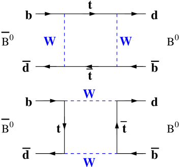
Figure 1: Standard Model “box diagrams” for the second-order weak $B^{0}-\overline{B}^{0}$ mixing process.

The mixing parameter $\Delta m_{d}$, which is the mass difference of the two neutral $B$ mass eigenstates, is determined from the Feynman diagrams shown in Fig. 1 Sandabook to be

$$\Delta m_{d}=\frac{G^{2}_{F}}{6\pi^{2}}f^{2}_{B}m_{B}m^{2}_{W}\eta_{t}S|V^{*}_{tb}V_{td}|^{2}B_{B}~{},$$ (1)

where $m_{t}$, $m_{B}$ and $m_{W}$ are the $t$-quark, $B^{0}$ and $W$ masses; $G_{F}$ is the Fermi constant; $\eta_{t}$ is a QCD correction buras1 ; $S$ is a function of ${m_{t}^{2}}/{m_{W}^{2}}$ Inamiburas2 ; $f_{B}$ is the decay constant of the $B$ meson; and $B_{B}$ is the $B$ meson bag parameter donoghue . In principle, a measurement of the mixing parameter $\Delta m_{d}$ can be used to determine the magnitude of the CKM matrix element $|V_{td}|$. However, there are large theoretical uncertainties associated with the model dependence of $f_{B}$ and $B_{B}$. We report here a measurement of $\Delta m_{d}$ that uses $B$ mesons from the decays of $\Upsilon(4S)$ states produced by the KEKB collider and recorded in the Belle detector. We determine the flavor of one $B$ meson by partially reconstructing the decays $B^{0}(\overline{B}^{0})\to D^{*\mp}\pi^{\pm}$; the flavor of the accompanying $B$ meson is identified by the charge of the lepton from $B^{0}(\overline{B}^{0})\to X^{\mp}\ell^{\pm}\nu$ decays. In the future, this technique can be extended to determine the linear combination of CKM angles $2\phi_{1}+\phi_{3}$ dunietz .

The $\Upsilon(4S)$ decays to a $B^{0}-\overline{B}^{0}$ pair that is nearly at rest in the $\Upsilon(4S)$ center of mass system (CM). Since $B$ mesons are spin 0 mesons, angular momentum conservation requires the two $B$ mesons to be in an antisymmetric quantum state

$$|\alpha\rangle=\frac{1}{\sqrt{2}}\left(|B^{0}(1)\rangle|\overline{B}^{0}(2)\rangle-|\overline{B}^{0}(1)\rangle|B^{0}(2)\rangle\right),$$ (2)

where 1 and 2 indicate the opposite sides in the $\Upsilon(4S)$ decay plane. The form of Eq. (2) guarantees that at any time the amplitude for either $B^{0}B^{0}$ or $\overline{B}^{0}\overline{B}^{0}$ states vanishes. Thus, if we determine the flavor and decay time $t_{tag}$ for one of the $B$ mesons to decay into a final state $f_{tag}$, then we can measure the time evolution of the other $B$ at any time $t$ as a function of the time difference $\Delta t=t-t_{tag}$. For the two-state neutral $B$ system, the following probability expressions hold to a good approximation Sandabook ,

$$\hskip 19.91692pt\matrix{{\rm P}^{\rm OF}(\Delta t)&=&{1\over{4\tau_{B^{0}}}}{e^{-{|\Delta t|\over\tau_{B^{0}}}}\left[1+\cos(\Delta m_{d}\Delta t)\right]~{},}\\ {\rm P}^{\rm SF}(\Delta t)&=&{1\over{4\tau_{B^{0}}}}{e^{-{|\Delta t|\over\tau_{B^{0}}}}\left[1-\cos(\Delta m_{d}\Delta t)\right]~{},}}\hskip-19.91692pt$$

where the superscripts SF and OF denote events where the lepton-tagged and partially reconstructed $B$ mesons have the same and opposite flavors, respectively.

Since the $B^{0}$ and $\overline{B}^{0}$ are nearly at rest in the CM frame, $\Delta t$ can be determined from the displacement between the lepton-tagged and partially reconstructed $B$ decay vertices

$$\Delta t\simeq(z_{\rm rec}-z_{\rm tag})/\beta\gamma c\equiv\Delta z/\beta\gamma c,$$ (3)

where the $z$ axis is defined to be anti-parallel to the positron beam direction and the constant $\beta\gamma=0.425$ is the Lorentz boost of the $e^{+}e^{-}$ center of mass system at the KEKB collider.

This paper is organized as follows: In Section II, we describe the KEKB collider and the Belle detector. The partial reconstruction of $B^{0}(\overline{B}^{0})\to D^{*\mp}\pi^{\pm}$ decays, the determination of the $b$-flavor of the accompanying $B$ meson and the measurement of $\Delta t$ are described in Section III. The likelihood fit to the measured $\Delta t$ distributions is described in Section IV. We present the results of the fit and studies of sources of systematic errors in Sections V, VI and VII. The conclusions are presented in Section VIII.

II EXPERIMENTAL APPARATUS

KEKB KEKB is an asymmetric $e^{+}e^{-}$ collider 3 km in circumference, which consists of 8 GeV $e^{-}$ and 3.5 GeV $e^{+}$ storage rings and an injection linear accelerator. It has a single interaction point (IP) where the $e^{+}$ and $e^{-}$ beams collide with a crossing angle of 22 mrad. The collider has reached a peak luminosity above 8$\times 10^{33}$ cm^-2s^-1. Due to the energy asymmetry, the $\Upsilon(4S)$ resonance and its daughter $B$ mesons are produced with a Lorentz boost of $\beta\gamma=$0.425. On average, the $B$ mesons decay approximately 200 $\mu$m from the $\Upsilon(4S)$ production point.

The Belle detector Belle is a general-purpose large solid angle magnetic spectrometer surrounding the interaction point. Precision tracking and vertex measurements are provided by a silicon vertex detector (SVD) SVD and a central drift chamber (CDC) CDC in a 1.5 T magnetic field parallel to the $z$-axis. The SVD consists of three layers of double-sided silicon strip detectors (DSSD) arranged in a barrel and covers 86% of the solid angle. The three layers at radii of 3.0, 4.5 and 6.0 cm surround the beam-pipe, a double-wall beryllium cylinder of 2.3 cm radius and 1 mm thickness. The strip pitches of each DSSD are 84 $\mu$m for the measurement of the $z$ coordinate and 25 $\mu$m for the measurement of the $r-\phi$ coordinate. The CDC is a small-cell cylindrical drift chamber with 50 layers of anode wires including 18 layers of stereo wires. A low-$Z$ gas mixture ($\mathrm{He}$(50%)$+\mathrm{C}_{2}\mathrm{H}_{6}$(50%)) is used to minimize multiple Coulomb scattering to ensure good momentum resolution, especially for low momentum particles. The CDC provides three-dimensional trajectories of charged particles in the polar angle region $17^{\circ}<\theta<150^{\circ}$ in the laboratory frame. The impact parameter resolution for reconstructed tracks is measured as a function of the track momentum $p$ (measured in GeV/c) to be $\sigma_{xy}$ = [19 $\oplus$ 50/($p\beta\sin^{3/2}\theta$)] $\mu$m and $\sigma_{z}$ = [36 $\oplus$ 42/($p\beta\sin^{5/2}\theta$)] $\mu$m. The momentum resolution of the combined tracking system is $\sigma_{p_{t}}/p_{t}=(0.30/\beta\oplus 0.19p_{t})$%, where $p_{t}$ is the transverse momentum in GeV/c.

The identification of charged pions and kaons uses three detector systems: the CDC measuring $dE/dx$, a set of time-of-flight counters (TOF) TOF and a set of aerogel Cherenkov counters (ACC) ACC . The CDC measures energy loss for charged particles with a resolution of $\sigma(dE/dx)$ = 6.9% for minimum-ionizing pions. The TOF consists of 128 plastic scintillators viewed on both ends by fine-mesh photo-multipliers that operate stably in the 1.5 T magnetic field. Their time resolution is 95 ps ($rms$), providing three standard deviation (3$\sigma$) $K^{\pm}/\pi^{\pm}$ separation below 1.0 GeV/$c$, and 2$\sigma$ separation up to 1.5 GeV/$c$. The ACC consists of 1188 aerogel blocks with refractive indices between 1.01 and 1.03 depending on the polar angle. Fine-mesh photo-multipliers detect the Cherenkov light. The effective number of photoelectrons is approximately 6 for $\beta=1$ particles. Using the information from these three particle identification systems, the $K/\pi$ likelihood ratio $P(K/\pi)={\cal{L}}(K)/({\cal{L}}(K)+{\cal{L}}(\pi))$ is calculated, where ${\cal{L}}(K)$ and ${\cal{L}}(\pi)$ are kaon and pion likelihoods Belle . A selection with $P(K/\pi)>0.6$ retains about 90% of the charged kaons with a charged pion misidentification rate of about 6%.

Photons and other neutral particles are reconstructed in a CsI(Tl) crystal calorimeter (ECL) ECL consisting of 8736 crystal blocks, 16.2 radiation lengths ($X_{0}$) thick. Electron identification is based on a combination of $dE/dx$ measurements in the CDC, the response of the ACC, the position and the shape of the electromagnetic shower, as well as the ratio of the cluster energy to the particle momentum EID . For the electron identification requirement used in this analysis, the electron identification efficiency is determined from two-photon $e^{+}e^{-}\rightarrow e^{+}e^{-}e^{+}e^{-}$ processes to be more than 90% for $p_{\rm lab}>1.0$ GeV/c. The hadron misidentification probability, determined using tagged pions from inclusive $K_{S}^{0}\rightarrow\pi^{+}\pi^{-}$ decays, is below $0.5\%$.

All the detectors mentioned above are inside a super-conducting solenoid of 1.7 m radius. The outermost spectrometer subsystem is a $K_{L}^{0}$ and muon detector (KLM) KLM , that consists of 14 layers of iron (4.7 cm thick) absorber alternating with resistive plate counters (RPC). The KLM system covers polar angles between 20 and 155 degrees. The efficiency of the muon identification requirement used here, determined by using the two-photon process $e^{+}e^{-}\rightarrow e^{+}e^{-}\mu^{+}\mu^{-}$ and simulated muons embedded in $B\overline{B}$ candidate events, is greater than 90% for tracks with $p_{\rm lab}>1$ GeV/c. The corresponding pion misidentification probability, determined using $K_{S}^{0}\rightarrow\pi^{+}\pi^{-}$ decays, is less than 2%.

In our analysis, Monte Carlo (MC) events are generated using the $QQ$ event generator QQ and the response of the Belle detector is precisely simulated by a GEANT3-based program GEANT . The simulated events are then reconstructed and analyzed with the same procedure as is used for the real data.

III EVENT RECONSTRUCTION

III.1 Data Sample

We analyze a $29.1~{}\rm fb^{-1}$ data sample recorded on the $\Upsilon(4S)$ resonance. The data was taken from June 1999 to July 2001 and corresponds to about $3.13\times 10^{7}$ $B\overline{B}$ pairs.

III.2 $B\overline{B}$ Event Pre-selection

In Belle, neutral $B$ mesons can only be created via the process $\Upsilon(4S)\to B^{0}\overline{B}^{0}$. To suppress the non-$b\overline{b}$ background processes from QED, beam-gas and $e^{+}e^{-}\to\tau^{+}\tau^{-}$, we select hadronic events using event multiplicity and total energy variables hadsel .

III.3 $B\to D^{*}\pi$ Decay Partial Reconstruction

We now describe a partial reconstruction method for the decay chain $B\to D^{*}\pi_{f}$, $D^{*}\to D\pi_{s}$, where $\pi_{f}$ and $\pi_{s}$ designate a fast $\pi$ and slow $\pi$, respectively. This is a variation of a technique that was first developed by the CLEO collaboration partial . For the Belle experiment, we modify and apply this method to make a precise time dependent measurement of $\Delta m_{d}$. Unlike analyses that use fully reconstructed $B\to D^{*}\pi_{f}$ decays, we do not use any properties of the decay products of the $D^{0}$ meson in the decay $D^{*}\to D\pi_{s}$. According to a Monte Carlo simulation, this method yields an order of a magnitude more events than a full reconstruction method.

III.3.1 Kinematics

We consider five particles in the decay chain: $B,D^{*},\pi_{f},D$ and $\pi_{s}$. When reconstructed in this way, the system has $20$ degrees of freedom.

For partial reconstruction, only the $\pi_{f}$ and $\pi_{s}$ are used. The $D$ candidate is not reconstructed. We can obtain constraints from 4-momentum conservation for both the decays $B\to D^{*}\pi_{f}$ and $D^{*}\to D\pi_{s}$ (8 constraints). The $B,~{}D^{*},~{}D,~{}\pi_{f}$ and $\pi_{s}$ masses from the PDG2000 compilation PDG2000 provide further 5 constraints. In addition, we use the constraint that the $B$ energy is the CM beam energy of KEKB at the $\Upsilon(4S)$ divided by 2 (1 constraint). The measurements of the $\pi_{f}$ and $\pi_{s}$ 3-vectors provide 6 constraints. In total there are 20 constraints, equal to the number of degrees of freedom of the system. Following previous analyses partial ; zyh , we use two variables to measure the $B\to D^{*}\pi$ signal. The first is $D^{0}$ missing mass,

$$M_{D_{miss}}^{2} = m_{B}^{2}+m_{\pi_{f}}^{2}+m_{\pi_{s}}^{2}-2E_{B}E_{\pi_{f}}-2E_{B}E_{\pi_{s}}$$

$$+ 2E_{\pi_{f}}E_{\pi_{s}}+2|\vec{p}_{B}||\vec{p}_{\pi_{f}}|\cos\theta_{B\pi_{f}}$$

$$+ 2|\vec{p}_{B}||\vec{p}_{\pi_{s}}|\cos\theta_{B\pi_{s}}-2|\vec{p}_{\pi_{f}}||\vec{p}_{\pi_{s}}|\cos\theta_{\pi_{f}\pi_{s}},$$

where $E,~{}\vec{p},~{}m$ are the energy, momentum and nominal masses for the $B,~{}D^{*},~{}D,~{}\pi_{f}$ and $\pi_{s}$ mesons in the CM frame; $\theta_{B\pi_{f(s)}}$ is the angle between the directions of motion of the $B$ and $\pi_{f(s)}$; and $\theta_{\pi_{f}\pi_{s}}$ is the angle between the $\pi_{f}$ and $\pi_{s}$. In the CM frame, $\cos\theta_{B\pi_{s}}\approx-\cos\theta_{B\pi_{f}}$; the analysis zyh shows that this approximation, and the relation

$$\cos\theta_{B\pi_{f}}={{-m_{B}^{2}-m_{\pi_{f}}^{2}+m_{D^{*}}^{2}+2E_{B}E_{\pi_{f}}}\over{2|\vec{p}_{B}||\vec{p}_{\pi_{f}}|}},$$ (5)

can be used to evaluate $M_{D_{miss}}$ without reconstructing the $B$ meson’s flight direction. The second variable is the angle $\theta_{\pi_{s}}^{*}$ between the slow pion in the $D^{*}$ rest frame and the direction of motion of the $D^{*}$ in the CM frame. Using partial reconstruction, it is calculated using the relation,

$$\cos\theta_{\pi_{s}}^{*}={{\beta_{D^{*}}(E_{D}^{*}-E_{\pi_{s}}^{*})}\over{2|\vec{p}_{\pi_{s}}^{\>*}|}}-{{|\vec{p}_{D}|^{2}-|\vec{p}_{\pi_{s}}|^{2}}\over{2\gamma_{D^{*}}^{2}\beta_{D^{*}}m_{D^{*}}|\vec{p}_{\pi_{s}}^{\>*}|}},$$ (6)

where $\gamma_{D^{*}}\equiv{E_{D^{*}}/m_{D^{*}}}=\left(E_{B}-\sqrt{|\vec{p}_{\pi_{f}}|^{2}+m_{\pi_{f}}^{2}}\right)/m_{D^{*}}$, $\beta_{D^{*}}\equiv\sqrt{1-\left(1/\gamma_{D^{*}}^{2}\right)}$ and $|\vec{p}_{D}|=\sqrt{E_{D}^{2}-m_{D}^{2}}=\sqrt{(E_{B}-E_{\pi_{f}}-E_{\pi_{s}})^{2}-m_{D}^{2}}$; $E_{D}^{*}$ and $E_{\pi_{s}}^{*}$ are the energy of $D$ and $\pi_{s}$ in the $D^{*}$ rest frame; $\vec{p}_{\pi_{s}}^{\>*}$ is the momentum of $\pi_{s}$ in the $D^{*}$ rest frame. The asterisks denote variables calculated in the $D^{*}$ rest frame. Calculated in this way, $\cos\theta_{\pi_{s}}^{*}$ can take values outside the physical region due to finite resolutions, or for background events.

III.3.2 $B^{0}(\overline{B}^{0})\to D^{*\mp}\pi^{\pm}$ Event Selection

The $B^{0}(\overline{B}^{0})\to D^{*\mp}\pi^{\pm}$ candidates are reconstructed with the following requirements. In the CM frame, we select $\pi_{f}$ candidates with momentum $\vec{p}_{\pi_{f}}$ in the range $2.05{\rm~{}GeV}/c<|\vec{p}_{\pi_{f}}|<2.45{\rm~{}GeV}/c$ and an oppositely charged $\pi_{s}$ with momentum $|\vec{p}_{\pi_{s}}|$ less than $0.45{\rm~{}GeV}/c$. We require $dr<0.05~{}\rm cm$, $dz<2\rm~{}cm$ for the $\pi_{f}$ candidate and $dr<0.2~{}\rm cm$, $dz<2\rm~{}cm$ for the $\pi_{s}$ candidate to suppress backgrounds from beam particles that interact with the residual gas of the vacuum system or spent-beam particles that strike the vacuum chamber wall. The variables $dr$ and $dz$ are the distances of closest approach of the track to the interaction point in the $r-\phi$ and $z$ planes, respectively. For better vertex resolution, the SVD is required to provide at least 2 spatial points for a $\pi_{f}$ candidate track. The $\pi_{f}$ candidates are required to have electron and muon likelihood ratios less than 0.8 to suppress background from semileptonic $B$ decays. Angular momentum conservation in the pseudoscalar to vector-pseudoscalar decay $B^{0}\to D^{*-}\pi^{+}$ leads to a distribution proportional to $\cos^{2}\theta^{*}_{\pi_{s}}$ for the angle $\theta^{*}_{\pi_{s}}$. To enhance the signal to background ratio, we require $0.3<|\cos\theta^{*}_{\pi_{s}}|<1.05$. We then select $B^{0}\to D^{*-}\pi^{+}$ candidates with $D^{0}$ missing mass $M_{D_{miss}}$ greater than $1.85~{}{\rm GeV}/c^{2}$ and $0.3<|\cos\theta^{*}_{\pi_{s}}|<1.05$. These two requirements define the signal region.

$\rm\cos\theta_{-\pi_{f}\pi_{s}}-\cos\theta_{-\pi_{f}D^{*}}\cos\theta_{\pi_{s}D^{*}}$

Figure 2: $\cos\theta_{-\pi_{f}\pi_{s}}-\cos\theta_{-\pi_{f}D^{*}}\cos\theta_{\pi_{s}D^{*}}$ distributions in a simulation of fully reconstructed Monte Carlo events.

Fig. 2 shows that the signal peaks at zero in the variable $|\cos\theta_{-\pi_{f}\pi_{s}}-\cos\theta_{-\pi_{f}D^{*}}\cos\theta_{\pi_{s}D^{*}}|$ zyh . For about $4\%$ of the events, more than one pair of opposite sign particles satisfy all the selection requirements. In these cases, we select the combination with the smallest value of $|\cos\theta_{-\pi_{f}\pi_{s}}-\cos\theta_{-\pi_{f}D^{*}}\cos\theta_{\pi_{s}D^{*}}|$. $\theta_{-\pi_{f}\pi_{s}},~{}\theta_{-\pi_{f}D^{*}}$ and $\theta_{\pi_{s}D^{*}}$ are the angles between the directions of $-\vec{p}_{\pi_{f}}$, $\vec{p}_{D^{*}}$ and $\vec{p}_{\pi_{s}}$ in the $B\to D^{*}\pi_{f}$, $D^{*}\to D\pi_{s}$ decay, respectively. This quantity is zero when the direction of the $\pi_{s}$ is a good approximation to the $D^{*}$ direction and is small when the plane defined by the $\vec{p}_{D^{*}}$ and $\vec{p}_{\pi_{s}}$ nearly coincides with the plane defined by the $\vec{p}_{D^{*}}$ and $-\vec{p}_{\pi_{f}}$.

III.4 Flavor Tagging for neutral $B$ meson

The flavor of the signal $B$ decay is obtained from the charge of the fast pion. The flavor of the accompanying $B$ meson decay is determined from the charge of the primary lepton ($e$ or $\mu$) from the semileptonic decay $b\to c\ell^{-}\nu$. In addition to tagging the flavor of the $B$ meson decay, there are two other major reasons for using a high-momentum lepton: the point of closest approach of the lepton track and the beam-line provides the location of the tagging side vertex; the requirement of a high momentum lepton in the event dramatically reduces the continuum background.

We require the lepton to have a momentum in the CM frame of at least ${\rm 1.1~{}GeV/}c$. We select leptons from well measured tracks by requiring $dr<0.05\rm~{}cm$, $dz<2\rm~{}cm$. We demand that the lepton have both $r-\phi$ and $z$ hits in the SVD. To reject secondary leptons from the decay of the unreconstructed $D^{0}$ mesons, we require the cosine of the angle between the lepton and $\pi_{f}$ to be greater than $-0.8$. We also reject lepton tracks that, when combined with any other oppositely charged track in the event, have an invariant mass that is within $\rm 50~{}MeV$ of the $J/\psi$ mass. If more than one lepton in an event satisfies all of the above criteria, the highest momentum lepton is selected.

However, not all lepton candidates are primary leptons. According to a MC study, the background is dominated by three sources. The first is secondary leptons from charm decays (“cascade leptons”) which come from the $b\to c\to s\ell^{+}\nu$ decay chain and not directly from $b\to c\ell^{-}\overline{\nu}$ like the “primary leptons”. The charges of the cascade and primary leptons are opposite and, thus, cascade leptons can bias the tagged flavor of $B$ mesons and must be well understood. Two of the requirements described above discriminate against secondary leptons: the momentum requirement and the angular cut with respect to the fast $\pi$ direction. The second category of incorrect tags is due to leptons from $J/\psi$ and $\psi(2S)$ decays. Equal numbers of positively and negatively charged leptons are produced from $J/\psi$ and $\psi(2S)$ decays. Hence, the charge of the observed lepton is uncorrelated with the $B$ flavor. The third category is composed of hadronic tracks misidentified as leptons. Particle identification is applied to suppress this background.

III.5 Vertex Reconstruction

An analysis that relies on $\Delta t$ information requires a measurement of $\Delta t$ in Eq. (I). We use the $z$ difference between $B$ decay vertices in the laboratory system to approximate the proper-time difference $\Delta t$ by

$$\Delta z\equiv z_{\pi_{f}}-z_{l}=\gamma(\Delta z_{CM}+c\beta\Delta t)\simeq c\beta\gamma\Delta t~{},$$ (7)

where $z_{\pi_{f}}$ and $z_{l}$ are the $z$ positions of the fast pion and lepton tracks respectively, and $c$ is the speed of light. The constant $\beta\gamma=0.425$ is the Lorentz boost factor for the $e^{+}e^{-}$ center of mass system in the Belle experiment. $\Delta z_{CM}$ is the $z$ difference between $B$ decay vertices in the CM frame. Here, we assume that the $B$ mesons are at rest in the CM frame and thus $\Delta z_{CM}\simeq 0$. Therefore we have

$$\Delta t\simeq\frac{\Delta z}{c\beta\gamma}~{}.$$ (8)

The $z$ positions are determined from the intersection of the $\rm\pi_{f}$ (or lepton track) with the profile of $B$ decay vertices, which is estimated run-by-run from the profile of the interaction point ($\sigma^{IP}_{x}\sim 110~{}\mu{\rm m},~{}\sigma^{IP}_{y}\sim 5~{}\mu{\rm m},~{}\sigma^{IP}_{z}\sim 3500~{}\mu{\rm m}$) convolved with the average $B$ flight length ($30~{}\mu$m in the CM frame).

III.6 Signal

Monte Carlo simulation shows that $B^{0}(\overline{B}^{0})\to D^{*\mp}\rho^{\pm}$ candidates are peaked around $1.865~{}{\rm GeV}/c^{2}$ in the $D^{0}$ missing mass distribution, the same location as $B^{0}(\overline{B}^{0})\to D^{*\mp}\pi^{\pm}$ decays. $B^{0}(\overline{B}^{0})\to D^{*\mp}\rho^{\pm}$ decays can also be treated as signal for the measurement of $B^{0}-\overline{B}^{0}$ mixing. Thus, the signal consists of $B^{0}(\overline{B}^{0})\to D^{*\mp}\pi^{\pm}$ and $B^{0}(\overline{B}^{0})\to D^{*\mp}\rho^{\pm}$ decays tagged by primary leptons. Henceforth, for simplicity we use the notation $B^{0}(\overline{B}^{0})\to D^{*\mp}h^{\pm}$ to represent both $B^{0}(\overline{B}^{0})\to D^{*\mp}\pi^{\pm}$ and $B^{0}(\overline{B}^{0})\to D^{*\mp}\rho^{\pm}$ decays.

III.7 Backgrounds

Some other decay modes, such as $B^{0}\to D^{**-}\pi^{+}$ and $B^{0}\to D^{*-}l^{+}\nu_{l}$, also peak in $D^{0}$ missing mass, and hence can fake the signal. We therefore divide the backgrounds into unpeaked and peaked categories. Unpeaked background is dominated by random combinations of $\pi_{f}$ and $\pi_{s}$ with primary leptons from $B^{0}$ and $B^{\pm}$ decays, and combinatorial background from continuum. We verify in MC that the $\Delta z$ shape of the unpeaked background can be modeled by the $D^{0}$ missing mass sideband. The $\Delta z$ shapes of unpeaked background thus are taken from the $D^{0}$ missing mass sideband. The peaked background is dominated by the following sources: signal $B$ decays ($B^{0}(\overline{B}^{0})\to D^{*\mp}\pi^{\pm}$ and $B^{0}(\overline{B}^{0})\to D^{*\mp}\rho^{\pm}$) with secondary-lepton tags or fake-lepton tags; $B^{0}$ $\to$ $D^{**-}$ $\pi^{+}$, $B^{+}$ $\to$ $\overline{D}^{**0}$ $\pi^{+}$ and $B^{0}$ $\to$ $D^{*-}\pi^{+}\pi^{0}$ decays with primary-lepton tags, secondary-lepton tags or fake-lepton tags. The $\Delta z$ shapes of peaked background are determined from Monte Carlo simulation. The details of the background parameterization are described in Section IV.

III.8 Signal Yields

To obtain the signal yields, we apply a binned maximum likelihood fit to the $D^{0}$ meson missing mass distribution. In the fit, the signal shape is determined from the $B\to D^{*}\pi_{f}$ Monte Carlo simulation. The shape of the unpeaked background is taken from wrong-sign combinations, where the sign of the charges of the $\pi_{f}$ and $\pi_{s}$ are the same. The MC simulation shows that the wrong sign combinations have a distribution consistent with the right sign unpeaked background. The peaked background shape comes from the $B\overline{B}$ Monte Carlo simulation. In the fit, the shape of the signal, the peaked background and the unpeaked background are fixed. We also fix the peaked background normalization from the Monte Carlo simulation. We float the normalizations of the signal and unpeaked background. By fitting the $D^{0}$ missing mass distributions shown in Figs 3 and 4, we obtain signal yields of $3433\pm 81$ (SF: $751\pm 41$, OF: $2682\pm 70$). The estimated backgrounds (unpeaked/peaked) in the signal region are $1466\pm 37$ (SF: $243\pm 16$/$219\pm 15$, OF: $491\pm 18$/$513\pm 23$) for $M_{D_{miss}}>1.85$ GeV/$c^{2}$.

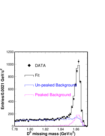
Figure 3: $D^{0}$ missing mass (GeV) distribution for lepton tagged $B^{0}\to D^{*-}h^{+}$ candidates.

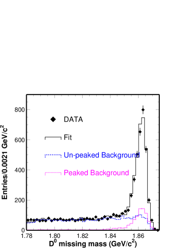
(a)

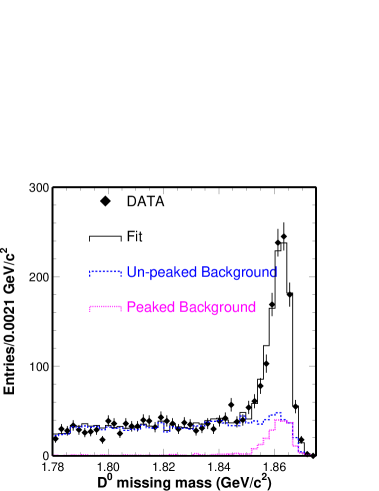
(b)

Figure 4: $D^{0}$ missing mass (${\rm GeV}/c^{2}$) distribution (a) for opposite flavor final states and (b) for the same flavor final states.

As a consistency check, we use another method to estimate the signal yields. In Fig. 5, we fit the $\cos\theta^{*}_{\pi_{s}}$ distribution with both signal and background shapes determined from MC. Here, we float both the signal and background normalizations. For the signal shape, we treat $B^{0}\to D^{*-}\pi^{+}$ and $B^{0}\to D^{*-}\rho^{+}$ events separately. The polarization of $B^{0}\to D^{*-}\rho^{+}$ is fixed from the CLEO measurement drho . We obtain $B^{0}\to D^{*-}\pi^{+}$ and $B^{0}\to D^{*-}\rho^{+}$ yields of $2454\pm 90$ and $1353\pm 96$ events. Note that the yields include incorrectly tagged signal. According to a MC study, the probability of incorrect tagging is $9.5\%$. Thus, we conclude that the two methods yield consistent results. Since the error is smaller for the yields obtained by fitting the $D^{0}$ missing mass distribution, we use the results from that method in the analysis.

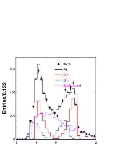
$\rm\cos\theta^{*}_{\pi_{s}}$

Figure 5: $\cos\theta^{*}_{\pi_{s}}$ distribution. The histogram from the fit and the contributions of signal and background are overlaid.

IV MAXIMUM LIKELIHOOD FIT

We extract the mixing frequency $\Delta m_{d}$ by simultaneously fitting the time evolution distribution of the SF and OF $B^{0}\to D^{*-}h^{+}$ samples. The unbinned maximum likelihood fitting method is applied to expressions containing $\Delta m_{d}$ as a free parameter, which take into account both signal and background.

IV.1 PDF and Likelihood Function

Here, we summarize the forms of signal and backgrounds used in the fitting. The likelihood is also established.

For the signal, the probability density functions (PDF) of OF and SF events are given by

$$F^{\rm OF}_{\rm sig}(\Delta t) = \int^{\infty}_{-\infty}{\rm P}^{\rm OF}(\Delta t^{\prime})R_{\rm sig}(\Delta t-\Delta t^{\prime})d\Delta t^{\prime}~{},$$ (9)

$$F^{\rm SF}_{\rm sig}(\Delta t) = \int^{\infty}_{-\infty}{\rm P}^{\rm SF}(\Delta t^{\prime})R_{\rm sig}(\Delta t-\Delta t^{\prime})d\Delta t^{\prime}~{},$$ (10)

where $R_{\rm sig}(\Delta t)$ is the signal resolution function, which is parameterized by a triple-Gaussian distribution as follows.

$$R_{\rm sig}(\Delta t) = f_{1}G(\Delta t;\mu_{1},\sigma_{1})+f_{2}G(\Delta t;\mu_{2},\sigma_{2})$$ (11)

$$+(1-f_{1}-f_{2})G(\Delta t;\mu_{3},\sigma_{3})~{}.$$

Here, $G(t;\mu,\sigma)$ is the Gaussian distribution, $f_{1}$ and $f_{2}$ denote the fractions of the first and second Gaussian, respectively. For the background, the PDFs include separate contributions for the parts that are peaked and unpeaked in the $D^{0}$ missing mass distribution. The time dependent parameterization includes prompt (zero lifetime) and finite lifetime components as well as $B^{0}-\overline{B}^{0}$ mixing. The time distribution of the unpeaked background is determined from the $D^{0}$ missing mass sideband data. The functional forms for the background PDFs are given in the appendix.

Using the PDFs described in Eqs. (9) (10) (15) and (16), the likelihood function can be written as

$${\cal L}=\prod_{i}\left((1-f_{\rm bkg})F^{\rm OF}_{\rm sig}(\Delta t_{i})+f_{\rm bkg}f^{\rm OF}_{\rm bkg}F_{\rm bkg}^{\rm OF}(\Delta t_{i})\right)\times$$ (12)

$$\prod_{j}\left((1-f_{\rm bkg})F^{\rm SF}_{\rm sig}(\Delta t_{j})+f_{\rm bkg}(1-f_{\rm bkg}^{\rm OF})F^{\rm SF}_{\rm bkg}(\Delta t_{j})\right)~{},$$

where $f_{\rm bkg}\equiv N_{\rm bkg}/(N_{\rm bkg}+N_{\rm sig})$ is the background fraction. $f_{\rm bkg}^{\rm OF}$ is the fraction of OF events in the background and calculated from $N_{\rm bkg}^{\rm OF}/N_{\rm bkg}$. The normalizations are determined from the fit to the $D^{0}$ missing mass distribution.

IV.2 Resolution Function

We need to determine the detector resolution function to smear the theoretical probability expressions in Eq. I. The signal resolution function $R_{\rm sig}(\Delta t)$ is the distribution of the difference between the generated and reconstructed $B^{0}$ decay proper times. A good approximation to the resolution function can be obtained from the reconstructed $\Delta z\equiv z_{l^{+}}-z_{l^{-}}$ distribution of $J/\psi\to l^{+}l^{-}$ decays in data, which were parameterized using the triple-Gaussian distribution in Eq. (11). In Monte Carlo simulation, Fig. 6 shows good agreement between the signal resolution function from “$D^{*-}\pi^{+}+l^{-}_{tag}$” events and the background subtracted $\Delta z$ distribution from $J/\psi\to l^{+}l^{-}$ decays. This indicates that using inclusive $J/\psi$ decays to model the tagged $D^{*}\pi$ resolution function is justified.

Figure 6: Resolution functions for $J/\psi\to l^{+}l^{-}$ decays and “$D^{*-}\pi^{+}+l^{-}_{tag}$” in MC.

$J/\psi\to l^{+}l^{-}$ candidates were selected using similar requirements to those in the “$B^{0}\to D^{*-}\pi^{+}+l^{-}_{tag}$” selection. The particle identification criteria are changed to select lepton pairs. Furthermore, no requirement is made on the angle between the tracks, since $J/\psi$ decays produce lepton pairs with large opening angles. In Fig. 7, the $J/\psi\to\mu^{+}\mu^{-}$ mass distribution is fitted with the sum of a Gaussian and a second order polynomial. For the $J/\psi\to e^{+}e^{-}$ case, the sum of a “Crystal Ball” function cystalballfunc and a second order polynomial is used.

(a)

(b)

Figure 7: Invariant mass distributions for (a) $J/\psi\to\mu^{+}\mu^{-}$ and (b) $J/\psi\to e^{+}e^{-}$. Fits are described in the text.

By fitting the $J/\psi$ invariant mass distribution in Fig. 7, we are able to extract the number of signal and background events for both the $e^{+}e^{-}$ and $\mu^{+}\mu^{-}$ cases. To obtain all the parameters of the signal resolution function, we apply a maximum likelihood fit to the overall $\Delta z$ distribution. In the $\Delta z$ fit, the background shape is determined from the upper sideband of dilepton mass. The normalization is obtained from a second order polynomial fit to the dilepton mass distribution. The background shapes are also parameterized by triple-Gaussian functions. The parameters of the signal resolution function (Eq. (11)) are $\rm\sigma_{1}=(94\pm 6)~{}\mu m$, $\rm\sigma_{2}=(227\pm 18)~{}\mu m$, $\rm\sigma_{3}=(736\pm 98)~{}\mu m$, $f_{1}=0.56\pm 0.07$ and $f_{2}=0.38\pm 0.04$. Here, the fit gives mean values, $\mu_{i}=0,~{}i=1,2,3$, for each Gaussian that are consistent with zero.

(a)

(b)

Figure 8: Signal resolution function fit with a triple-Gaussian for $J/\psi\to l^{+}l^{-}$ decays in the data. Plot (a) shows the fit on a linear scale and plot (b) shows the fit on a semilogarithmic scale.

Similarly, after applying the same technique to MC samples of $J/\psi\to l^{+}l^{-}$ decays, we find the parameters of the MC resolution function $R_{\rm MC}(\Delta t)$ to be $\rm\sigma_{1}=(79\pm 4)~{}\mu m$, $\rm\sigma_{2}=(203\pm 13)~{}\mu m$, $\rm\sigma_{3}=(625\pm 74)~{}\mu m$, $f_{1}=0.49\pm 0.08$ and $f_{2}=0.43\pm 0.04$. We also fix the mean values of $\mu_{i}=0,~{}i=1,2,3$ to zero.

From the $J/\psi\to l^{+}l^{-}$ sample (see Fig. 9), we observe that there is a discrepancy between the distributions in data and MC simulation. To account for this difference, we convolve the resolution function in MC with a Gaussian of $50~{}\mu$m width to reproduce the resolution in the data. This additional smearing is applied to the MC simulations of peaked backgrounds. This procedure was verified by comparing the $\Delta z$ distributions of the $D^{0}$ missing mass sideband in data and MC.

(a)

(b)

Figure 9: $\Delta z$ distribution for $J/\psi\to l^{+}l^{-}$ decays in data and Monte Carlo without (a) and with (b) the extra $50~{}\mu$m smearing.

For the peaked background case, we use the resolution function for $J/\psi\to l^{+}l^{-}$ decays in MC with an additional $50~{}\mu$m smearing ($R_{\rm bkg}^{\rm peak}(\Delta t)=R_{\rm MC}(\Delta t)\otimes G(\Delta t;\mu=0,\sigma=50~{}\mu{\rm m})$). With the additional $50~{}\mu$m smearing, we extract the resolution function of the MC simulation. We find that the mean value of the second Gaussian of the resolution function for the same flavor peaked background events is inconsistent with zero, $\mu_{2}=(81\pm 45)~{}\mu$m. The corresponding mean value for the opposite flavor peaked background is consistent with zero. Thus an offset is included only in the same flavor peaked background shape.

IV.3 Background Distributions

The parameterizations of all background shapes are given in Eqs. (15) and (16). Figs. 10 and 11 show the $\Delta z$ distributions for unpeaked and peaked backgrounds, respectively. The unbinned maximum likelihood fitting method is applied to extract the background parameters.

(a)

(b)

Figure 10: Semilogarithmic plot of the $\Delta z$ distributions from the $D^{0}$ missing mass sideband for unpeaked backgrounds in (a) opposite-flavor and (b) same-flavor events.

(a)

(b)

Figure 11: Semilogarithmic plot of the $\Delta z$ distributions from MC simulation for peaked backgrounds for (a) opposite-flavor and (b) same-flavor events.

We use the $\Delta z$ distribution from the $D^{0}$ missing mass sideband to reproduce the unpeaked background shape.

For the $\Delta z$ shapes of the peaked background, we use the Monte Carlo simulation. We find that the probability given by Eq. (19) for the opposite flavor sample gives a good fit even without including the mixing term. The fraction of mixing, $f_{1}$, is then set to zero and fixed for the fit to the opposite flavor sample. Therefore, the floating parameters are $f_{0}$ and $\tau_{\rm bkg}$. For the same flavor events, inclusion of the mixing term is necessary to obtain a good fit and the floating parameters are $f_{0}$, $f_{1}$ and $\tau_{\rm bkg}$. The mixing frequency in the background is determined from the fit.

V FITTING RESULTS

We now discuss the result of the fit. In the final fit, $\Delta m_{d}$ is the only free parameter. The parameters of the resolution functions and background shapes are fixed to their central values. The uncertainties in these parameters are included in the systematic error. The parameters used in the fit are the following:

• The $B^{0}$ lifetime, $\tau_{B^{0}}=(1.548\pm 0.032)\rm~{}ps$, is fixed to the PDG2000 value PDG2000 .

• The signal and unpeaked background resolution function are determined from $J/\psi\to l^{+}l^{-}$ decays in data. The parameters of Eq. (11) are: $\rm\sigma_{1}=(94\pm 6)~{}\mu m$, $\rm\sigma_{2}=(227\pm 18)~{}\mu m$, $\rm\sigma_{3}=(736\pm 98)~{}\mu m$, $f_{1}=0.56\pm 0.07$ and $f_{2}=0.38\pm 0.04$. In the fit, all the parameters are fixed to their central values.

• The peaked background resolution function is determined from $J/\psi\to l^{+}l^{-}$ decays in MC convolved with an additional 50 micron smearing term. The parameters of Eq. (11) are: $\rm\sigma_{1}=(93\pm 4)~{}\mu m$, $\rm\sigma_{2}=(209\pm 13)~{}\mu m$, $\rm\sigma_{3}=(627\pm 74)~{}\mu m$, $f_{1}=0.49\pm 0.08$ and $f_{2}=0.43\pm 0.04$. In the fit, all the parameters are fixed to their central values. Note that the offset of the second Gaussian is $\rm\mu_{2}=(81\pm 45)~{}\mu m$ for the same flavor peaked background.

• The parameters of the unpeaked background shapes are fixed to values determined from fitting the $D^{0}$ missing mass sideband (see Fig. 10). The parameters for opposite flavor events are: $f_{0}=0.37\pm 0.06,\rm~{}\tau_{bkg}=(1.98\pm 0.17)~{}ps$. For same flavor events: $f_{0}=0.25\pm 0.06,\rm~{}\tau_{bkg}=(1.41\pm 0.10)~{}ps$.

• The parameters of the peaked background shape are fixed to values determined from fitting the Monte Carlo simulation in Fig. 11. Here, $\Delta m_{d}$ is fixed to $0.509~{}{\rm ps}^{-1}$. The parameters for opposite flavor events are: $f_{0}=0.07\pm 0.07,\rm~{}\tau_{bkg}=(1.34\pm 0.12)~{}ps$. The fit gives $f_{1}=0$. For same flavor events: $f_{0}=0.10\pm 0.04,~{}f_{1}=0.40\pm 0.05,\rm~{}\tau_{bkg}=(1.84\pm 0.26)~{}ps$.

• The fractions $f_{\rm bkg}=0.30\pm 0.01$, $f_{\rm bkg}^{\rm OF}=0.69\pm 0.06$, $f_{\rm bkg}^{\rm OF-unpeak}=0.49\pm 0.03$ and $f_{\rm bkg}^{\rm SF-unpeak}=0.53\pm 0.04$ are determined by fitting the $D^{0}$ missing mass distribution in Fig. 4.

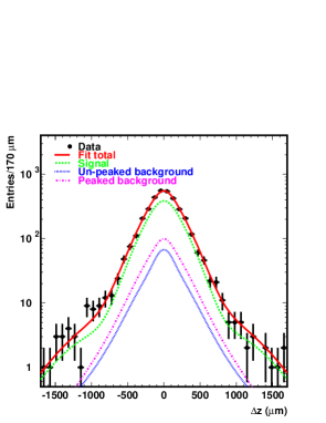
(a)

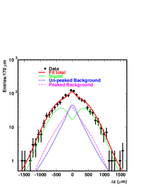
(b)

Figure 12: $\Delta z$ distributions for (a) opposite-flavor and (b) same-flavor events in data. The curve from the fit and the contributions of signal, unpeaked and peaked backgrounds are overlaid.

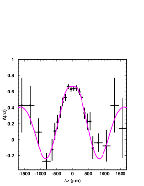
Figure 13: Distribution of the asymmetry, $A(\Delta z)$, as a function of $\Delta z$ for data with the fit curve overlaid.

Using the parameters determined above, $\Delta m_{d}$ is extracted from the fit. We find

$$\Delta m_{d}=(0.509\pm 0.017~{}({\rm stat}))~{}{\rm ps^{-1}}.$$ (13)

In Fig. 12 we show the $\Delta z$ distributions for SF and OF data together with the curves from the fit. To display the charge asymmetry (see Fig. 13) between SF and OF events, we use

$$A(\Delta z) \equiv {{\rm N^{OF}}(\Delta z)-{\rm N^{SF}}(\Delta z)\over{\rm N^{OF}}(\Delta z)+{\rm N^{SF}}(\Delta z)}~{},$$ (14)

where ${\rm N}(\Delta z)$ is the yield of the signal candidates as a function of $\Delta z$.

VI VALIDATION CHECK

We also perform a series of fits to signal Monte Carlo using the same procedure used in the analysis of the data. We generate four signal MC samples with different $\Delta m_{d}$ values. Table 1 summarizes the fitting results and shows the consistency between the input and extracted $\Delta m_{d}$. We conclude there is no significant fit bias.

Table 1: Summary of signal MC bias test.

$\Delta m_{d}~{}({\rm ps^{-1}})$ for MC generation	$\Delta m_{d}\rm~{}(ps^{-1})$ from fit yields
0.442	$0.448\pm 0.011$
0.472	$0.470\pm 0.012$
0.502	$0.492\pm 0.011$
0.532	$0.537\pm 0.012$

We also check for run dependence of the $\Delta m_{d}$ extraction. The value of $\Delta m_{d}$ is shown for four different experimental data taking periods (referred to as experiments 7, 9, 11, 13). The results are shown in Fig. 14(a).

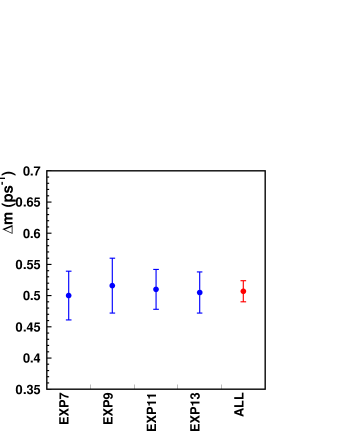
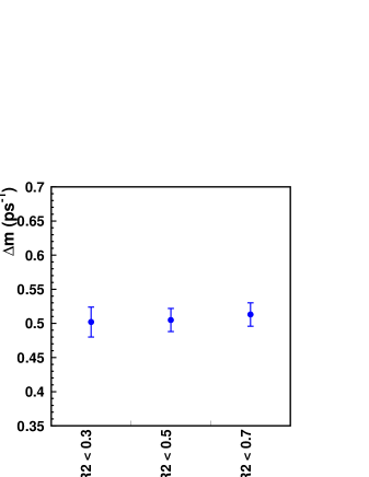
(a)                                                                 (b)

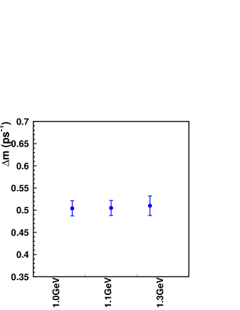
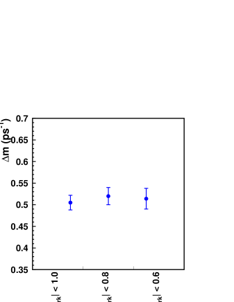
(c)                                                                 (d)

Figure 14: $\Delta m_{d}$ as function of (a) experiment number, (b) $R_{2}$ cut value, (c) cut on the lepton momentum in the CM frame, (d) lepton fiducial angle requirement.

To check the dependence of the $\Delta m_{d}$ fitting on the continuum background level, we also calculate $\Delta m_{d}$ as a function of the cut on the normalized second Fox-Wolfram moment foxwolfram $R_{2}=H_{2}/H_{0}$. The results are shown in Fig. 14(b).

We have also examined the variation of the fit results as the values of the cuts on the lepton momentum $p^{*}_{l}$ in the CM frame and the fiducial angle requirement for the lepton and $\pi_{f}$. The results are shown in Figs 14(c), (d). We find that all the variations are consistent with statistical fluctuations.

Furthermore, we performed fits separately for SF and OF events. Table 2 shows the fit results for SF events and OF events, respectively.

Table 2: Summary of $\Delta m_{d}$ fit results for SF (OF) events. Only statistical errors are shown.

Sample	Events	$\Delta m_{d}\rm~{}(ps^{-1})$
SF	1213	$\Delta m_{d}=0.511\pm 0.035$
OF	3686	$\Delta m_{d}=0.504\pm 0.019$

We also fit $e$ tagged events and $\mu$ tagged events separately (see Table 3).

Table 3: Summary of $\Delta m_{d}$ fit results for $e$ and $\mu$ tagged events. Only statistical errors are shown.

Sample	Events	$\Delta m_{d}\rm~{}(ps^{-1})$
$e$ tagged	2324	$\Delta m_{d}=0.510\pm 0.025$
$\mu$ tagged	2575	$\Delta m_{d}=0.503\pm 0.024$

To check the sensitivity of the result to tails of the vertex resolution function, we vary the $\Delta z$ range of the fit. The results are shown in Table 4 and are consistent with the primary result.

Table 4: Summary of $\Delta m_{d}$ fit results for different $\Delta z$ window. Only statistical errors are shown.

$\max(|\Delta z|)~{}(\rm\mu m)$	$\Delta m_{d}\rm~{}(ps^{-1})$
1700	$0.509\pm 0.017$
1275	$0.507\pm 0.017$
875	$0.511\pm 0.019$
425	$0.520\pm 0.024$

VII Systematic Uncertainties

Various possible sources of systematic uncertainties were investigated. In Table 5, we list the contributions to the systematic errors in $\Delta m_{d}$ that were estimated by varying the relevant parameters by one standard deviation.

Table 5: Contributions to the systematic error.

Source	Errors $\rm(ps^{-1})$
Background fraction	$\pm 0.014$
Signal resolution function	$\pm 0.012$
Background shape	$\pm 0.005$
$B^{0}$ lifetime $\rm(1.548\pm 0.032~{}ps)$	$\pm 0.005$
Detector resolution $\rm(50\pm 18~{}\mu m)$	$\pm 0.002$
Total	$\pm 0.020$

• $\mathbf{Background~{}fraction}$
  As described in Section IV.1, the background parts of the likelihood function are weighted by $f_{\rm bkg}$, $f_{\rm bkg}^{OF}$, $f_{\rm bkg}^{OF-unpeak}$ and $f_{\rm bkg}^{SF-unpeak}$ in Eq. (12), which are determined from a fit to the $D^{0}$ missing mass distribution in data. The corresponding systematic error, $\pm 0.014$, is estimated by varying the parameters of these background fractions by $\pm 1\sigma$.

• $\mathbf{Signal~{}resolution~{}function}$
  The fitted parameters of the $\Delta z$ distributions for $J/\psi\to l^{+}l^{-}$ events are varied according to the limited data statistics by $\pm 1\sigma$. The difference from the standard fit is taken as a measure of systematic error for each parameter. The corresponding uncertainty for each parameter is added in quadrature in order to estimate a systematic uncertainty in $\Delta m_{d}$ of $\pm 0.012\rm~{}ps^{-1}$.

• $\mathbf{Background~{}shape}$
  For both peaked and unpeaked backgrounds, the $\Delta z$ distributions are determined from a method described in Section IV.3. Varying all parameters by $\pm 1\sigma$, we take the differences, $\pm 0.004$, from the standard fit as the systematic error.

• $B^{0}$ $\mathbf{lifetime}$
  The value of the $B^{0}$ lifetime was varied according to the uncertainty of the PDG2000 PDG2000 value. Changes in $\Delta m_{d}$ of $\pm 0.005$ are observed.

• $\mathbf{Detector~{}resolution}$
  In Section IV.3, we mentioned that the MC background distributions are smeared to correct for the difference in the vertex resolution between the MC prediction and the data. The smearing function was a Gaussian with $\sigma=50~{}\mu$m. We varied the amount of smearing by its uncertainty ($18~{}\mu$m) christo and repeated the fit. We obtain a difference in $\Delta m_{d}$ of $\pm 0.002$

The total systematic error, obtained by summing all errors from the different sources in quadrature, is $\pm 0.020\rm~{}ps^{-1}$.

VIII CONCLUSION

Using 29.1 $\rm fb^{-1}$ of data collected with the Belle detector at the $\Upsilon(4S)$, we have measured the $B^{0}-\overline{B}^{0}$ mixing frequency $\Delta m_{d}$ in $B^{0}(\overline{B}^{0})\to D^{*\mp}\pi^{\pm}$ decay with a partial reconstruction technique. The data were accumulated between January 2000 and July 2001.

The asymmetric $e^{+}e^{-}$ beam energies of the KEKB collider allows for the extraction of the time evolution of the $B$ meson wave function from precise measurements of the decay vertex positions. The data are separated into SF and OF samples. The $B^{0}$ decay vertex resolution for the signal was determined from the $\Delta z$ distribution of $J/\psi\to l^{+}l^{-}$ decays that occur in the same data sample. The backgrounds are divided into two components, peaked and unpeaked backgrounds. The $\Delta m_{d}$ value, obtained by simultaneously fitting the SF and OF time distributions, is

$$\Delta m_{d} = (0.509\pm 0.017(\rm stat)\pm 0.020(\rm syst))~{}ps^{-1}.$$

This is the first direct measurement of $\Delta m_{d}$ using the technique of partial reconstruction of $B^{0}(\overline{B}^{0})\to D^{*\mp}\pi^{\pm}$ decays. This measurement is statistically uncorrelated with all other reported experimental results for $\Delta m_{d}$. It is also almost systematically independent from all other measurements. The systematic uncertainty is dominated by the background fractions and the signal resolution function; all quantities are measured experimentally except for the peaked background. This measurement agrees with the world average value of $\Delta m_{d}=(0.472\pm 0.017)\rm~{}ps^{-1}$ PDG2000 , and serves as a validation of the technique that will be used in the future for the measurement of the $CP$ violation parameter $\sin(2\phi_{1}+\phi_{3})$ zyh .

We wish to thank the KEKB accelerator group for the excellent operation of the KEKB accelerator. We acknowledge support from the Ministry of Education, Culture, Sports, Science, and Technology of Japan and the Japan Society for the Promotion of Science; the Australian Research Council and the Australian Department of Industry, Science and Resources; the National Science Foundation of China under contract No. 10175071; the Department of Science and Technology of India; the BK21 program of the Ministry of Education of Korea and the CHEP SRC program of the Korea Science and Engineering Foundation; the Polish State Committee for Scientific Research under contract No. 2P03B 17017; the Ministry of Science and Technology of the Russian Federation; the Ministry of Education, Science and Sport of Slovenia; the National Science Council and the Ministry of Education of Taiwan; and the U.S. Department of Energy.

Appendix A Background PDFs

For the background, the PDFs of OF and SF events are parameterized by

$$F^{\rm OF}_{\rm bkg}(\Delta t) = \int^{\infty}_{-\infty}(f_{\rm bkg}^{\rm OF-unpeak}{\rm P}_{\rm bkg}^{\rm OF-unpeak}(\Delta t^{\prime})$$ (15)

$$~{}~{}~{}~{}~{}\times R_{\rm bkg}^{\rm unpeak}(\Delta t-\Delta t^{\prime})$$

$$~{}~{}~{}+(1-f_{\rm bkg}^{\rm OF-unpeak}){\rm P}_{\rm bkg}^{\rm OF-peak}(\Delta t^{\prime})$$

$$~{}~{}~{}~{}~{}\times R_{\rm bkg}^{\rm peak}(\Delta t-\Delta t^{\prime}))d\Delta t^{\prime}~{},$$

$$F^{\rm SF}_{\rm bkg}(\Delta t) = \int^{\infty}_{-\infty}(f_{\rm bkg}^{\rm SF-unpeak}{\rm P}_{\rm bkg}^{\rm SF-unpeak}(\Delta t^{\prime})$$ (16)

$$~{}~{}~{}~{}~{}\times R_{\rm bkg}^{\rm unpeak}(\Delta t-\Delta t^{\prime})$$

$$~{}~{}~{}+(1-f_{\rm bkg}^{\rm SF-unpeak}){\rm P}_{\rm bkg}^{\rm SF-peak}(\Delta t^{\prime})$$

$$~{}~{}~{}~{}~{}\times R_{\rm bkg}^{\rm peak}(\Delta t-\Delta t^{\prime}))d\Delta t^{\prime}~{}.$$

Here, $f_{\rm bkg}^{\rm SF-unpeak}\equiv N_{\rm bkg}^{\rm SF-unpeak}/N_{\rm bkg}^{\rm SF}$ and $f_{\rm bkg}^{\rm OF-unpeak}\equiv N_{\rm bkg}^{\rm OF-unpeak}/N_{\rm bkg}^{\rm OF}$ are the fractions of unpeaked background in the SF and OF events. $N$ is the number of events, the subscripts $\rm bkg$ and $\rm sig$ denote the background and signal components. $R_{\rm bkg}^{\rm peak}(\Delta t)$ and $R_{\rm bkg}^{\rm unpeak}(\Delta t)$ are resolution functions for peaked and unpeaked background and are parameterized by triple-Gaussian distributions, which have the same form as the signal resolution function $R_{\rm sig}(\Delta t)$ in Eq. (11). In the fit, we use the signal resolution function for $R_{\rm bkg}^{\rm unpeak}(\Delta t)$. The peaked background resolution function $R_{\rm bkg}^{\rm peak}(\Delta t)$, described in Section IV.2, is determined from $J/\psi\to l^{+}l^{-}$ decays in MC with additional smearing.

In the unpeaked background PDF, ${\rm P}_{\rm bkg}^{\rm OF-unpeak}(\Delta t)$ and ${\rm P}_{\rm bkg}^{\rm SF-unpeak}(\Delta t)$ are defined by

$${\rm P}_{\rm bkg}^{\rm OF-unpeak}(\Delta t) = f_{0}^{\rm OF-unpeak}\delta(\Delta t)$$ (17)

$$\hskip-14.22636pt+(1-f_{0}^{\rm OF-unpeak}){1\over{2\tau_{\rm bkg}}}{e^{-{|\Delta t|\over\tau_{\rm bkg}}}}~{},$$

$${\rm P}_{\rm bkg}^{\rm SF-unpeak}(\Delta t) = f_{0}^{\rm SF-unpeak}\delta(\Delta t)$$ (18)

$$\hskip-14.22636pt+(1-f_{0}^{\rm SF-unpeak}){1\over{2\tau_{\rm bkg}}}{e^{-{|\Delta t|\over\tau_{\rm bkg}}}}~{}.$$

In the peaked background PDF, ${\rm P}_{\rm bkg}^{\rm OF-peak}(\Delta t)$ and ${\rm P}_{\rm bkg}^{\rm SF-peak}(\Delta t)$ are defined by

$${\rm P}_{\rm bkg}^{\rm OF-peak}(\Delta t) = f_{0}^{\rm OF-peak}\delta(\Delta t)$$ (19)

$$\hskip-39.83385pt+(1-f_{0}^{\rm OF-peak})(1-f_{1}^{\rm OF-peak}){1\over{2\tau_{\rm bkg}}}{e^{-{|\Delta t|\over\tau_{\rm bkg}}}}$$

$$\hskip-39.83385pt+(1-f_{0}^{\rm OF-peak})f_{1}^{\rm OF-peak}{\frac{1+\Delta m_{d}^{2}\tau_{\rm bkg}^{2}}{4\tau_{\rm bkg}+2\Delta m_{d}^{2}\tau_{\rm bkg}^{3}}}$$

$$\hskip-22.76219pt\times~{}{e^{-{|\Delta t|\over\tau_{\rm bkg}}}\left[1+\cos(\Delta m_{d}\Delta t)\right]}~{},$$

$${\rm P}_{\rm bkg}^{\rm SF-peak}(\Delta t) = f_{0}^{\rm SF-peak}\delta(\Delta t)$$ (20)

$$\hskip-39.83385pt+(1-f_{0}^{\rm SF-peak})(1-f_{1}^{\rm SF-peak}){1\over{2\tau_{\rm bkg}}}{e^{-{|\Delta t|\over\tau_{\rm bkg}}}}$$

$$\hskip-39.83385pt+(1-f_{0}^{\rm SF-peak})f_{1}^{\rm SF-peak}{\frac{1+\Delta m_{d}^{2}\tau_{\rm bkg}^{2}}{2\Delta m_{d}^{2}\tau_{\rm bkg}^{3}}}$$

$$\hskip-22.76219pt\times~{}{e^{-{|\Delta t|\over\tau_{\rm bkg}}}\left[1-\cos(\Delta m_{d}\Delta t)\right]}~{}.$$

In the above equations, $f_{0}$ is the prompt lifetime fraction and $(1-f_{0})f_{1}$ is the mixing fraction. $\tau_{\rm bkg}$ is the lifetime of the background component that does not originate from a prompt source. $\Delta m_{d}$ contributes to the peaked background since the peaked background is dominated by $B^{0}$ decays [20]. Thus, mixing terms are included in the PDFs for the peaked background. In the unpeaked background expression, we set the mixing term to zero since a parameterization without mixing reproduces the data well.

References

[1]
I. I. Bigi and A. I. Sanda.
“ Violation”.
Cambridge University Press, Cambridge, 2000.
[2]
A. J. Buras et al., Nucl. Phys. B 347, 491 (1990).
[3]
T. Inami and C. S. Lim, Prog. Theor. Phys. 65, 297 and 1772 (1981); A. J.
Buras, Phys. Rev. Lett. 46, 1354 (1981).
[4]
J. F. Donoghue, E. Golowich and B. R. Holstein. “Dynamics of the Standard
Model”. Cambridge University Press, Cambridge, 1992.
[5]
I. Dunietz and J. L. Rosner, Phys. Rev. D 34, 1404 (1986); I. Dunietz,
Phys. Lett. B 427, 179-182 (1998).
[6]
S. Kurokawa et al., KEK Preprint 2001-157 (2001), to appear in Nucl.
Instr. and Meth. A.
[7]
A. Abashian et al. (Belle Collaboration), Nucl. Instr. and Meth. A479, 117 (2002).
[8]
G. Alimonti et al., Nucl. Instr. and Meth. A453, 71 (2000).
[9]
H. Hirano et al., Nucl. Instr. and Meth. A455, 294 (2000);
M. Akatsu et al., Nucl. Instr. and Meth. A454, 322 (2000).
[10]
H. Kichimi et al., Nucl. Instr. and Meth. A453, 315 (2000).
[11]
T. Iijima et al., Nucl. Instr. and Meth. A453, 321 (2000).
[12]
H. Ikeda et al., Nucl. Instr. and Meth. A441, 401 (2000).
[13]
K. Hanagaki et al., submitted to Nucl. Instr. and Meth., hep-ex/0108044.
[14]
A.Abashian et al., Nucl. Instr. and Meth. A449, 112 (2000).
[15]
The QQ meson decay event generator was developed by
the CLEO Collaboration. See the following URL:
http://www.lns.cornell.edu/public/CLEO/soft/QQ.
[16]
CERN Program Library Long Writeup W5013, CERN, 1993.
[17]
K. Abe et al. (Belle Collaboration), Phys. Rev. D 64, 072001
(2001).
[18]
R. Giles et al. (CLEO Collaboration), Phys. Rev. D 30, 2279 (1984);
G. Brandenburg et al. (CLEO Collaboration), Phys. Rev. Lett. 80,
2762 (1998); B. H. Behrens et al. (CLEO Collaboration), Phys. Lett. B
490, 36-44 (2000).
[19]
D.E. Groom et al. Particle Data Group, Eur. Phys. J. C15, 1 (2000).
[20]
Yangheng Zheng, PhD dissertation, University of Hawaii at Manoa, Department of
Physics, 2002.
[21]
M. S. Alam et al. (CLEO Collaboration), Phys. Rev. D 50, 43-68
(1994).
[22]
T. Skwarnicki, PhD dissertation, Institute for Nuclear Physics, Krakow 1986;
DESY Internal Report, DESY F31-86-02 (1986).
[23]
G. Fox and S. Wolfram, Phys. Rev. Lett 41, 1581 (1978).
[24]
Christos Leonidopoulos, PhD dissertation, Princeton University, Department of
Physics, 2000.