The Discovery of Neutrino Masses

Abstract

The recent observation of neutrino oscillations with atmospheric and solar neutrinos, implying that neutrinos are not massless, is a discovery of paramount importance for particle physics and particle astrophysics. This invited lecture discusses — hopefully in a way understandable also for the non-expert — the physics background and the results mainly from the two most relevant experiments, Super-Kamiokande and SNO. It also addresses the implications for possible neutrino mass spectra. We restrict the discussion to three neutrino flavours ($\nu_{e},\nu_{\mu},\nu_{\tau}$), not mentioning a possible sterile neutrino.

1 Introduction

Until recently one of the fundamental questions in particle physics has been as to whether neutrinos have a mass ($m_{\nu}>0$, massive neutrinos) or are exactly massless (like the photon). This question is directly related to the more general question whether there is new physics beyond the Standard Model (SM): In the minimal SM, neutrinos have fixed helicity, always $H(\nu)=-1$ and $H(\overline{\nu})=+1$. This implies $m_{\nu}=0$, since only massless particles can be eigenstates of the helicity operator. $m_{\nu}>0$ would therefore transcend the simple SM. Furthermore, if $m_{\nu}$ is in the order of 1 - 10 eV, the relic neutrinos from the Big Bang ($n_{\nu}\approx 340/{\rm cm}^{3}$) would noticeably contribute to the dark matter in the universe.

Direct kinematic measurements of neutrino masses, using suitable decays, have so far yielded only rather loose upper limits, the present best values being [1]

$$\begin{array}[]{lll}m(\nu_{e})<3\>{\rm eV}&&({\rm from\>tritium}\>\beta\>{\rm decay})\\[4.30554pt] m(\nu_{\mu})<190\>{\rm keV}&(90$\%${\rm CL})&({\rm from}\>\pi^{+}\>{\rm decay})\\[4.30554pt] m(\nu_{\tau})<18.2\>{\rm MeV}&(95$\%${\rm CL})&({\rm from}\>\tau\>{\rm decays}).\end{array}$$ (1)

Another and much more sensitive access to neutrino masses is provided by neutrino oscillations [2]. They allow, however, to measure only differences of masses squared, $\delta m^{2}_{ij}\equiv m^{2}_{i}-m^{2}_{j}$, rather than masses directly. For completeness we summarize briefly the most relevant formulae for neutrino oscillations in the simplest case, namely in the vacuum and for only two flavours ($\nu_{a},\nu_{b}$), e.g. ($\nu_{e},\nu_{\mu}$) (two-flavour formalism). The generalization to three (or more) flavours is straight-forward in principle, but somewhat more involved in practice, unless special cases are considered, e.g. $m_{1}\approx m_{2}\ll m_{3}$ [2].

Figure 1: Scheme of a neutrino oscillation experiment.

The two flavour eigenstates ($\nu_{a},\nu_{b}$) are in general related to the two mass eigenstates $(\nu_{1},\nu_{2})$ with masses ($m_{1},m_{2}$) by a unitary transformation:

$$\left(\begin{array}[]{c}\nu_{a}\\ \nu_{b}\end{array}\right)=\left(\begin{array}[]{c@{\hspace{0.3cm}}c}\cos\theta\hfil\hskip 8.5359pt&\sin\theta\\ -\sin\theta\hfil\hskip 8.5359pt&\cos\theta\end{array}\right)\cdot\left(\begin{array}[]{c}\nu_{1}\\ \nu_{2}\end{array}\right)$$ (2)

where $\theta$ is the mixing angle. If $m_{1}\neq m_{2}$, the two mass eigenstates evolve differently in time, so that for $\theta\neq 0$ the given original linear superposition of $\nu_{1}$ and $\nu_{2}$ changes with time into a different superposition. This means that flavour transitions (oscillations) $\nu_{a}\to\nu_{b}$ and $\nu_{b}\to\nu_{a}$ can occur with certain time-dependent oscillatory probabilities. In other words (Fig. 1): If a neutrino is produced (or detected) at A as a flavour eigenstate $\nu_{a}$ (e.g. $\nu_{\mu}$ from $\pi^{+}\to\mu^{+}+\nu_{\mu}$), it is detected, after travelling a distance (baseline) $L$, at B with a probability $P(\nu_{a}\to\nu_{b})$ as flavour eigenstate $\nu_{b}$ (e.g. $\nu_{e}$ in $\nu_{e}n\to pe^{-}$). The transition probability $P(\nu_{a}\to\nu_{b})=P(\overline{\nu}_{a}\to\overline{\nu}_{b})=P(\nu_{b}\to\nu_{a})$ is given by

$$\left.\begin{array}[]{ll}P(\nu_{a}\to\nu_{b})&=\sin^{2}2\theta\cdot\sin^{2}\left({\displaystyle\frac{\delta m^{2}}{4}}\cdot{\displaystyle\frac{L}{E}}\right)\\[10.76385pt] &=\sin^{2}2\theta\cdot\sin^{2}\left(1.267{\displaystyle\frac{\delta m^{2}}{{\rm eV}^{2}}\cdot\frac{L/{\rm m}}{E/{\rm MeV}}}\right)\end{array}\right\}\begin{array}[]{l}{\rm for}\ \nu_{a}\neq\nu_{b}\\ ({\rm flavour~{}change}\\ \nu_{a}\to\nu_{b})\end{array}$$ (3)

$$P(\nu_{a}\to\nu_{a})=1-P(\nu_{a}\to\nu_{b})\ \ \ \ \ \mbox{(survival of $\nu_{a}$)}$$

where $\delta m^{2}=m^{2}_{2}-m^{2}_{1}$ and $E=$ neutrino energy. Thus the probability oscillates when varying $L/E$, with $\theta$ determining the amplitude $(\sin^{2}2\theta)$ and $\delta m^{2}$ the frequency of the oscillation. The smaller $\delta m^{2}$, the larger $L/E$ values are needed to see oscillations, i.e. significant deviations of $P(\nu_{a}\to\nu_{b})$ from zero and of $P(\nu_{a}\to\nu_{a})$ from unity. Notice the two necessary conditions for $\nu$ oscillations: (a) $m_{1}\neq m_{2}$ implying that not all neutrinos are massless, and (b) non-conservation of the lepton-flavour numbers.

In (3), $L$ and $E$ are the variables of an experiment, and $\theta$ and $\delta m^{2}$ the parameters (constants of Nature) to be determined. The original situation ($P(\nu_{a}\to\nu_{b})=\delta_{ab}$) is restored, if in (3) the distance $L$ is an integer multiple of the oscillation length $L_{\rm osc}$ which is given by

$$L_{\rm osc}=4\pi\dfrac{E}{\delta m^{2}}=2.48\dfrac{E/{\rm MeV}}{\delta m^{2}/{\rm eV}^{2}}\,{\rm m}.$$ (4)

The masses $m(\nu_{a})$ and $m(\nu_{b})$ of the flavour eigenstates are expectation values of the mass operator, i.e. linear combinations of $m_{1}$ and $m_{2}$:

$$\begin{array}[]{l}m(\nu_{a})=\cos^{2}\theta\cdot m_{1}+\sin^{2}\theta\cdot m_{2}\\[4.30554pt] m(\nu_{b})=\sin^{2}\theta\cdot m_{1}+\cos^{2}\theta\cdot m_{2}.\end{array}$$ (5)

2 Flavour change of atmospheric neutrinos

The most convincing evidence for a flavour change of atmospheric neutrinos was found in 1998 by Super-Kamiokande[3, 4], after first indications were observed by some earlier experiments (Kamiokande [5], IMB [6], Soudan 2 [7]).

Atmospheric neutrinos are created when a high-energy cosmic-ray proton (or nucleus) from outer space collides with a nucleus in the earth’s atmosphere, leading to an extensive air shower (EAS) by cascades of secondary interactions. Such a shower contains many $\pi^{\pm}$ (and $K^{\pm}$) mesons (part of) which decay according to

$$\begin{array}[]{ll@{\hspace{1cm}}ll}\pi^{+},K^{+}\rightarrow&\mu^{+}\nu_{\mu}\hfil\hskip 28.45274pt&\pi^{-},K^{-}\rightarrow&\mu^{-}\overline{\nu}_{\mu}\\ &\;\rule[2.15277pt]{0.4pt}{4.30554pt}\rightarrow e^{+}\nu_{e}\overline{\nu}_{\mu}\hfil\hskip 28.45274pt&&\;\rule[2.15277pt]{0.4pt}{4.30554pt}\rightarrow e^{-}\overline{\nu}_{e}\nu_{\mu}\,,\end{array}$$ (6)

yielding atmospheric neutrinos. From (6) one would expect in an underground neutrino detector a number ratio of

$$\frac{\mu}{e}\equiv\frac{\nu_{\mu}+\overline{\nu}_{\mu}}{\nu_{e}+\overline{\nu}_{e}}=2\,,$$ (7)

if all $\mu^{\pm}$ decayed before reaching the detector. This is the case only at rather low shower energies whereas with increasing energy more and more $\mu^{\pm}$ survive due to relativistic time dilation and may reach the detector as background (atmospheric $\mu$). Consequently the expected $\mu/e$ ratio rises above 2 (fewer and fewer $\nu_{e},\overline{\nu}_{e}$) with increasing $\nu$ energy. For quantitative predictions Monte Carlo (MC) simulations, which include also other (small) $\nu$ sources, have been performed, using measured $\mu$ fluxes as input, modelling the air showers in detail, and yielding the fluxes of the various neutrino species ($\nu_{e},\overline{\nu}_{e},\nu_{\mu},\overline{\nu}_{\mu}$) as a function of the $\nu$ energy [8].

Atmospheric neutrinos reaching the underground Super-K detector can be registered by neutrino reactions with nucleons inside the detector, the simplest and most frequent reactions being CC quasi-elastic scatterings:

$$({\rm a})\mbox{\hskip 8.5359pt}\begin{array}[]{l}\nu_{e}n\to pe^{-}\\ \overline{\nu}_{e}p\to ne^{+}\end{array}\mbox{\hskip 22.76228pt (b)\hskip 8.5359pt}\begin{array}[]{l}\nu_{\mu}n\to p\mu^{-}\\ \overline{\nu}_{\mu}p\to n\mu^{+}\,.\end{array}$$ (8)

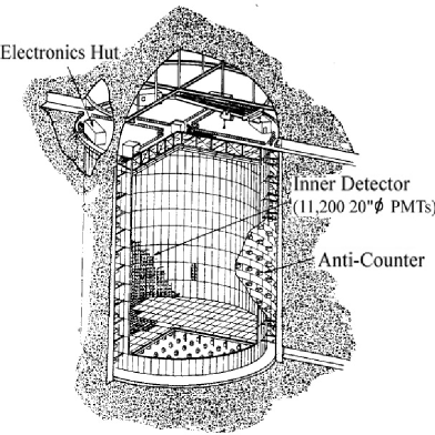
Figure 2: Schematic view of Super-Kamiokande [9].

Super-K (Fig. 2)[9] is a big water-Cherenkov detector in the Kamioka Mine (Japan) at a depth of $\sim$ 1000 m. It consists of 50 ktons (50 000 m³) of ultrapurified water in a cylindrical tank (diameter = 39 m, height = 41 m). The inner detector volume of 32 ktons is watched by 11 146 photomultiplier tubes (PMTs, diameter = 20^′′) mounted on the volume’s surface and providing a 40% surface coverage. The outer detector, which tags entering particles and exiting particles, is a 2.5 m thick water layer surrounding the inner volume and looked at by 1885 smaller PMTs (diameter = 8^′′). A high-velocity charged particle passing through the water produces a cone of Cherenkov light which is registered by the PMTs. The Cherenkov image of a particle starting and ending inside the inner detector is a ring, the image of a particle starting inside and leaving the inner detector is a disk. A distinction between an $e$-like event (8a) and a $\mu$-like event (8b) is possible (with an efficiency of $\mbox{$\stackrel{{\scriptstyle\scriptstyle>}}{{\scriptstyle\sim}}$}\ 98\%$) from the appearance of the image: an $e^{\pm}$ has an image with a diffuse, fuzzy boundary whereas the boundary of a $\mu^{\pm}$ image is sharp. The observed numbers of $\mu$-like and $e$-like events give directly the observed $\nu$-flux ratio $(\mu/e)_{\rm obs}$ (eq. 7) which is to be compared with the MC-predicted ratio $(\mu/e)_{\rm MC}$ (for no $\nu$ oscillations) by computing the double ratio

$$R=\frac{(\mu/e)_{\rm obs}}{(\mu/e)_{\rm MC}}\,.$$ (9)

Agreement between observation and expectation implies $R=1$.

The events are separated into fully contained events (FC, no track leaving the inner volume, $\langle E_{\nu}\rangle\sim 1\,{\rm GeV}$) and partially contained events (PC, one or more tracks leaving the inner volume, $\langle E_{\nu}\rangle\sim 10\,{\rm GeV}$). For FC events the visible energy $E_{\rm vis}$, which is obtained from the pulse heights in the PMTs, is close to the $\nu$ energy. With this in mind, the FC sample is subdivided into sub-GeV events ($E_{\rm vis}<1.33$ GeV) and multi-GeV events ($E_{\rm vis}>1.33$ GeV). In the multi-GeV range the $\nu$ direction can approximately be determined as the direction of the Cherenkov-light cone, since at higher energies the directions of the incoming $\nu$ and the outgoing charged lepton are close to each other.

Results on the double-ratio R. The first error is statistical, the second systematic (kty = kilotons $\cdot$ years). Super-K $R=0.652\pm 0.019\pm 0.051$ sub-GeV $(E_{\rm vis}<1.33\,{\rm GeV})$ (70.5 kty) $R=0.661\pm 0.034\pm 0.079$ multi-GeV $(E_{\rm vis}>1.33\,{\rm GeV})$ Soudan 2 (5.1 kty) $R=0.68\pm 0.11\pm 0.06$

Recent results on R from Super-K [4] and Soudan 2 [10] are given in Tab. 2. All three R values are significantly smaller than unity (“atmospheric neutrino anomaly”) which is due, as it turns out (see below), to a deficit of $\nu_{\mu},\overline{\nu}_{\mu}$ and not to an excess of $\nu_{e},\overline{\nu}_{e}$ in $(\mu/e)_{\rm obs}$. A natural explanation of this deficit is that some $\nu_{\mu},\overline{\nu}_{\mu}$ have oscillated into $(\nu_{e},\overline{\nu}_{e})$ or $(\nu_{\tau},\overline{\nu}_{\tau})$ according to (3) before reaching the detector.

This explanation has become evident, with essentially only $\nu_{\mu}\rightarrow\nu_{\tau}$ remaining (see below), by a study of the $\nu$ fluxes as a function of the zenith angle $\Theta$ between the vertical (zenith) and the $\nu$ direction. A $\nu$ with $\Theta\approx 0^{\circ}$ comes from above (down-going $\nu$) after travelling a distance of $L\ \mbox{$\stackrel{{\scriptstyle\scriptstyle<}}{{\scriptstyle\sim}}$}\ 20$ km (effective thickness of the atmosphere); a $\nu$ with $\Theta\approx 180^{\circ}$ reaches the detector from below (up-going $\nu$) after traversing the whole earth with $L\approx 13000$ km.

Figure 3: Zenith-angle distribution of (a) sub-GeV e-like, (b) multi-GeV e-like, (c) sub-GeV $\mu$-like, and (d) multi-GeV $\mu$-like + PC events. (The PC events turned out to be practically all $\nu_{\mu}$ events). The points show the data, the full histograms the MC predictions for no oscillations and the dotted histograms the best fit by $\nu_{\mu}\rightarrow\nu_{\tau}$ oscillations. From Super-K[4].

The zenith angular distributions (zenith angle of the charged lepton) as measured by Super-K[4] are shown in Fig. 3 for e-like and $\mu$-like events, in each event class separately for sub-GeV and multi-GeV events. The full histograms show the MC predictions for no oscillations. The e-like distributions (a) and (b) are both seen to be in good agreement with the predictions which implies that there is no $\nu_{e}$ excess and no noticeable $\nu_{\mu}\rightarrow\nu_{e}$ transition. The $\mu$-like distributions (c) and (d) on the other hand both show a $\nu_{\mu}$ deficit with respect to the predictions. For multi-GeV $\mu$-like events (d), for which the $\nu$ and $\mu$ directions are well correlated (see above), the deficit increases with increasing zenith angle, i.e. increasing flight distance L of the $\nu$ between production and detection; it is absent for down-going muons ($\Theta\approx 0^{\circ}$) and large for up-going muons ($\Theta>90^{\circ}$). For sub-GeV $\mu$-like events (c) the dependence of the deficit on $\Theta$ is much weaker, owing to the only weak correlation between the $\nu$ and $\mu$ directions.

In conclusion, all four distributions of Fig. 3 are compatible with the assumption, that part of the original $\nu_{\mu}$ change into $\nu_{\tau}$ (thus not affecting the e-like distributions), if their flight distance L is sufficiently long ($L\,\mbox{$\stackrel{{\scriptstyle\scriptstyle>}}{{\scriptstyle\sim}}$}\,L_{\rm osc}$).

This conclusion is supported by a Super-K measurement of the zenith angular distribution of up-going muons with $\Theta>90^{\circ}$ that enter the detector from outside [11, 4]. Because of their large zenith angle they cannot be atmospheric muons — those would not range so far into the earth —, but are rather produced in CC reactions by energetic up-going $\nu_{\mu},\overline{\nu}_{\mu}$ in the rock surrounding the detector. A clear deficit is observed for upward muons stopping in the detector ($\langle E_{\nu}\rangle\sim 10$ GeV) whereas it is much weaker for upward through-going muons ($\langle E_{\nu}\rangle\sim 100$ GeV). A deficit of atmospheric $\nu_{\mu},\overline{\nu}_{\mu}$ has also been observed by the MACRO collaboration[12] in the Gran Sasso Underground Laboratory in a similar measurement, their ratio of the numbers of observed to expected events being $\mu_{\rm obs}/\mu_{\rm exp}=0.72\pm 0.13$ (three errors added in quadrature) for upward through-going muons ($\langle E_{\nu}\rangle\sim 100$ GeV).

A two-flavour oscillation analysis, with $\sin^{2}2\theta$ and $\delta m^{2}$ as free parameters, has been carried out by the Super-K collaboration, using their data on (partially) contained events (Fig. 3) and including also their data on up-going muons. A good fit with $\chi^{2}/NDF=135/152$ has been obtained[4] for $\nu_{\mu}\leftrightarrow\nu_{\tau}$, the best-fit parameters being:

$$\delta m^{2}=3.2\cdot 10^{-3}\,{\rm eV}^{2}\,,\,\sin^{2}2\theta=1.$$ (10)

Figure 4: Regions (to the right of the curves) allowed at 68 %, 90 % and 99 % CL in the ($\sin^{2}2\theta,\delta m^{2}$) plane for $\nu_{\mu}\leftrightarrow\nu_{\tau}$ oscillations. From Super-K[4].

Fig. 4 shows the allowed regions with 68 %, 90 % and 99 % CL in the parameter plane. The best fit is also shown by the dotted histograms in Fig. 3, where excellent agreement with the data points is observed. From (4) and (10) one obtains an oscillation length of $L_{\rm osc}=775\,{\rm km}\cdot E/{\rm GeV}$. Thus, a flavour-change signal is not expected, because of $L\ll L_{\rm osc}$, (a) for neutrinos with $\Theta\approx 0^{\circ}$ (i.e. $L\,\mbox{$\stackrel{{\scriptstyle\scriptstyle<}}{{\scriptstyle\sim}}$}\,20$ km) and $E\,\mbox{$\stackrel{{\scriptstyle\scriptstyle>}}{{\scriptstyle\sim}}$}\,1$ GeV (Fig. 3d), and (b) for neutrinos producing upward through-going muons with $E\sim 100$ GeV (see above) so that $L_{\rm osc}\sim 80000$ km — much larger than the diameter of the earth.

No good fit could be obtained for $\nu_{\mu}\leftrightarrow\nu_{e}$ oscillations. In addition, $\overline{\nu}_{e}$ disappearance ($\overline{\nu}_{e}\rightarrow\overline{\nu}_{\rm X}$) has not been observed by two long-baseline reactor experiments (CHOOZ[13] and Palo Verde[14]) with $L\approx 1$ km and $\langle E\rangle\sim 3$ MeV, which rule out $\delta m^{2}>0.7\cdot 10^{-3}\,{\rm eV}^{2}$ for $\sin^{2}2\theta=1$, and $\sin^{2}2\theta>0.1$ for large $\delta m^{2}$.

In summary: Atmospheric neutrinos have yielded convincing evidence, mostly contributed by Super-K, that $\nu_{\mu}\leftrightarrow\nu_{\tau}$ oscillations take place with parameters given by Fig. 4 and Eq. (10). There is no other hypothesis around that can explain the data. One therefore has to conclude that not all neutrinos are massless.

3 Flavour change of solar neutrinos

Very exciting discoveries regarding neutrino masses have recently been made with solar neutrinos, in particular by the Sudbury Neutrino Observatory (SNO). Solar neutrinos[15] come from the fusion reaction

$$4p\to{\rm He}^{4}+2e^{+}+2\nu_{e}$$ (11)

inside the sun with a total energy release of 26.7 MeV after two $e^{+}e^{-}$ annihilations. The $\nu$ energy spectrum extends up to about 15 MeV with an average of $\langle E_{\nu}\rangle=0.59$ MeV. The total $\nu$ flux from the sun is $\phi_{\nu}=1.87\cdot 10^{38}$ s^-1 resulting in a flux density of $6.6\cdot 10^{10}\,{\rm cm}^{-2}\,{\rm s}^{-1}$ on earth.

Reaction (11) proceeds in various steps in the pp chain or CNO cycle, the three most relevant out of eight different $\nu_{e}$ sources being:

$$\begin{array}[]{l@{\ :\ \ }l@{\hspace{0.3cm}}l}pp&p+p\to D+e^{+}+\nu_{e}\hfil\hskip 8.5359pt&(E_{\nu}<0.42\ {\rm MeV},\,0.91)\\[4.30554pt] {\rm Be}^{7}&{\rm Be}^{7}+e^{-}\to{\rm Li}^{7}+\nu_{e}\hfil\hskip 8.5359pt&(E_{\nu}=0.86\ {\rm MeV},\,0.07)\\[4.30554pt] {\rm B}^{8}&{\rm B}^{8}\to{\rm Be}^{8}+e^{+}+\nu_{e}\hfil\hskip 8.5359pt&(E_{\nu}<14.6\ {\rm MeV},\,\sim 10^{-4}).\end{array}$$ (12)

The second number in each bracket gives the fraction of the total solar $\nu$ flux. Energy spectra of the $\nu_{e}$ fluxes from the various sources and rates for the various detection reactions have been predicted in the framework of the Standard Solar Model (SSM)[16, 17]. With respect to these predictions a $\nu_{e}$ deficit from the sun has been observed in the past by various experiments as listed in Tab. 3 (see ratios Result/SSM). These deficits, the well-known “solar neutrino problem”, could be explained by $\nu$ oscillations $\nu_{e}\to\nu_{X}$ into another flavour $X$ ($\nu_{e}$ disappearance) either inside the sun (matter oscillations, Mikheyev-Smirnov-Wolfenstein (MSW) effect[23]) or on their way from sun to earth (vacuum oscillations, $L\approx 1.5\cdot 10^{8}$ km), see below.

The five previous solar $\nu$ experiments and their results (adopting a recent compilation in Table 8 of Ref.[17]). The SSM is BP2000[17]. Threshold Result Experiment Reaction [MeV] (Result/SSM) Homestake[18] Cl³⁷$(\nu_{e},e^{-})$Ar³⁷ $E_{\nu}>0.814$ 2.56 $\pm$ 0.23 SNU (0.34 $\pm 0.06$) GALLEX + GNO[19] Ga⁷¹$(\nu_{e},e^{-})$Ge⁷¹ $E_{\nu}>0.233$ $74\pm 7$ SNU⁺ (0.58 $\pm$ 0.07) SAGE[20] Ga⁷¹$(\nu_{e},e^{-})$Ge⁷¹ $E_{\nu}>0.233$ 75 $\pm$ 8 SNU⁺ (0.59 $\pm$ 0.07) Kamiokande[21] $\nu e\to\nu e$ $E_{\nu}>7.5$ (2.80 $\pm$ 0.38) $\cdot 10^{6}$ cm^-2 s^-1 (0.55 $\pm$ 0.13) Super-Kamiokande[22] $\nu e\to\nu e$ $E_{\nu}>5.5$ $\left(2.40{+0.09\atop-0.08}\right)\cdot 10^{6}$ cm^-2 s^-1 (0.48 $\pm$ 0.09)

1 SNU (Solar Neutrino Unit) = 1 $\nu_{e}$ capture per 10³⁶ target nuclei per sec
⁺ The latest values (Neutrino 2002) are $71\pm 6$ for GALLEX + GNO and $71^{+7}_{-8}$ for SAGE.

Figure 5: Schematic drawing of the SNO detector.

We now discuss the new results from SNO[24, 25]. The SNO detector[26] (Fig. 5) is a water-Cherenkov detector, sited 2040 m underground in an active nickel mine near Sudbury (Canada). It comprises 1000 tons of ultra-pure heavy water (D₂O) in a spherical transparent acrylic vessel (12 m diameter) serving as a target and Cherenkov radiator. Cherenkov photons produced by electrons in the sphere are detected by 9456 20 cm-photomultiplier tubes (PMTs) which are mounted on a stainless steel structure (17.8 m diameter) around the acrylic vessel. The vessel is immersed in ultra-pure light water (H₂O) providing a shield against radioactivity from the surrounding materials (PMTs, rock).

SNO detects the following three reactions induced by solar B⁸-neutrinos above an electron threshold of 5 MeV for the SNO analysis (d = deuteron):

$$\begin{array}[]{lclll}\nu_{e}+{\rm d}&\rightarrow&\mbox{ \boldmath$e^{-}$}+p+p&{\rm(CC)}&\hskip 8.53581ptE_{\rm thresh}=1.44\,{\rm MeV}\\ \nu_{X}+{\rm d}&\rightarrow&\nu_{X}+p+n&{\rm(NC)}&\hskip 8.53581ptE_{\rm thresh}=2.23\,{\rm MeV}\\ &&\lx@intercol n+{\rm d}\rightarrow{{\rm H}^{3}}+\gamma\,(6.25\,{\rm MeV}),\,\gamma+e^{-}\rightarrow\gamma+\mbox{\boldmath$e^{-}$}\hfil\lx@intercol\\ \nu_{X}+e^{-}&\rightarrow&\nu_{X}+\mbox{\boldmath$e^{-}$}&{\rm(ES)}\end{array}$$ (13)

where the Cherenkov-detected electron is indicated by bold printing. The charged-current (cc) reaction (CC) can be induced only by $\nu_{e}$ whereas the neutral-current (nc) reaction (NC) is sensitive, with equal cross sections, to all three neutrino flavours $\nu_{e},\,\nu_{\mu},\,\nu_{\tau}$. Also elastic $\nu_{e}$-scattering (ES) is sensitive to all flavours, but with a cross section relation

$$\sigma(\nu_{\mu}e)=\sigma(\nu_{\tau}e)=\varepsilon\sigma(\nu_{e}e)$$ (14)

where $\varepsilon$ = 0.154 above 5 MeV according to the electroweak theory. ($\varepsilon\neq 1$ since $\nu_{\mu,\tau}e$ scattering goes only via nc, whereas $\nu_{e}e$ scattering has in addition to nc also a contribution from cc).

Data taking by SNO began in summer 1999. For each event (electron) the effective kinetic energy T, the angle $\Theta_{\rm sun}$ with respect to the direction from the sun, and the distance (radius) R from the detector center were measured. The principle of the analysis goes as follows: The three measured distributions $N(x)_{\rm meas}$ of $x=T,\,\Theta_{\rm sun},\,R^{3}$ from 2928 events with $5<T<20$ MeV can be fitted by three linear combinations

$$N(x)=N_{\rm CC}\cdot w_{\rm CC}(x)+N_{\rm NC}\cdot w_{\rm NC}(x)+N_{\rm ES}\cdot w_{\rm ES}(x)+N_{\rm BG}\cdot w_{\rm BG}(x)$$ (15)

where $w_{\rm i}(x)$ are characteristic probability density functions known from Monte Carlo simulations (e.g. $w_{\rm ES}(\cos\Theta_{\rm sun}$) is strongly peaked in the direction from the sun, i.e. towards $\cos\Theta_{\rm sun}=1$), and the parameters $N_{\rm i}$ are the numbers of events in the three categories (13) to be determined from the fit. $N_{\rm BG}$ for the background was fixed as determined from a background calibration. A good extended maximum likelihood fit to the measured distributions was obtained yielding (errors symmetrized):

$$N_{\rm CC}=1967.7\pm 61.4,\,N_{\rm NC}=576.5\pm 49.2,\,N_{\rm ES}=263.6\pm 26.0.$$ (16)

From each of these event numbers $N_{\rm i}$ a B⁸-neutrino flux $\Phi^{\rm SNO}_{\rm i}$ was determined, using the known cross sections for reactions (13) and the SSM B⁸-$\nu$ spectrum. The exciting result (in units of $10^{6}$ cm^-2 s^-1) is[24] (statistical and systematic errors added in quadrature):

$$\Phi^{\rm SNO}_{\rm CC}=1.76\pm 0.10,\,\Phi^{\rm SNO}_{\rm NC}=5.09\pm 0.62,\,\Phi^{\rm SNO}_{\rm ES}=2.39\pm 0.26$$ (17)

where $\Phi^{\rm SNO}_{\rm ES}$ has been computed using $\sigma(\nu_{e}e)$, i.e. assuming no $\nu_{e}$-oscillations. $\Phi^{\rm SNO}_{\rm ES}$ agrees nicely with the Super-K result[27] $\Phi^{\rm SK}_{\rm ES}=2.32\pm 0.09$, computed with the same assumption.

$\Phi^{\rm SNO}_{\rm CC}$ is the genuine $\nu_{e}$ flux $\Phi(\nu_{e})$ arriving at earth. For the case that the $\nu_{e}$ created in the sun arrived at earth all as $\nu_{e}$, i.e. there were no $\nu_{e}$ oscillations, one would expect $\Phi_{\rm CC}=\Phi_{\rm NC}=\Phi_{\rm ES}$. The SNO result (17) shows that this is obviously not the case, i.e. that there is significant direct evidence for a non-$\nu_{e}$ component in the solar $\nu$ flux arriving at earth.

The two fluxes $\Phi(\nu_{e})$ and $\Phi(\nu_{\mu\tau})$ (= $\nu_{\mu}+\nu_{\tau}$ flux) and the total $\nu$ flux $\Phi_{\rm tot}$ have been determined from (17) by a fit using the three relations

$$\begin{array}[]{lcl}\Phi_{\rm CC}&=&\Phi(\nu_{e})\\ \Phi_{\rm NC}&=&\Phi(\nu_{e})+\Phi(\nu_{\mu\tau})=\Phi_{\rm tot}\\ \Phi_{\rm ES}&=&\Phi(\nu_{e})+\varepsilon\Phi(\nu_{\mu\tau})\,{\rm with}\;\varepsilon=0.154\end{array}$$ (18)

with the result

$$\Phi(\nu_{e})=1.76\pm 0.10\,\,\,{\rm and}\,\,\,\Phi(\nu_{\mu\tau})=3.41\pm 0.65.$$ (19)

Notice that $\Phi(\nu_{\mu\tau})$ is different from zero by 5.3 $\sigma$ which is clear evidence for some ($\sim$ 66 %) of the original $\nu_{e}$ having changed their flavour. Furthermore, the measured value (17) $\Phi^{\rm SNO}_{\rm NC}=\Phi^{\rm SNO}_{\rm tot}=5.09\pm 0.62$ (or the value $\Phi_{\rm tot}=\Phi(\nu_{e})+\Phi(\nu_{\mu\tau})=5.17\pm 0.66$ from the fit result(19)) agrees nicely (within the large errors) with the SSM value[17] $\Phi^{\rm SSM}_{\rm tot}=5.05^{+1.01}_{-0.81}$; this agreement is a triumph of the Standard Solar Model.

The SNO analysis is summarized in the $\left[\Phi(\nu_{e}),\,\Phi(\nu_{\mu\tau})\right]$ plane, Fig. 6. The four bands show the straight-line relations (with their errors):

$$\begin{array}[]{lcl}\Phi^{\rm SNO}_{\rm CC}&=&\Phi(\nu_{e})=1.76\pm 0.10\\[4.30554pt] \Phi^{\rm SNO}_{\rm ES}&=&\Phi(\nu_{e})+0.154\cdot\Phi(\nu_{\mu\tau})=2.39\pm 0.26\\[4.30554pt] \Phi^{\rm SNO}_{\rm NC}&=&\Phi(\nu_{e})+\Phi(\nu_{\mu\tau})=5.09\pm 0.62\\[4.30554pt] \Phi^{\rm SSM}_{\rm tot}&=&\Phi(\nu_{e})+\Phi(\nu_{\mu\tau})=5.05^{+1.01}_{-0.81}.\end{array}$$ (20)

Full consistency of the three measurements (17) amongst themselves and with the SSM is observed, the four bands having a common intersection.

Best-fit values for the five solutions from Ref. 29 Solution $\delta m^{2}$(eV²) $\tan^{2}\theta$ $\chi^{2}_{\rm min}$ LMA $\Big{\}}$ MSW $4.2\times 10^{-5}$ $2.6\times 10^{-1}$ 29.0 SMA $5.2\times 10^{-6}$ $5.5\times 10^{-4}$ 31.1 LOW $7.6\times 10^{-8}$ $7.2\times 10^{-1}$ 36.0 Just So² $5.5\times 10^{-12}$ $1.0\times 10^{0}$ 36.1 VAC $1.4\times 10^{-10}$ $3.8\times 10^{-1}$ 37.5

A two-flavour oscillation analysis $(\nu_{e}\leftrightarrow\nu_{\mu}\,\,{\rm or}\,\,\nu_{\tau})$ has been carried out by the SNO collaboration[25]. Prior to SNO several global oscillation analyses were performed using all available solar neutrino data, including the Super-K measurements of the electron energy spectrum and of the day-night asymmetry (which could originate from a regeneration of $\nu_{e}$ in the earth at night)[27, 28]. Five allowed regions (e.g. at 3$\sigma$, i.e. 99.7 % CL) in the ($\tan^{2}\theta,\,\delta m^{2}$) plane were identified, their best-fit values e.g. from Ref.[29] being listed in Table 3. These solutions, apart from Just So², were also found by SNO[25] when only using their own data (measured day and night energy spectra), Fig. 7a. When including also the data from the previous experiments as well as SSM predictions in their analysis, only the large-mixing-angle (LMA) MSW solution is strongly favoured (Fig. 7b), the best-fit values being

$$\delta m^{2}=5.0\cdot 10^{-5}\,{\rm eV}^{2},\,\tan^{2}\theta=0.34\;(\theta=30^{\circ}).$$ (21)

The elimination of most of the other solutions is based on the Super-K measurements of the energy spectra during the day and during the night[28, 30]. However, the issue seems not completely settled yet[31].

Figure 6: Fluxes of B⁸-neutrinos as determined by SNO[24]. The bands show the flux $\Phi_{\mu\tau}$ of ($\nu_{\mu}+\nu_{\tau})$ vs. the flux $\Phi_{e}$ of $\nu_{e}$ according to each of the three experimental relations and the SSM relation[17] in (20). The intercepts of these bands with the axes represent the $\pm 1\sigma$ errors. The point in the intersection of the bands indicates the best-fit values (19). The ellipses around this point represent the 68 %, 95 % and 99 % joint probability contours for $\Phi_{e},\Phi_{\mu\tau}$. From Ref. [24].

Figure 7: Regions allowed at the indicated confidence levels in the parameter plane as determined from a $\chi^{2}$ fit (a) to the SNO day and night energy spectra alone, and (b) with the addition of data from the other solar experiments and of SSM predictions [17]. The star in the LMA solution indicates the best fit (21). From SNO [25].

In summary: Solar neutrinos have yielded strong evidence vor $\nu_{e}\leftrightarrow\nu_{X}\,(X=\mu,\,\tau)$ oscillations. In particular the recent SNO measurements show explicitly that the solar $\nu$ flux arriving at earth has a non-$\nu_{e}$ component. These measurements and their good agreement with the SSM have solved the long standing solar neutrino problem; they are evidence, in addition to the results from atmospheric neutrinos, for neutrinos having mass.

4 Possible neutrino mass schemes

With two independent $\delta m^{2}$ values, namely (10) $\delta m^{2}_{\rm atm}\approx 3.2\cdot 10^{-3}$ eV² and (21) $\delta m^{2}_{\rm sol}\approx 5.0\cdot 10^{-5}$ eV² one needs three neutrino mass eigenstates $\nu_{\rm i}=\nu_{1},\nu_{2},\nu_{3}$ with masses $m_{1},m_{2},m_{3}$ obeying the relation $\delta m^{2}_{21}+\delta m^{2}_{32}+\delta m^{2}_{13}=0$ where $\delta m^{2}_{\rm ij}=m^{2}_{\rm i}-m^{2}_{\rm j}$. The neutrino flavour eigenstates $\nu_{\alpha}=\nu_{e},\nu_{\mu},\nu_{\tau}$ are then linear combinations of the $\nu_{\rm i}$ and vice versa, $\nu_{\alpha}=\sum_{\rm i}{U_{\alpha\rm i}\nu_{\rm i}}$, in analogy to (2).

Figure 8: Schematic drawing of the normal and inverted hierarchical mass spectrum of the 3 neutrino mass eigenstates $\nu_{\rm i}\,(i=1,2,3)$. The shadings show the admixtures $\left|U_{\rm ei}\right|^{2}$ (white), $\left|U_{\mu{\rm i}}\right|^{2}$ (grey) and $\left|U_{\tau{\rm i}}\right|^{2}$ (black) of the 3 flavour eigenstates $\nu_{e},\nu_{\mu}$ and $\nu_{\tau}$, respectively. Adapted from Ref. [32].

The absolute neutrino mass scale is still unknown, since a direct measurement of a neutrino mass has not yet been accomplished. Several possible mass schemes have been proposed in the literature. The two main categories are:

• A hierarchical mass spectrum, e.g. $m_{1}\ll m_{2}\ll m_{3}$. In this case the hierarchy may be normal or inverted, as shown in Fig. 8. If e.g. for the normal hierarchy one assumes $m_{1}\approx 0$, then

  $$\begin{array}[]{lclclclc}m_{2}&\approx&\sqrt{\delta m^{2}_{21}}&\approx&\sqrt{\delta m^{2}_{\rm sol}}\approx\sqrt{5\cdot 10^{-5}}\,\,{\rm eV}&\approx&7\cdot 10^{-3}\,\,{\rm eV},\\[4.30554pt] m_{3}&\approx&\sqrt{\delta m^{2}_{31}}&\approx&\sqrt{\delta m^{2}_{\rm atm}}\approx\sqrt{3.2\cdot 10^{-3}}\,\,{\rm eV}&\approx&6\cdot 10^{-2}\,\,{\rm eV}.\end{array}$$ (22)

• A democratic (nearly degenerate) mass spectrum with $m_{1}\approx m_{2}\approx m_{3}\gg\sqrt{\delta m^{2}}$. In this case almost any $m_{\nu}$ value below $\sim 3$ eV (upper limit of $m(\nu_{e})$, eq. (1)) is possible. In particular, with $m_{\nu}\sim\mathcal{O}$ (1 eV) neutrinos could contribute noticeably to the dark matter in the universe.

References

- [1] K. Hagiwara et al. (Particle Data Group): Phys. Rev. D66 (2002) 010001.
- [2] B. Kayser: ref. 1, p. 392; S.M. Bilenky, B. Pontecorvo: Phys. Rep. 41 (1978) 225; S.M. Bilenky, S.T. Petcov: Rev. Mod. Phys. 59 (1987) 671; 60 (1988) 575; 61 (1989) 169 (errata); J.D. Vergados: Phys. Rep. 133 (1986) 1; N. Schmitz: Neutrinophysik, Teubner, Stuttgart, 1997.
- [3] Y. Fukuda et al. (Super-Kamiokande): Phys. Rev. Lett. 81 (1998) 1562; Phys. Lett. B433 (1998) 9; B436 (1998) 33; T. Kajita, Y. Totsuka: Rev. Mod. Phys. 73 (2001) 85; B. Schwarzschild: Physics Today, Aug. 1998, p. 17.
- [4] H. Sobel (Super-Kamiokande): Nucl. Phys. Proc. Suppl. B91 (2001) 127; S. Fukuda et al. (Super-Kamiokande): Phys. Rev. Lett. 85 (2000) 3999.
- [5] Y. Fukuda et al. (Kamiokande): Phys. Lett. B335 (1994) 237.
- [6] R. Becker-Szendy et al. (IMB): Phys. Rev. D46 (1992) 3720.
- [7] W.W.M. Allison et al. (Soudan 2): Phys. Lett. B391 (1997) 491; B449 (1999) 137.
- [8] M. Honda et al.: Phys. Rev. D52 (1995) 4985; V. Agrawal et al.: Phys. Rev. D53 (1996) 1314; T.K. Gaisser et al.: Phys. Rev. D54 (1996) 5578; P. Lipari et al.: Phys. Rev. D58 (1998) 073003; G. Fiorentini et al.: Phys. Lett. B510 (2001) 173; G. Battistoni et al.: Astropart. Phys. 12 (2000) 315; hep-ph/0207035.
- [9] K. Nakamura et al.: in Physics and Astrophysics of Neutrinos, M. Fukugita, A. Suzuki eds., Springer, Tokyo etc., 1994, p. 249; A. Suzuki: ibidem, p. 388; Y. Suzuki: Prog. Part. Nucl. Phys. 40 (1998) 427.
- [10] W.A. Mann (Soudan 2): Nucl. Phys. Proc. Suppl. B91 (2001) 134.
- [11] Y. Fukuda et al. (Super-Kamiokande): Phys. Rev. Lett. B82 (1999) 2644; Phys. Lett. B467 (1999) 185.
- [12] B.C. Barish (MACRO): Nucl. Phys. Proc. Suppl. B91 (2001) 141; M. Ambrosio et al. (MACRO): Phys. Lett. B478 (2000) 5; B517 (2001) 59.
- [13] M. Apollonio et al. (CHOOZ): Phys. Lett. B466 (1999) 415.
- [14] F. Boehm et al. (Palo Verde): Phys. Rev. D64 (2001) 112001.
- [15] K. Nakamura: ref.1, p. 408; M. Altmann et al.: Rep. Prog. Phys. 64 (2001) 97; T. Kirsten: Rev. Mod. Phys. 71 (1999) 1213.
- [16] J.N. Bahcall: Neutrino Astrophysics, Cambridge University Press, Cambridge etc., 1989.
- [17] J.N. Bahcall et al.: Astrophys. J. 555 (2001) 990 (BP2000).
- [18] B.T. Cleveland et al. (Homestake): Astrophys. J. 496 (1998) 505.
- [19] E. Bellotti (GALLEX + GNO): Nucl. Phys. Proc. Suppl. B91 (2001) 44; M. Altmann et al. (GALLEX + GNO): Phys. Lett. B490 (2000) 16.
- [20] V.N. Gavrin (SAGE): Nucl. Phys. Proc. Suppl. B91 (2001) 36; J.N. Abdurashitov et al. (SAGE): Phys. Rev. C60 (1999) 055801; JETP 95 (2002) 181.
- [21] Y. Fukuda et al. (Kamiokande): Phys. Rev. Lett. 77 (1996) 1683.
- [22] Y. Suzuki (Super-Kamiokande): Nucl. Phys. Proc. Suppl. B91 (2001) 29.
- [23] S.P. Mikheyev, A.Yu. Smirnov: Nuovo Cimento 9C (1986) 17; Prog. Part. Nucl. Phys. 23 (1989) 41; L. Wolfenstein: Phys. Rev. D17 (1978) 2369; D20 (1979) 2634.
- [24] Q.R. Ahmad et al. (SNO): Phys. Rev. Lett. 89 (2002) 011301.
- [25] Q.R. Ahmad et al. (SNO): Phys. Rev. Lett. 89 (2002) 011302.
- [26] J. Boger et al. (SNO): Nucl. Instrum. Meth. A449 (2000) 172.
- [27] S. Fukuda et al. (Super-Kamiokande): Phys. Rev. Lett. 86 (2001) 5651.
- [28] S. Fukuda et al. (Super-Kamiokande): Phys. Rev. Lett. 86 (2001) 5656.
- [29] J.N. Bahcall et al.: JHEP 05 (2001) 015; see also: JHEP 04 (2002) 007.
- [30] S. Fukuda et al. (Super-Kamiokande): Phys. Lett. B539 (2002) 179.
- [31] A. Strumia et al.: Phys. Lett. B541 (2002) 327.
- [32] A.Yu. Smirnov: Nucl. Phys. Proc. Suppl. B91 (2001) 306.