DESY-02-198
November 2002
Measurement of event shapes in deep inelastic scattering at HERA

Inclusive event-shape variables have been measured in the current region of the Breit frame for neutral current deep inelastic $ep$ scattering using an integrated luminosity of $45.0{\ {\rm pb^{-1}}}$ collected with the ZEUS detector at HERA. The variables studied included thrust, jet broadening and invariant jet mass. The kinematic range covered was $10<Q^{2}<20\,480{\,\text{Ge}\kern-0.39993pt\text{V\/}}^{2}$ and $6\times 10^{-4}<x<0.6$, where $Q^{2}$ is the virtuality of the exchanged boson and $x$ is the Bjorken variable. The $Q$ dependence of the shape variables has been used in conjunction with NLO perturbative calculations and the Dokshitzer-Webber non-perturbative corrections (‘power corrections’) to investigate the validity of this approach.

S. Chekanov, D. Krakauer, J.H. Loizides¹, S. Magill, B. Musgrave, J. Repond, R. Yoshida
Argonne National Laboratory, Argonne, Illinois 60439-4815 ⁿ

M.C.K. Mattingly
Andrews University, Berrien Springs, Michigan 49104-0380

P. Antonioli, G. Bari, M. Basile, L. Bellagamba, D. Boscherini, A. Bruni, G. Bruni, G. Cara Romeo, L. Cifarelli, F. Cindolo, A. Contin, M. Corradi, S. De Pasquale, P. Giusti, G. Iacobucci, A. Margotti, R. Nania, F. Palmonari, A. Pesci, G. Sartorelli, A. Zichichi
University and INFN Bologna, Bologna, Italy ^e

G. Aghuzumtsyan, D. Bartsch, I. Brock, S. Goers, H. Hartmann, E. Hilger, P. Irrgang, H.-P. Jakob, A. Kappes², U.F. Katz², O. Kind, E. Paul, J. Rautenberg³, R. Renner, H. Schnurbusch, A. Stifutkin, J. Tandler, K.C. Voss, M. Wang, A. Weber
Physikalisches Institut der Universität Bonn, Bonn, Germany ^b

D.S. Bailey⁴, N.H. Brook⁴, J.E. Cole, B. Foster, G.P. Heath, H.F. Heath, S. Robins, E. Rodrigues⁵, J. Scott, R.J. Tapper, M. Wing
H.H. Wills Physics Laboratory, University of Bristol, Bristol, United Kingdom ^m

M. Capua, A. Mastroberardino, M. Schioppa, G. Susinno
Calabria University, Physics Department and INFN, Cosenza, Italy ^e

J.Y. Kim, Y.K. Kim, J.H. Lee, I.T. Lim, M.Y. Pac⁶
Chonnam National University, Kwangju, Korea ^g

A. Caldwell⁷, M. Helbich, X. Liu, B. Mellado, Y. Ning, S. Paganis, Z. Ren, W.B. Schmidke, F. Sciulli
Nevis Laboratories, Columbia University, Irvington on Hudson, New York 10027 ^o

J. Chwastowski, A. Eskreys, J. Figiel, K. Olkiewicz, P. Stopa, L. Zawiejski
Institute of Nuclear Physics, Cracow, Poland ⁱ

L. Adamczyk, T. Bołd, I. Grabowska-Bołd, D. Kisielewska, A.M. Kowal, M. Kowal, T. Kowalski, M. Przybycień, L. Suszycki, D. Szuba, J. Szuba⁸
Faculty of Physics and Nuclear Techniques, University of Mining and Metallurgy, Cracow, Poland ^p

A. Kotański⁹, W. Słomiński¹⁰
Department of Physics, Jagellonian University, Cracow, Poland

L.A.T. Bauerdick¹¹, U. Behrens, I. Bloch, K. Borras, V. Chiochia, D. Dannheim, M. Derrick¹², G. Drews, J. Fourletova, A. Fox-Murphy¹³, U. Fricke, A. Geiser, F. Goebel⁷, P. Göttlicher¹⁴, O. Gutsche, T. Haas, W. Hain, G.F. Hartner, S. Hillert, U. Kötz, H. Kowalski¹⁵, G. Kramberger, H. Labes, D. Lelas, B. Löhr, R. Mankel, I.-A. Melzer-Pellmann, M. Moritz¹⁶, D. Notz, M.C. Petrucci¹⁷, A. Polini, A. Raval, U. Schneekloth, F. Selonke¹⁸, H. Wessoleck, R. Wichmann¹⁹, G. Wolf, C. Youngman, W. Zeuner
Deutsches Elektronen-Synchrotron DESY, Hamburg, Germany

A. Lopez-Duran Viani²⁰, A. Meyer, S. Schlenstedt
DESY Zeuthen, Zeuthen, Germany

G. Barbagli, E. Gallo, C. Genta, P. G. Pelfer
University and INFN, Florence, Italy ^e

A. Bamberger, A. Benen, N. Coppola
Fakultät für Physik der Universität Freiburg i.Br., Freiburg i.Br., Germany ^b

M. Bell, P.J. Bussey, A.T. Doyle, C. Glasman, J. Hamilton, S. Hanlon, S.W. Lee, A. Lupi, G.J. McCance, D.H. Saxon, I.O. Skillicorn
Department of Physics and Astronomy, University of Glasgow, Glasgow, United Kingdom ^m

I. Gialas
Department of Engineering in Management and Finance, Univ. of Aegean, Greece

B. Bodmann, T. Carli, U. Holm, K. Klimek, N. Krumnack, E. Lohrmann, M. Milite, H. Salehi, S. Stonjek²¹, K. Wick, A. Ziegler, Ar. Ziegler
Hamburg University, Institute of Exp. Physics, Hamburg, Germany ^b

C. Collins-Tooth, C. Foudas, R. Gonçalo⁵, K.R. Long, F. Metlica, A.D. Tapper
Imperial College London, High Energy Nuclear Physics Group, London, United Kingdom ^m

P. Cloth, D. Filges
Forschungszentrum Jülich, Institut für Kernphysik, Jülich, Germany

M. Kuze, K. Nagano, K. Tokushuku²², S. Yamada, Y. Yamazaki
Institute of Particle and Nuclear Studies, KEK, Tsukuba, Japan ^f

A.N. Barakbaev, E.G. Boos, N.S. Pokrovskiy, B.O. Zhautykov
Institute of Physics and Technology of Ministry of Education and Science of Kazakhstan, Almaty, Kazakhstan

H. Lim, D. Son
Kyungpook National University, Taegu, Korea ^g

F. Barreiro, O. González, L. Labarga, J. del Peso, I. Redondo²³, E. Tassi, J. Terrón, M. Vázquez
Departamento de Física Teórica, Universidad Autónoma de Madrid, Madrid, Spain ^l

M. Barbi, A. Bertolin, F. Corriveau, A. Ochs, S. Padhi, D.G. Stairs, M. St-Laurent
Department of Physics, McGill University, Montréal, Québec, Canada H3A 2T8 ^a

T. Tsurugai
Meiji Gakuin University, Faculty of General Education, Yokohama, Japan

A. Antonov, P. Danilov, B.A. Dolgoshein, D. Gladkov, V. Sosnovtsev, S. Suchkov
Moscow Engineering Physics Institute, Moscow, Russia ^j

R.K. Dementiev, P.F. Ermolov, Yu.A. Golubkov, I.I. Katkov, L.A. Khein, I.A. Korzhavina, V.A. Kuzmin, B.B. Levchenko, O.Yu. Lukina, A.S. Proskuryakov, L.M. Shcheglova, N.N. Vlasov, S.A. Zotkin
Moscow State University, Institute of Nuclear Physics, Moscow, Russia ^k

C. Bokel, J. Engelen, S. Grijpink, E. Koffeman, P. Kooijman, E. Maddox, A. Pellegrino, S. Schagen, H. Tiecke, N. Tuning, J.J. Velthuis, L. Wiggers, E. de Wolf
NIKHEF and University of Amsterdam, Amsterdam, Netherlands ^h

N. Brümmer, B. Bylsma, L.S. Durkin, T.Y. Ling
Physics Department, Ohio State University, Columbus, Ohio 43210 ⁿ

S. Boogert, A.M. Cooper-Sarkar, R.C.E. Devenish, J. Ferrando, G. Grzelak, T. Matsushita, M. Rigby, O. Ruske²⁴, M.R. Sutton, R. Walczak
Department of Physics, University of Oxford, Oxford United Kingdom ^m

R. Brugnera, R. Carlin, F. Dal Corso, S. Dusini, A. Garfagnini, S. Limentani, A. Longhin, A. Parenti, M. Posocco, L. Stanco, M. Turcato
Dipartimento di Fisica dell’ Università and INFN, Padova, Italy ^e

E.A. Heaphy, B.Y. Oh, P.R.B. Saull²⁵, J.J. Whitmore²⁶
Department of Physics, Pennsylvania State University, University Park, Pennsylvania 16802 ^o

Y. Iga
Polytechnic University, Sagamihara, Japan ^f

G. D’Agostini, G. Marini, A. Nigro
Dipartimento di Fisica, Università ’La Sapienza’ and INFN, Rome, Italy ${}^{e}\leavevmode\nobreak\$

C. Cormack²⁷, J.C. Hart, N.A. McCubbin
Rutherford Appleton Laboratory, Chilton, Didcot, Oxon, United Kingdom ^m

C. Heusch
University of California, Santa Cruz, California 95064 ⁿ

I.H. Park
Department of Physics, Ewha Womans University, Seoul, Korea

N. Pavel
Fachbereich Physik der Universität-Gesamthochschule Siegen, Germany

H. Abramowicz, A. Gabareen, S. Kananov, A. Kreisel, A. Levy
Raymond and Beverly Sackler Faculty of Exact Sciences, School of Physics, Tel-Aviv University, Tel-Aviv, Israel ^d

T. Abe, T. Fusayasu, S. Kagawa, T. Kohno, T. Tawara, T. Yamashita
Department of Physics, University of Tokyo, Tokyo, Japan ^f

R. Hamatsu, T. Hirose¹⁸, M. Inuzuka, S. Kitamura²⁸, K. Matsuzawa, T. Nishimura
Tokyo Metropolitan University, Deptartment of Physics, Tokyo, Japan ^f

M. Arneodo²⁹, M.I. Ferrero, V. Monaco, M. Ruspa, R. Sacchi, A. Solano
Università di Torino, Dipartimento di Fisica Sperimentale and INFN, Torino, Italy ^e

R. Galea, T. Koop, G.M. Levman, J.F. Martin, A. Mirea, A. Sabetfakhri
Department of Physics, University of Toronto, Toronto, Ontario, Canada M5S 1A7 ^a

J.M. Butterworth, C. Gwenlan, R. Hall-Wilton, T.W. Jones, M.S. Lightwood, B.J. West
Physics and Astronomy Department, University College London, London, United Kingdom ^m

J. Ciborowski³⁰, R. Ciesielski³¹, R.J. Nowak, J.M. Pawlak, B. Smalska³², J. Sztuk³³, T. Tymieniecka³⁴, A. Ukleja³⁴, J. Ukleja, A.F. Żarnecki
Warsaw University, Institute of Experimental Physics, Warsaw, Poland ^q

M. Adamus, P. Plucinski
Institute for Nuclear Studies, Warsaw, Poland ^q

Y. Eisenberg, L.K. Gladilin³⁵, D. Hochman, U. Karshon
Department of Particle Physics, Weizmann Institute, Rehovot, Israel ^c

D. Kçira, S. Lammers, L. Li, D.D. Reeder, A.A. Savin, W.H. Smith
Department of Physics, University of Wisconsin, Madison, Wisconsin 53706 ⁿ

A. Deshpande, S. Dhawan, V.W. Hughes, P.B. Straub
Department of Physics, Yale University, New Haven, Connecticut 06520-8121 ⁿ

S. Bhadra, C.D. Catterall, S. Fourletov, S. Menary, M. Soares, J. Standage
Department of Physics, York University, Ontario, Canada M3J 1P3 ^a

¹ also affiliated with University College London
² on leave of absence at University of Erlangen-Nürnberg, Germany
³ supported by the GIF, contract I-523-13.7/97
⁴ PPARC Advanced fellow
⁵ supported by the Portuguese Foundation for Science and Technology (FCT)
⁶ now at Dongshin University, Naju, Korea
⁷ now at Max-Planck-Institut für Physik, München/Germany
⁸ partly supported by the Israel Science Foundation and the Israel Ministry of Science
⁹ supported by the Polish State Committee for Scientific Research, grant no. 2 P03B 09322
¹⁰ member of Dept. of Computer Science
¹¹ now at Fermilab, Batavia/IL, USA
¹² on leave from Argonne National Laboratory, USA
¹³ now at R.E. Austin Ltd., Colchester, UK
¹⁴ now at DESY group FEB
¹⁵ on leave of absence at Columbia Univ., Nevis Labs., N.Y./USA
¹⁶ now at CERN
¹⁷ now at INFN Perugia, Perugia, Italy
¹⁸ retired
¹⁹ now at Mobilcom AG, Rendsburg-Büdelsdorf, Germany
²⁰ now at Deutsche Börse Systems AG, Frankfurt/Main, Germany
²¹ now at Univ. of Oxford, Oxford/UK
²² also at University of Tokyo
²³ now at LPNHE Ecole Polytechnique, Paris, France
²⁴ now at IBM Global Services, Frankfurt/Main, Germany
²⁵ now at National Research Council, Ottawa/Canada
²⁶ on leave of absence at The National Science Foundation, Arlington, VA/USA
²⁷ now at Univ. of London, Queen Mary College, London, UK
²⁸ present address: Tokyo Metropolitan University of Health Sciences, Tokyo 116-8551, Japan
²⁹ also at Università del Piemonte Orientale, Novara, Italy
³⁰ also at Łódź University, Poland
³¹ supported by the Polish State Committee for Scientific Research, grant no. 2 P03B 07222
³² now at The Boston Consulting Group, Warsaw, Poland
³³ Łódź University, Poland
³⁴ supported by German Federal Ministry for Education and Research (BMBF), POL 01/043
³⁵ on leave from MSU, partly supported by University of Wisconsin via the U.S.-Israel BSF

a	supported by the Natural Sciences and Engineering Research Council of Canada (NSERC)
b	supported by the German Federal Ministry for Education and Research (BMBF), under contract numbers HZ1GUA 2, HZ1GUB 0, HZ1PDA 5, HZ1VFA 5
c	supported by the MINERVA Gesellschaft für Forschung GmbH, the Israel Science Foundation, the U.S.-Israel Binational Science Foundation and the Benozyio Center for High Energy Physics
d	supported by the German-Israeli Foundation and the Israel Science Foundation
e	supported by the Italian National Institute for Nuclear Physics (INFN)
f	supported by the Japanese Ministry of Education, Science and Culture (the Monbusho) and its grants for Scientific Research
g	supported by the Korean Ministry of Education and Korea Science and Engineering Foundation
h	supported by the Netherlands Foundation for Research on Matter (FOM)
i	supported by the Polish State Committee for Scientific Research, grant no. 620/E-77/SPUB-M/DESY/P-03/DZ 247/2000-2002
j	partially supported by the German Federal Ministry for Education and Research (BMBF)
k	supported by the Fund for Fundamental Research of Russian Ministry for Science and Education and by the German Federal Ministry for Education and Research (BMBF)
l	supported by the Spanish Ministry of Education and Science through funds provided by CICYT
m	supported by the Particle Physics and Astronomy Research Council, UK
n	supported by the US Department of Energy
o	supported by the US National Science Foundation
p	supported by the Polish State Committee for Scientific Research, grant no. 112/E-356/SPUB-M/DESY/P-03/DZ 301/2000-2002, 2 P03B 13922
q	supported by the Polish State Committee for Scientific Research, grant no. 115/E-343/SPUB-M/DESY/P-03/DZ 121/2001-2002, 2 P03B 07022

1 Introduction

The hadronic final states formed in $e^{+}e^{-}$ annihilation and in deep inelastic scattering (DIS) can be characterised by a number of variables that describe the shape of the event. These variables are also defined at the parton level, where they are calculable using perturbative QCD (pQCD). A comparison of the hadron-level measurements with the parton-level calculations tests pQCD theory as well as QCD-based models. It is critical, however, that the non-perturbative effects due to hadronisation are correctly taken into account.

A phenomenological determination of the hadronisation corrections can be obtained through the use of Monte Carlo (MC) models. However, an analytic method has been presented by Dokshitzer and Webber [1] which allows the necessary corrections to be explicitly evaluated [2]. The mean value of a given shape variable is taken to be the sum of two parts, one of which is calculable perturbatively in QCD, while the other models the soft, non-perturbative contribution. The measured shape variable then depends on two experimentally determined constants, namely the QCD coupling parameter, $\alpha_{s}$, and an effective non-perturbative coupling, $\overline{\alpha_{0}}$. The non-perturbative contribution is an analytic expression, known as a power correction [3], which varies inversely with the hard interaction scale of the event. In $e^{+}e^{-}$ annihilation, this scale is taken to be $\sqrt{s}$, the centre-of-mass energy of the incoming particles, while in DIS it is taken to be $Q$, the square root of the virtuality of the exchanged boson. The power corrections provide a potentially powerful tool in the experimental study of parton physics using perturbative QCD. They give a good description of event shapes in $e^{+}e^{-}$ annihilation [4, 5, 6]. A similar success was anticipated in DIS, assuming the universality of quark fragmentation, and hence of event-shape properties. The first such studies have been reported by the H1 Collaboration [7].

In $e^{+}e^{-}$ annihilation, the event shapes may be evaluated in the laboratory frame. In order to study quark fragmentation in DIS, a frame that isolates the current-quark region of the event from the proton-remnant region is required, since only the current-quark region is of interest. A natural frame for this purpose is the Breit frame [8]. In this frame, the longitudinal axis is the direction of the incoming proton, and the current quark emerges in the opposite direction; the final-state particles are assigned to the current region if their longitudinal momentum component is negative, in which case they are interpreted as products of the hadronisation of the current quark.

This paper presents measurements of event shapes in DIS. The validity of the power correction method is studied by examining whether the data can be correctly described by the theoretical expressions, and by checking the consistency of the values of $\alpha_{s}$ and $\overline{\alpha_{0}}$ obtained from fits to the different event-shape variables. Measurements are given of the mean values of the selected event-shape variables, evaluated in the kinematic range $6\times 10^{-4}<x<0.6$, $10<Q^{2}<20\,480{\,\text{Ge}\kern-0.39993pt\text{V\/}}^{2}$ and $0.04<y<0.95$. Here $x$ is the Bjorken variable and $y=Q^{2}/sx$. Definitions of the event shapes are given in the following section. The $Q$ dependence of the means of the event-shape variables is fitted to next-to-leading-order (NLO) estimates from pQCD [9, 10], using the Dokshitzer-Webber power corrections, to determine values of $\alpha_{s}$ and $\overline{\alpha_{0}}$.

2 Event-shape variables

The event-shape variables studied here are thrust, jet broadening, the invariant jet mass and the $C$-parameter.

Thrust measures the longitudinal collimation of a given hadronic system, while broadening measures the complementary aspect. These two parameters are specified relative to a chosen axis, denoted by a unit vector $\mathbf{n}$. Thus:

$$T=\frac{\sum_{i}\left|\mathbf{p}_{i}\cdot\mathbf{n}\right|}{\sum_{i}\left|\mathbf{p}_{i}\right|}=\frac{\sum_{i}|p_{||}|}{\sum_{i}\left|\mathbf{p}_{i}\right|};$$

$$B=\frac{\sum_{i}\left|\mathbf{p}_{i}\times\mathbf{n}\right|}{\sum_{i}\left|\mathbf{p}_{i}\right|}=\frac{\sum_{i}p_{\bot}}{\sum_{i}\left|\mathbf{p}_{i}\right|}.$$

The sums in the formulae are taken over all particles in the chosen region of the event, namely the current region of the Breit frame. With $\mathbf{n}$ taken to be the virtual-photon direction, thrust and broadening are denoted by $T_{\gamma}$ and $B_{\gamma}$, respectively. Alternatively, both quantities may be measured with respect to the thrust axis, defined as that along which the thrust is maximised by a suitable choice of $\mathbf{n}$. In this case, the thrust and broadening are denoted by $T_{T}$ and $B_{T}$.

The normalised jet invariant mass, $M$, is defined by

$$M^{2}=\frac{\left(\sum_{i}{p_{i}^{\;\mu}}\right)^{2}}{\left(2\sum_{i}E_{i}\right)^{2}}.$$

The $C$-parameter is given by

$$C=3\left(\lambda_{1}\lambda_{2}+\lambda_{2}\lambda_{3}+\lambda_{3}\lambda_{1}\right),$$ (1)

the cyclic sum of the products of the eigenvalues of the linearized momentum tensor, $\Theta^{\alpha\beta}$, where

$$\Theta^{\alpha\beta}=\frac{\sum_{i}\left(\mathbf{p}_{i}^{\;\alpha}\mathbf{p}_{i}^{\;\beta}\right)/\left|\mathbf{p}_{i}\right|}{\sum_{i}\left|\mathbf{p}_{i}\right|}.$$

Taking $\theta_{ij}$ as the angle between two particles, Eq. (1) can be simplified to

$$C=\frac{3\sum_{ij}|\mathbf{p_{i}}|\,|\mathbf{p_{j}}|\sin^{2}{\theta_{ij}}}{2\left(\sum_{i}\left|\mathbf{p_{i}}\right|\right)^{2}}.$$

As seen from the above equations, the shape parameters in the present study are normalised to the energy in the current hemisphere. With this normalisation, to ensure infra-red safety, it is necessary to exclude events in which the energy in the current hemisphere is less than a certain limit, $\mathcal{E}_{lim}$. Values of $\mathcal{E}_{lim}$ of $0.1Q$ and $0.25Q$ have been used. The primary analysis is based on event shapes calculated in the $P$-scheme, i.e. with particles taken to have zero mass after transformation to the Breit frame. The $E$-scheme, in which particle masses are assumed [11], was used as a cross-check.

In the Born approximation, $T_{\gamma}$ and $T_{T}$ are unity. Consequently, the shape variables $(1-T_{\gamma})$ and $(1-T_{T})$ are employed so that non-zero values at the parton level are a direct indicator of higher-order QCD effects.

3 Detector description and event selection

The data sample presented here was collected with the ZEUS detector during 1995-1997 and corresponds to an integrated luminosity of $45.0\pm 0.7{\ {\rm pb^{-1}}}$. During this period, HERA operated with protons of energy $E_{p}=820{\,\text{Ge}\kern-0.39993pt\text{V\/}}$ and positrons of energy $E_{e}=27.5{\,\text{Ge}\kern-0.39993pt\text{V\/}}$.

The ZEUS detector is described in detail elsewhere [12]. The main components used in the present analysis are the uranium-scintillator calorimeter (CAL) [13] and the central tracking chamber (CTD) [14], which are positioned in a 1.43 T solenoidal magnetic field. The CAL is divided into forward, barrel and rear sections, each of which is subdivided into cells whose energy deposits are read out independently. The relative energy resolution, as measured in test beams, is $18\%/\sqrt{E\mbox{({\,\text{Ge}\kern-0.39993pt\text{V\/}})}}$ and $35\%/\sqrt{E(\mbox{{\,\text{Ge}\kern-0.39993pt\text{V\/}}})}$ for electrons and hadrons, respectively. The interaction vertex was measured using the CTD with a typical resolution of 0.4 (0.1) cm along (transverse to) the beam direction.

The DIS kinematic variables and the four-vector of the virtual photon were reconstructed using the double-angle (DA) method [15]. The following additional experimental quantities are defined:

• $\delta=\Sigma_{i}E_{i}(1-\cos\theta_{i})$, where $E_{i}$ is the energy measured by a calorimeter cell, and $\theta_{i}$ is the polar angle of the cell relative to the vertex position. The sum runs over all calorimeter cells;

• $\mbox{$y_{\mathrm{JB}}$}=\Sigma_{i}E_{i}(1-\cos\theta_{i})/2E_{e}$, where the sum runs over all calorimeter cells except those associated with the scattered positron;

• $y_{e}=1-({E^{\prime}_{e}}/{2E_{e}})(1-\cos\theta_{e})$, where $E^{\prime}_{e}$ and $\theta_{e}$ are the energy and angle of the scattered positron.

A pure sample of DIS events in a well-defined kinematic region was selected as follows:

• the events must pass the trigger, whose critical component in this case was a selection on a high-energy scattered positron identified in the CAL;

• a primary vertex must be reconstructed, with one or more tracks, satisfying $-50<Z_{\mathrm{vtx}}<40$ cm;

• a well-identified scattered positron, which was found by means of a neural-network procedure [16], must satisfy $E^{\prime}_{e}\geq 10{\,\text{Ge}\kern-0.39993pt\text{V\/}}$;

• the measured impact position of the scattered positron on the face of the rear calorimeter must be outside a square of $16\times 16\mathrm{cm}^{2}$ centred on the beampipe;

• $35<\delta<60{\,\text{Ge}\kern-0.39993pt\text{V\/}}$, to remove photoproduction events where the scattered positron is lost down the beampipe, and also to reduce the effects of initial-state radiation;

• $\mbox{$y_{\mathrm{JB}}$}\geq 0.04$, to ensure a well-measured hadronic system;

• $y_{e}\,\mathchar 532\relax\,0.95$, to reduce background contamination from photoproduction [17];

• $Q^{2}\geq 10{\,\text{Ge}\kern-0.39993pt\text{V\/}}^{2}$ and $x>6\times 10^{-4}$.

Both track and calorimeter information were used to determine the event shapes. Calorimeter cells were first grouped to form clusters and these clusters were then associated with tracks, where possible, to form energy-flow objects, EFO’s, associated with the hadrons formed in the interaction [18]. Both tracks and clusters were required to have $20^{\circ}<\theta<160^{\circ}$ and transverse momentum $\mbox{$p_{T}$}>150{\,\text{Me}\kern-0.39993pt\text{V\/}}$. At this stage, EFO’s with tracks were assigned the mass of the pion, while those without tracks, corresponding mainly to photons from $\pi^{0}$ decays, were assigned zero mass. Each accepted EFO was then transformed to the Breit frame, where it was assigned to the current region if its longitudinal momentum was negative. Subsequently, the masses were assigned according to the $P$- or $E$-scheme. A total of 321 000 events resulted from these selections and were used in the analysis.

4 QCD models and event simulation

Monte Carlo event simulation was used to correct the data for acceptance and resolution effects. The detector simulation was performed with the GEANT 3.13 program [19].

Neutral current DIS events were generated using the DJANGOH 1.1 package [20], combining the LEPTO 6.5.1 [21] generator with the HERACLES 4.6.1 program [22], which incorporates first-order electroweak corrections. The parton cascade was modelled with the colour-dipole model (CDM), using the ARIADNE 4.08 [23, 24] program. In this model, coherence effects are implicitly included in the formalism of the parton cascade. The Lund string-fragmentation model [25] is used for the hadronisation phase, as implemented in JETSET 7.4 [26].

Further samples were generated with the HERWIG 5.9 program [27], which does not apply electroweak radiative corrections. The coherence effects in the final-state cascade are included by angular ordering of successive parton emissions, and a clustering model is used for the hadronisation [28]. Events were also generated using the MEPS option of LEPTO within DJANGOH, which subsequently uses a parton-showering model similar to HERWIG. To achieve agreement with the data, a diffractive component of $14\%$ of the DIS events [29] was required and was simulated using RAPGAP 2.08 [30].

For ARIADNE, the default parameters were used. The LEPTO simulation was run with soft-colour interactions turned off, and HERWIG was retuned to give closer agreement with the measured shape variables at low $Q$; the CTEQ4D [31] parameterisations of the proton parton distribution functions (PDF) were taken. The Monte Carlo event samples were passed through reconstruction and selection procedures identical to those for the data.

5 Data correction

The event shapes were evaluated for event samples in selected bins of $x$ and $Q^{2}$. The choice of the bin sizes[32] was motivated by the need to have good statistics while keeping the migrations, both between bins, and from the current to the target region within each bin, to a minimum. The kinematic bin boundaries are listed in Table 1.

In each ($x$, $Q^{2}$) bin, the ARIADNE MC was used to investigate the event acceptance and the acceptance in each bin of the event-shape variable. The acceptance was defined at the hadron level as the ratio of the number of reconstructed and selected events to the number of generated events in the given bin. The event acceptance exceeded $70\%$ for all bins, while the event-shape acceptance was less than $70\%$ only at the extremes of the $Q^{2}$ range and at low $y$.

Agreement was found between the uncorrected data and the predictions of ARIADNE throughout the entire kinematic range of each event-shape variable, thus confirming its suitability for the purposes of correcting the data. Good agreement with ARIADNE was also found for the energy-flow [33] and charged-track distributions [34] studied in previous analyses. The data were also compared with the HERWIG predictions; here the agreement with data was satisfactory but less good than for ARIADNE.

The correction factors for the means of the shape variables were evaluated as the ratios of the generated to the observed values of the mean in each ($x,Q^{2}$) bin. These correction factors, which were used for the subsequent analysis, lie within the range 0.75 - 1.12 and are typically within $\pm 5\%$ of unity. As a check, the calculation was repeated correcting the individual bins using the acceptances as described above.

The generated distributions include the products of strong and electromagnetic decays, together with $K^{0}_{S}$ and $\Lambda$ decays, but exclude the decay products of weakly decaying particles with lifetime greater than $3\times 10^{-10}$s. The correction procedure accounts for event migration between ($x,Q^{2}$) intervals, QED radiative effects, EFO-reconstruction efficiency and energy resolution, acceptances in $p_{T}$ and $\theta$, EFO migration between the current and target regions, and the decay products of $K^{0}_{S}$ and $\Lambda$ decays that were assigned to the primary vertex.

6 Systematic checks

The systematic uncertainties in the measurement can be divided into three types, due to the MC model used, to the event reconstruction and selection, and to the EFO reconstruction. The systematic checks were as follows:

• the data were corrected using a different hadronisation and parton-shower model, namely HERWIG or LEPTO, in place of ARIADNE;

• the cut on $y_{\mathrm{JB}}$ was increased to 0.05;

• the cut on $\delta$ was changed to $40<\delta<60$ GeV; this harder cut estimates any residual uncertainties in the photoproduction background;

• the double-angle kinematics were recalculated after removing CAL deposits due to backwardly scattered particles (albedo) from the material close to the proton beampipe [29, 35];

• the measured energies of clusters in the calorimeter were varied by $\pm 3\%$, $\pm 1\%$ and $\pm 2\%$ for the forward, barrel and rear CAL sections, respectively, corresponding to the uncertainties on the associated energy scales;

• the EFO cuts at $\theta=[20^{\circ},160^{\circ}]$ and $\mbox{$p_{T}$}>150{\,\text{Me}\kern-0.39993pt\text{V\/}}$ were tightened to $\theta=[25^{\circ},155^{\circ}]$ and $\mbox{$p_{T}$}>200{\,\text{Me}\kern-0.39993pt\text{V\/}}$; the cuts were also removed;

The largest systematic uncertainty was due to using HERWIG as the hadronisation model. The LEPTO model produced smaller changes. The other systematics were typically at the level of $\;\raisebox{-2.58334pt}{${\textstyle\stackrel{{\scriptstyle<}}{{\sim}}}$}\;1\%$, smaller than or similar to the statistical errors.

7 Power corrections

Next-to-leading-order QCD calculations of the shape parameters have been made using the programs DISASTER++ [9] and DISENT[10], which give parton-level distributions. Both programs used the CTEQ4A PDFs. To determine the theoretical $\alpha_{s}$ dependence of the variables, high-statistics event samples were generated for each of five values of $\alpha_{s}(M_{Z})$ [31]. For both NLO calculations, the mean value of each shape variable was found to be linearly dependent on $\alpha_{s}$ in the appropriate range. For each bin, therefore, the calculated value of the shape variable may be used to estimate the value of $\alpha_{s}$ at the chosen reference scale, namely the mass of the $Z^{0}$ boson.

The relationship used to calculate $\alpha_{s}(Q)$ in terms of $\alpha_{s}(M_{Z})$ is [36]

$$\alpha_{s}(Q)=\frac{\alpha_{s}(M_{z})}{1+\alpha_{s}(M_{z})L^{(n)}\left(\frac{Q}{M_{z}}\right)},$$

where, for the 2-loop form,

$$L^{(2)}\left(\frac{Q}{M_{z}}\right)=\left(\frac{\beta_{0}}{2\pi}+\frac{\beta_{1}}{8{\pi^{2}}}\right)\log\left(\frac{Q}{M_{z}}\right),$$

with

$$\beta_{0}=11-\frac{2}{3}N_{f}\;\;\;\mathrm{\leavevmode\nobreak\ and\leavevmode\nobreak\ }\;\beta_{1}=\frac{306-38N_{f}}{3}.$$

Here, $N_{f}$ is the number of active quark flavours at the scale $M_{Z}$, taken to be five.

Before comparison with experimental data, the calculated values of the shape parameters require correction for the effects of hadronisation. Dokshitzer and Webber calculated power corrections to the event-shape variables in $e^{+}e^{-}$ annihilation, assuming an infrared-regular behaviour of the effective coupling, $\alpha_{\mathrm{eff}}$ [1, 2]. The technique was subsequently applied to the case of DIS [3] and has been used here.

In this approach, a constant, $\overline{\alpha_{0}}$, is introduced, which is taken to be independent of the shape variable. This constant is defined as the first moment of the effective strong coupling below the scale $\mu_{I}$ and is given by:

$$\mbox{$\overline{\alpha_{0}}(\mu_{I})$}=\frac{1}{\mu_{I}}\int_{0}^{\mu_{I}}\alpha_{\mathrm{eff}}(\mu)d\mu,$$

where the variable $\mu_{I}$ is the lower limit for the perturbative approach to be valid. This is taken to be $2{\,\text{Ge}\kern-0.39993pt\text{V\/}}$, in common with previous analyses [4, 5, 6, 7].

The theoretical prediction for a mean event-shape variable, denoted by $\left<V\right>$, is then given by

$$\left<V\right>=\left<V\right>_{\mathrm{NLO}}+\left<V\right>_{\mathrm{pow}},$$ (2)

where $\left<V\right>_{\mathrm{NLO}}$ is calculated perturbatively, and $\left<V\right>_{\mathrm{pow}}$ is the power correction. The generalized power correction is given by

$$\left<V\right>_{\mathrm{pow}}=a_{V}\frac{4{\cal{M}}A_{1}}{{\pi}Q}.$$ (3)

This has a $1/Q$ dependence with a calculable coefficient, $a_{V}$. The variable $\cal{M}$ is the ‘Milan factor’ of value 1.49 [37], which takes into account two-loop corrections; it has a relative uncertainty of about $\pm 20\%$, due to three- and higher-loop effects. The term $A_{1}$ is given by:

$$A_{1}=\frac{C_{F}}{\pi}\mu_{I}\left[\overline{\alpha_{0}}-\alpha_{s}(\mu_{R})-\frac{\beta_{0}}{2\pi}\left(\log{\left(\frac{\mu_{R}}{\mu_{I}}\right)}+\frac{K}{\beta_{0}}+1\right)\alpha_{s}^{2}(\mu_{R})\right]$$ (4)

where $C_{F}=\frac{4}{3}$, $K=\frac{67}{6}-\frac{\pi^{2}}{2}-\frac{5}{9}N_{f}$ and $N_{f}$ is taken to be five. The central analysis was performed with the renormalisation scale ${\mu_{R}}$ set to $Q$. The dependence of the perturbative predictions on this scale was studied by introducing a variable parameter, $x_{\mu}$, such that ${\mu_{R}}=x_{\mu}Q$. The NLO calculations, but not the power corrections, depend also on the factorisation scale, which is varied from its central value $Q$ by introducing a similar parameter, $x_{F}$.

In Eq. (4), the low-energy contribution to the mean shape variable is determined by $\overline{\alpha_{0}}$, while the remaining terms subtract out the integral, up to $\mu_{I}$, of the perturbative expression for the shape average. Above this limit, the perturbative expression is taken to be applicable.

The values of $a_{V}$ for $(1-T_{T}),$ $(1-T_{\gamma}),$ $C$ and $M^{2}$ are respectively 2, 2, 1 and $3\pi$. For $B_{\gamma}$, the form [38]

$$a_{V}=\frac{\pi}{2\sqrt{2C_{F}\alpha_{\mathrm{CMW}}(\overline{Q})}}+0.75-\frac{\beta_{0}}{12C_{F}}+\eta_{0},$$ (5)

has been used, where $\eta_{0}=-0.614$, $\overline{Q}=\mu_{R}e^{-\frac{3}{4}}$, and the physical coupling $\alpha_{\mathrm{CMW}}$ is related to the standard $\alpha_{\overline{MS}}$ by

$$\alpha_{\mathrm{CMW}}=\alpha_{\overline{MS}}\left(1+K\frac{\alpha_{\overline{MS}}}{2\pi}\right).$$

In Eq. (5), $\beta_{0}$ was calculated with $N_{f}=3$, which is appropriate for fragmentation. In the corresponding expression for $B_{T}$, the factors $2C_{F}$ and $12C_{F}$ were replaced by $C_{F}$ and $6C_{F}$, respectively.

It has recently been found [39] that for $B_{\gamma}$, there is an additional $x$-dependent term in Eq. (5). The importance of this term in the present analysis has been found to be small; for further comments, see below.

8 Results

In this section, the observed $Q$ dependences of the mean values of the event-shape parameters are presented and compared with the expectations from theory. To study the sensitivity to $x$, results for $Q^{2}<320{\,\text{Ge}\kern-0.39993pt\text{V\/}}^{2}$ are calculated separately in the high and low $x$ ranges as well as for the full $x$ range. The values of $\mathcal{E}_{lim}$ used were $0.25Q$, as recommended [40] to ensure convergence of the perturbative series involving ${\ln(Q/{2\mathcal{E}_{lim}})}$, and $0.1Q$ [7]. The mean values of the event-shape parameters for $\mathcal{E}_{lim}=0.25Q$ are listed in Table 2 together with their statistical and systematic uncertainties.

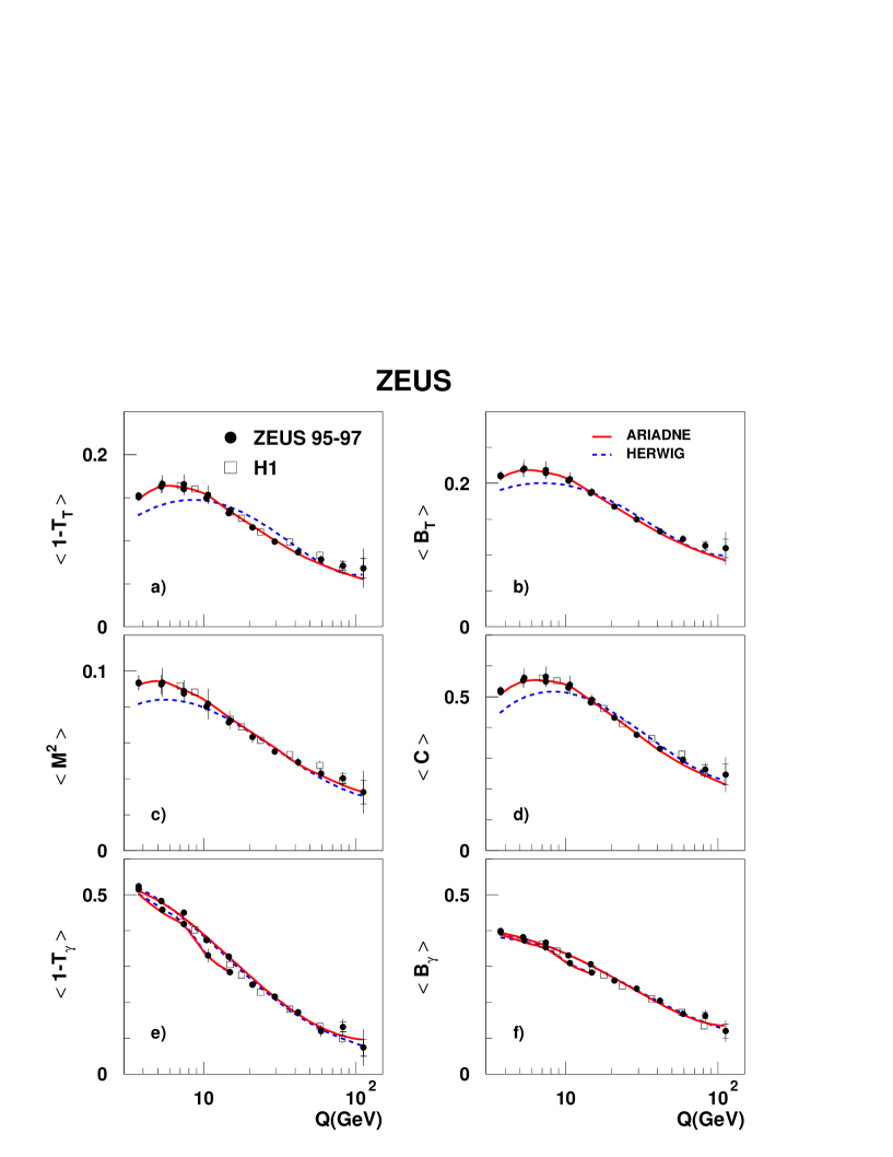
Figure 1: Comparison of the mean event-shape parameters (solid points) with ARIADNE and HERWIG predictions. The plots refer to a) thrust with respect to the thrust axis, b) jet broadening with respect to the thrust axis, c) invariant jet-mass squared, d) $C$-parameter, e) thrust with respect to the virtual photon axis, f) broadening with respect to the virtual photon axis. The data were corrected using ARIADNE. The inner error bars are statistical; the outer are statistical plus systematic added in quadrature. The open squares are H1 data, with statistical uncertainties which are in most cases covered by the symbol. In e) and f), where the $x$ variation is biggest, smoothed curves are drawn through the MC points for all $x$ $(Q^{2}>320{\,\text{Ge}\kern-0.39993pt\text{V\/}}^{2})$ and low $x$ $(Q^{2}<320{\,\text{Ge}\kern-0.39993pt\text{V\/}}^{2})$, and separately through the high-$x$ MC points $(Q^{2}<320{\,\text{Ge}\kern-0.39993pt\text{V\/}}^{2})$. A value of $\mathcal{E}_{lim}=0.1Q$ was used.

Figure 1 shows the corrected mean values of the event shapes as a function of $Q$, using $\mathcal{E}_{lim}=0.1Q$, together with the H1 measurements [7], with which there is good agreement. The mean values fall with $Q$ at the higher $Q$ values, and at lower $Q$ show an $x$ dependence at fixed $Q$ which is most pronounced for the variables measured with respect to the photon axis. Both here and with $\mathcal{E}_{lim}=0.25Q$ (not shown), good agreement is found with the predictions of ARIADNE over the entire $Q$ range. The agreement with HERWIG is less good, particularly for the variables $(1-T_{T})$, $B_{T}$, $M^{2}$ and $C$ at low $Q$. Although not used in the subsequent fits, the data for $Q^{2}<80{\,\text{Ge}\kern-0.39993pt\text{V\/}}^{2}$ are included for purposes of completeness, and to allow comparison with more extended theoretical fits if they become available.

The data were fitted to the sum of an NLO term, obtained from DISASTER++ or DISENT, plus a power correction as described above. The theoretical calculation neglects terms of the order of $1/{Q^{2}}$ [1]. Consequently, the analyses have been confined to the region $Q>9{\,\text{Ge}\kern-0.39993pt\text{V\/}}$, i.e. bins 7 - 16 in Table 1. With $\mu_{I}$ fixed at $2{\,\text{Ge}\kern-0.39993pt\text{V\/}}$, there are two parameters in Eq. (2), $\alpha_{s}(M_{Z})$ and $\overline{\alpha_{0}}$, that can be varied to obtain the best agreement between calculation and data.

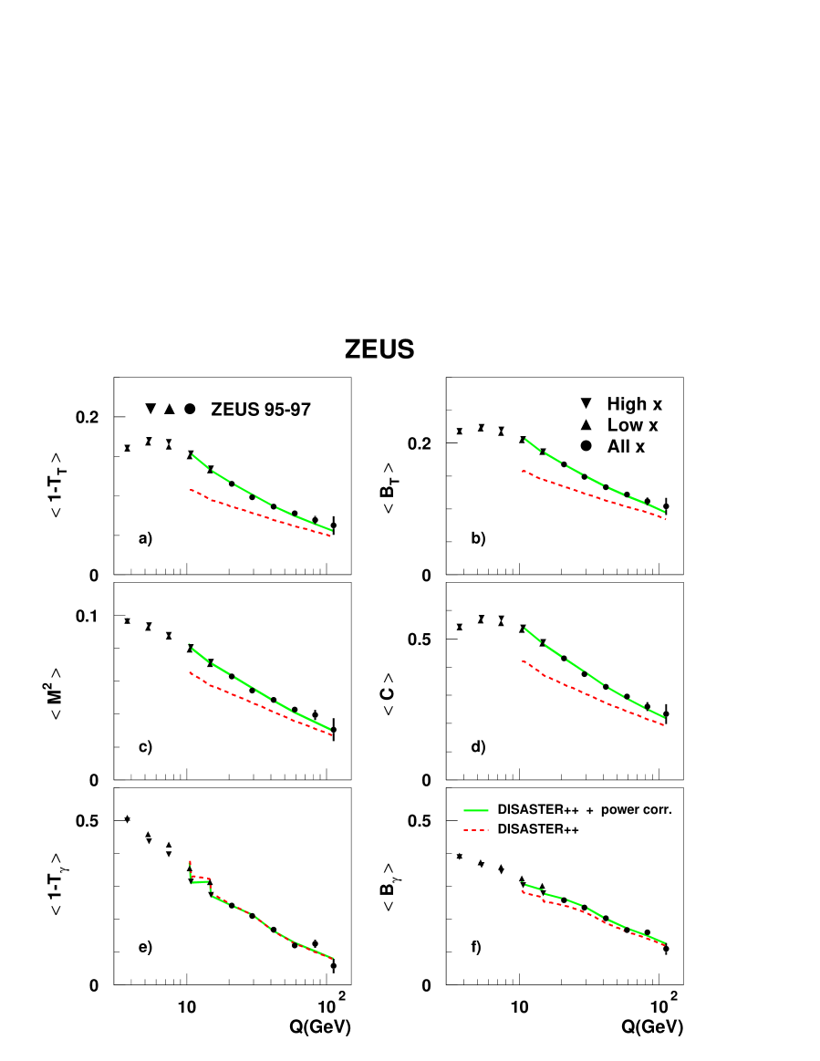
Figure 2: Fits to mean values of the shape variables versus $Q$, with $\mathcal{E}_{lim}=0.25Q$. Plots a) - f) are defined in the caption to Fig. 1. The lines join the fit values at the $Q$ values of the data: the solid line is the fitted NLO prediction from DISASTER++ plus the power correction, while the dashed line is the fitted DISASTER++ contribution alone. ‘High $x$’ and ‘low $x$’ refer to the subdivisions as defined in Table 1; ‘all $x$’ refers to the points with $Q>20{\,\text{Ge}\kern-0.39993pt\text{V\/}},$ which are not subdivided in $x$.

Two types of fit were studied: the offset method and the Hessian method. The offset method [41, 42] uses a $\chi^{2}$ defined using a diagonal error matrix with errors given by the statistical errors on the data points combined in quadrature with the uncorrelated errors arising from the limited statistics of the DISENT and DISASTER++ calculations. The Hessian method [43, 42] uses a full error matrix which includes correlated off-diagonal terms due to the systematic uncertainties. The fits obtained using the offset method are shown in Fig. 2. For the Hessian method, the four major systematics, namely those associated with $\delta$, the tightening and relaxation of the EFO angular and $p_{T}$ cuts, and the use of HERWIG, were included as off-diagonal terms in the error matrix. As expected, the $\chi^{2}$ is reduced with the Hessian method, and the fitted error, which includes the systematic contribution, is approximately a factor of two smaller than the systematic uncertainties estimated from the offset fits. For the variables $(1-T_{T})$, $B_{T}$, $M^{2}$ and $C$, the values of $\alpha_{s}$ from the two fit methods agree within the statistical uncertainties. For the $\alpha_{s}$ values from $(1-T_{\gamma})$ and $B_{\gamma}$, and for all evaluations of $\overline{\alpha_{0}}$, the two fit methods give results that in general differ by more than the statistical errors; they do however agree within the offset systematic uncertainty. The difference in the results of the fits originates primarily from the use of HERWIG in place of ARIADNE. The Hessian method relies upon Bayesian priors, specifically the assumption of Gaussian distributions, for the systematic uncertainties. There is no reason to believe that this assumption is correct for the dominating fragmentation systematic. Consequently, the results presented here are based on the offset method with its conservative estimate of systematic effects.

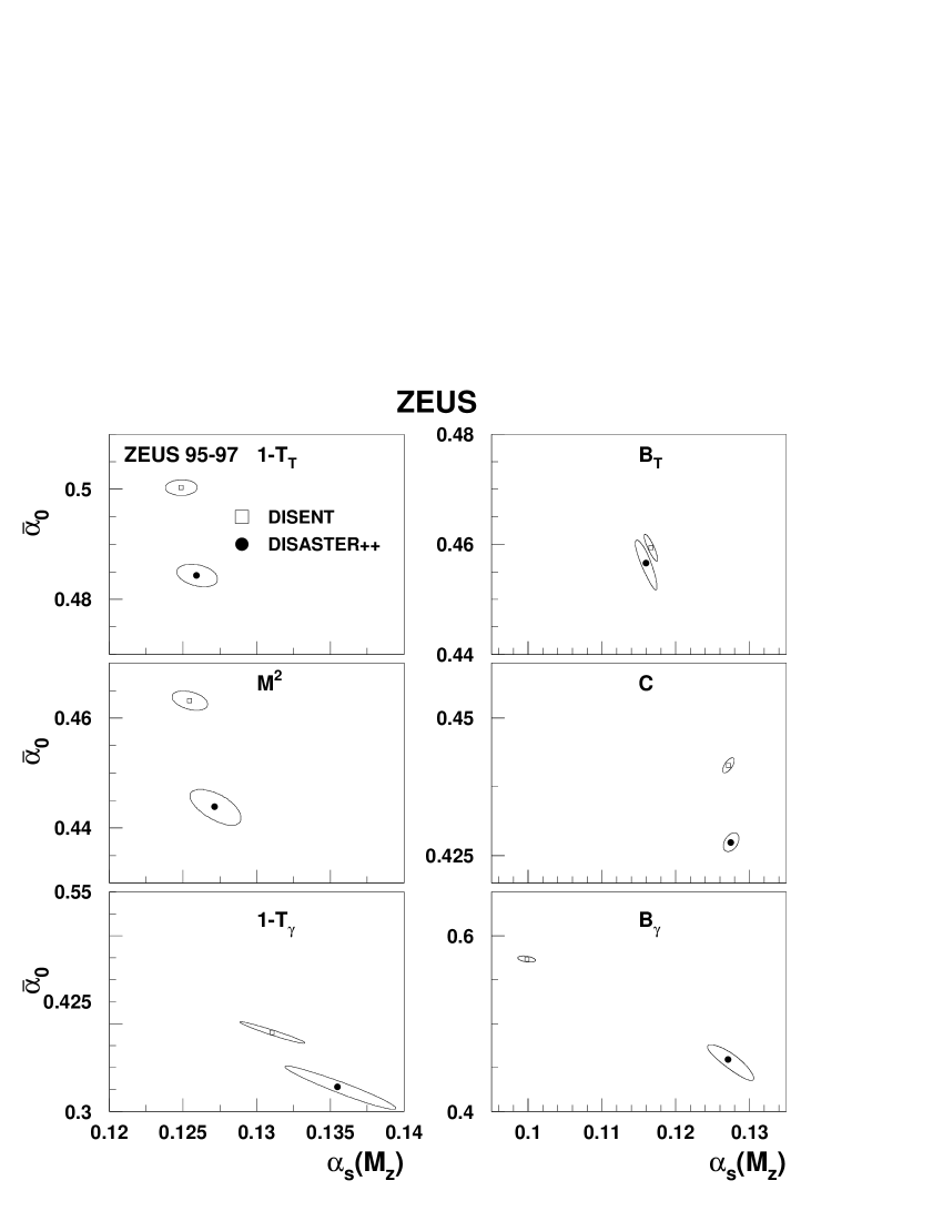
Figure 3: Contour plots for the parameters $\alpha_{s}(M_{Z})$ and $\overline{\alpha_{0}}$ fitted to the mean values of thrust and broadening measured with respect to the photon axis, jet-mass squared, $C$-parameter, and thrust and broadening measured with respect to the thrust axis. Results are shown for fits, using all data points for $Q^{2}>80{\,\text{Ge}\kern-0.39993pt\text{V\/}}^{2}$, based on DISASTER++ and DISENT with $\mathcal{E}_{lim}=0.25Q$. The contours show the one-standard-deviation limits determined using statistical uncertainties only.

The DISASTER++ calculation gives predictions in closer agreement with analytic calculations [40, 44] than does DISENT, which is believed to contain errors [45]. The fits using DISASTER++ for the NLO term are therefore taken to give the more reliable estimates of $\alpha_{s}$ and $\overline{\alpha_{0}}$. The DISENT-based analysis provides a check and facilitates comparison with H1, whose analysis used this program. Reasonable fits are obtained; those based on DISASTER++, using $\mathcal{E}_{lim}=0.25Q$, are shown in Fig. 2, while those for DISENT (not shown) are similar. The fitted power-correction term is substantial except for the variables that are based on the virtual-photon axis. The results of the fits using DISASTER++ and DISENT are compared in Fig. 3, where it can be seen that, with the exception of $B_{\gamma}$, $\alpha_{s}$ is the same within statistical errors for the two NLO calculations. For all variables, $\overline{\alpha_{0}}$ determined using DISASTER++ is smaller than when using DISENT.

As seen in Fig. 2, the data have a significant $x$-dependence at a given $Q$; consequently, fits have been made using the high-$x$ and low-$x$ selections, as well as to the full set of used bins. Results from the DISASTER++ fits are shown in the contour plots of Fig. 4.

To allow a direct comparison with the H1 results [7], Fig. 5 shows the determinations of $\alpha_{s}$ and $\overline{\alpha_{0}}$ using DISENT and $\mathcal{E}_{lim}=0.1Q$; as expected from the agreement of the measured data points (Fig. 1), the agreement in the fitted $\alpha_{s}$ and $\overline{\alpha_{0}}$ values is, in general, good. In particular, a low value of $\alpha_{s}$ for $B_{\gamma}$ is confirmed. The influence of the $\mathcal{E}_{lim}$ selection is also illustrated in Fig. 5, which shows, for DISENT, that the different selections lead to $\overline{\alpha_{0}}$ values that agree within about two standard deviations. In contrast, $\alpha_{s}$ appears more sensitive to $\mathcal{E}_{lim}$ for several of the variables. In general, it is found that $\mathcal{E}_{lim}=0.25Q$ gives a smaller variation of the fitted $\alpha_{s}$ and $\overline{\alpha_{0}}$ with $x$ than is found for $\mathcal{E}_{lim}=0.1Q$ (not shown). Given this, together with the theoretical preference for the higher $\mathcal{E}_{lim}$ [40], the central analysis is based on the data evaluated with $\mathcal{E}_{lim}=0.25Q$.

The experimental systematic uncertainties on $\alpha_{s}$ and $\overline{\alpha_{0}}$ were estimated by repeating the fits with the systematic variations described in Section 6. The largest effect resulted from correcting the data with HERWIG instead of ARIADNE. The use of HERWIG gave a systematic increase in $\alpha_{s}$ and a systematic decrease in $\overline{\alpha_{0}}$; these shifts are possibly attributable, respectively, to the use of parton showers rather than the colour-dipole model, and to the different fragmentation schemes used in the models. Also, HERWIG does not contain electroweak terms. The variables $(1-T_{\gamma})$ and $B_{\gamma}$ are in addition sensitive to the method of reconstructing the kinematic variables, owing to their dependence on the photon direction.

Figure  6 summarises the $\alpha_{s}$ and $\overline{\alpha_{0}}$ values from fits using the statistical errors, in order to indicate the degree of agreement between the different measurements. The systematic uncertainties on the data introduce highly correlated effects on the results obtained from the different shape variables, and so are not included here. The inconsistency which is evident between the different determinations is discussed below.

To estimate the theoretical uncertainties, the fragmentation and renormalisation scales were varied by a factor of two, and studies were made of the effects of changes to $\mu_{I}$ and to the Milan factor. To give an indication of the uncertainties due to mass effects, the data were reanalysed using the $E$-scheme [11]. It was found that $\alpha_{s}$ depends strongly on $\mu_{I}$, decreasing as $\mu_{I}$ is increased. If the model were robust, $\alpha_{s}$ should have little dependence on $\mu_{I}$.

The fit results including experimental and theoretical systematic uncertainties are collected in Tables 3 and 4. The dominant uncertainty comes from the variation of the renormalisation scale. The renormalisation-scale uncertainty quoted here follows the procedure employed in the $e^{+}e^{-}$ studies [4, 5, 6] using Eq. (3). If, following H1 [7], $Q$ in Eq. (3) were replaced by $\mu_{R}$, the theoretical uncertainty due to the $x_{\mu}$ variation would be approximately a factor of two larger. The influence of the $x$-dependent term in Eq. (5) was examined using the CTEQ5M proton structure [46]. While an improved fit to the data was obtained, the changes to the resulting $\alpha_{s}$ and $\overline{\alpha_{0}}$ values were less than their statistical uncertainties.

9 Discussion

From the results using DISASTER++, the following features are observed:

• $(1-T_{\gamma})$ requires a smaller hadronisation correction than $(1-T_{T})$ (Fig. 2), contrary to the theoretical expectation that the correction should be similar. This is responsible for the significantly different $\overline{\alpha_{0}}$ values for the two thrust variables;

• $(1-T_{\gamma})$ shows a larger $x$-dependence than $(1-T_{T})$; the $M^{2}$ and $C$ variables, whose definition does not depend on a choice of axis, show a small $x$ dependence (Fig. 2);

• a residual $x$ dependence in the fitted $\overline{\alpha_{0}}$ value obtained from ($1-T_{T}$), $(1-T_{\gamma})$ and $M^{2}$ but not from $B_{T}$, $B_{\gamma}$ and $C$ can be seen in Fig. 4. However, the $\overline{\alpha_{0}}$ values are also consistent with a similar small $x$ dependence in all four variables;

• the $\alpha_{s}$ values from all the variables except ($1-T_{\gamma}$) show no significant $x$ dependence.

There is an inconsistency between the $\overline{\alpha_{0}}$ values determined from $(1-T_{\gamma})$ and from the other variables. As noted earlier, there is an $x$ dependence in the data from $(1-T_{\gamma})$ that is not well described by the present model (Fig. 4). Consequently, the fitted values of $\alpha_{s}$ and $\overline{\alpha_{0}}$ for this variable are unlikely to be meaningful. The anomalous value of $\alpha_{s}$ may also be due to the fact that DISASTER++ does not take full account of initial-state gluon radiation or other effects related to the target remnant, which may affect the direction of the current-region system.

For the variables $(1-T_{T})$, $B_{\gamma}$, $M^{2}$ and $C$, the fitted $\alpha_{s}$ values are consistent within the statistical uncertainties. The variable $B_{T}$ gives an $\alpha_{s}$ value that differs from the other determinations, although its $\overline{\alpha_{0}}$ value agrees within $\pm 10\%$ with those from the other four variables. The inconsistency cannot be due to experimental or theoretical systematic uncertainties, including scale uncertainties, since these act in the same direction for all the variables. It may be taken to indicate that $B_{T}$ has a greater sensitivity to higher-order corrections than the other variables.

A comparison with other measurements is of interest. With the exception of $(1-T_{\gamma})$, the present results for $\alpha_{s}$ and $\overline{\alpha_{0}}$ are consistent with those from $e^{+}e^{-}$ data within the substantial theoretical uncertainties. Using $e^{+}e^{-}$ data from a variety of experiments, Movilla Fernández et al. found good agreement between the means of the event-shape variables as a function of $\sqrt{s}$; in contrast with the observations of this paper, they obtained $\alpha_{s}$ values that were consistent within statistical errors for all the variables studied [4, 5, 6]. The $\overline{\alpha_{0}}$ values were likewise mutually compatible, with the possible exception of that from $M^{2}$. An overall consistency was claimed which confirmed the validity of the model in the $e^{+}e^{-}$ context and thus enabled an overall experimental value for $\alpha_{s}$ to be given.

In summary, the power correction method applied in DIS gives consistent values for $\alpha_{s}$ for the event-shape variables $(1-T_{T})$, $B_{\gamma}$, $M^{2}$ and $C$. The $\overline{\alpha_{0}}$ values for these variables agree to within $\pm 10\%$, which is consistent with the precision claimed for the model. The variables $(1-T_{\gamma})$ and $B_{T}$ give, respectively, $\overline{\alpha_{0}}$ and $\alpha_{s}$ values that are inconsistent with the other determinations. It must be concluded, therefore, that the power-correction model does not consistently describe all the shape variables in DIS. Consequently, no average $\alpha_{s}$ or $\overline{\alpha_{0}}$ values are quoted.

10 Summary

A measurement has been made of the mean values of the event-shape variables thrust $(T)$, broadening $(B)$, normalised jet mass $(M^{2})$ and $C$-parameter, using the ZEUS detector at HERA. The variables $T$ and $B$ were determined relative to the virtual photon axis and the thrust axis. The events were analysed in the Breit frame for the kinematic range $6\times 10^{-4}<x<0.6$, $10<Q^{2}<20\,480{\,\text{Ge}\kern-0.39993pt\text{V\/}}^{2}$ and $0.04<y<0.95$. The data are successfully described by the ARIADNE Monte Carlo model.

The $Q$ dependences of the mean event shapes have been fitted to NLO calculations from perturbative QCD with the DISASTER++ and DISENT programs together with the Dokshitzer-Webber non-perturbative power corrections, with the aim of determining $\alpha_{s}(M_{Z})$ and $\overline{\alpha_{0}}(\mu_{I})$. Such a model should give values of $\alpha_{s}$ and $\overline{\alpha_{0}}$ that are independent of the shape variable. Neither DISASTER++ nor DISENT fulfils these requirements for all variables.

Using DISASTER++, consistent values of $\alpha_{s}$ are obtained for the shape variables $(1-T_{T})$, $B_{\gamma}$, $M^{2}$ and $C$, with $\overline{\alpha_{0}}$ values that agree to within $\pm 10\%$. The $\overline{\alpha_{0}}$ value from $(1-T_{\gamma})$ and the $\alpha_{s}$ value from $B_{T}$ are in disagreement with the other determinations. With the exception of $(1-T_{\gamma})$, the present values are consistent with those measured in $e^{+}e^{-}$ annihilation, to within the theoretical uncertainties. There is consistency with the results from H1.

The power correction method provides a successful description of the data for all event-shape variables studied. Nevertheless, the lack of consistency of the $\alpha_{s}$ and $\overline{\alpha_{0}}$ determinations obtained in deep inelastic scattering, together with the dependence of the results on Bjorken $x$, suggest the importance of higher-order processes that are not yet included in the model employed in this analysis. These effects must be understood before a reliable value of $\alpha_{s}$ can be quoted using the present method.

Bin	$Q^{2}\;({\,\text{Ge}\kern-0.39993pt\text{V\/}}^{2}$)	$x$	Bin	$Q^{2}\;({\,\text{Ge}\kern-0.39993pt\text{V\/}}^{2}$)	$x$
1	10 - 20	0.0006 - 0.0012	9	160 - 320	0.0024 - 0.010
2	10 - 20	0.0012 - 0.0024	10	160 - 320	0.01 - 0.05
3	20 - 40	0.0012 - 0.0024	11	320 - 640	0.01 - 0.05
4	20 - 40	0.0024 - 0.010	12	640 - 1280	0.01 - 0.05
5	40 - 80	0.0012 - 0.0024	13	1280 - 2560	0.025 - 0.150
6	40 - 80	0.0024 - 0.010	14	2560 - 5120	0.05 - 0.25
7	80 - 160	0.0024 - 0.010	15	5120 - 10240	0.06 - 0.40
8	80 - 160	0.01 - 0.050	16	10240 - 20480	0.10 - 0.60

Table 1: The kinematic boundaries of the bins in $x$ and $Q^{2}$. The power-correction fits use bins 7 - 16, apart from the fits denoted ‘high $x$’ and ‘low $x$’, which omit bins 7, 9 and bins 8, 10, respectively.

Bin	$1-T_{T}$	$B_{T}$	$M^{2}$	$C$	$1-T_{\gamma}$	$B_{\gamma}$
1	$0.1595\pm 0.0010\pm 0.0046$	$0.2172\pm 0.0009\pm 0.0060$	$0.0967\pm 0.0006\pm 0.0039$	$0.540\pm 0.003\pm 0.014$	$0.508\pm 0.002\pm 0.009$	$0.3932\pm 0.0010\pm 0.0066$
2	$0.1609\pm 0.0010\pm 0.0041$	$0.2185\pm 0.0009\pm 0.0059$	$0.0965\pm 0.0006\pm 0.0042$	$0.544\pm 0.003\pm 0.013$	$0.499\pm 0.002\pm 0.018$	$0.3892\pm 0.0010\pm 0.0108$
3	$0.1672\pm 0.0011\pm 0.0078$	$0.2223\pm 0.0010\pm 0.0094$	$0.0924\pm 0.0007\pm 0.0054$	$0.565\pm 0.003\pm 0.023$	$0.458\pm 0.003\pm 0.003$	$0.3731\pm 0.0011\pm 0.0013$
4	$0.1708\pm 0.0009\pm 0.0102$	$0.2248\pm 0.0008\pm 0.0123$	$0.0941\pm 0.0005\pm 0.0079$	$0.575\pm 0.002\pm 0.031$	$0.437\pm 0.002\pm 0.004$	$0.3644\pm 0.0009\pm 0.0044$
5	$0.1620\pm 0.0020\pm 0.0070$	$0.2155\pm 0.0014\pm 0.0056$	$0.0871\pm 0.0009\pm 0.0032$	$0.556\pm 0.004\pm 0.015$	$0.426\pm 0.004\pm 0.003$	$0.3580\pm 0.0020\pm 0.0020$
6	$0.1679\pm 0.0010\pm 0.0114$	$0.2204\pm 0.0009\pm 0.0122$	$0.0880\pm 0.0006\pm 0.0060$	$0.572\pm 0.003\pm 0.033$	$0.3968\pm 0.0024\pm 0.0015$	$0.3452\pm 0.0011\pm 0.0012$
7	$0.1500\pm 0.0004\pm 0.0050$	$0.2040\pm 0.0004\pm 0.0049$	$0.0791\pm 0.0002\pm 0.0030$	$0.5314\pm 0.0010\pm 0.0143$	$0.3547\pm 0.0010\pm 0.0031$	$0.3238\pm 0.0005\pm 0.0016$
8	$0.1536\pm 0.0005\pm 0.0110$	$0.2061\pm 0.0004\pm 0.0097$	$0.0808\pm 0.0003\pm 0.0084$	$0.5403\pm 0.0013\pm 0.0300$	$0.3149\pm 0.0012\pm 0.0190$	$0.3031\pm 0.0006\pm 0.0096$
9	$0.1322\pm 0.0007\pm 0.0013$	$0.1866\pm 0.0006\pm 0.0020$	$0.0703\pm 0.0004\pm 0.0008$	$0.483\pm 0.002\pm 0.006$	$0.3130\pm 0.0020\pm 0.0050$	$0.3009\pm 0.0009\pm 0.0029$
10	$0.1347\pm 0.0006\pm 0.0054$	$0.1875\pm 0.0005\pm 0.0053$	$0.0718\pm 0.0003\pm 0.0051$	$0.489\pm 0.002\pm 0.017$	$0.2742\pm 0.0013\pm 0.0071$	$0.2789\pm 0.0007\pm 0.0045$
11	$0.1150\pm 0.0008\pm 0.0027$	$0.1676\pm 0.0007\pm 0.0033$	$0.0628\pm 0.0004\pm 0.0032$	$0.431\pm 0.002\pm 0.010$	$0.242\pm 0.002\pm 0.005$	$0.2574\pm 0.0011\pm 0.0026$
12	$0.0982\pm 0.0012\pm 0.0017$	$0.1489\pm 0.0011\pm 0.0024$	$0.0543\pm 0.0007\pm 0.0017$	$0.375\pm 0.003\pm 0.006$	$0.210\pm 0.003\pm 0.004$	$0.235\pm 0.002\pm 0.002$
13	$0.086\pm 0.002\pm 0.002$	$0.133\pm 0.002\pm 0.002$	$0.0487\pm 0.0010\pm 0.0021$	$0.330\pm 0.005\pm 0.006$	$0.168\pm 0.004\pm 0.008$	$0.203\pm 0.003\pm 0.003$
14	$0.078\pm 0.003\pm 0.004$	$0.122\pm 0.003\pm 0.005$	$0.043\pm 0.002\pm 0.002$	$0.295\pm 0.009\pm 0.011$	$0.120\pm 0.007\pm 0.013$	$0.167\pm 0.005\pm 0.006$
15	$0.069\pm 0.005\pm 0.004$	$0.112\pm 0.006\pm 0.004$	$0.039\pm 0.003\pm 0.003$	$0.260\pm 0.015\pm 0.012$	$0.125\pm 0.012\pm 0.015$	$0.160\pm 0.009\pm 0.012$
16	$0.062\pm 0.012\pm 0.015$	$0.104\pm 0.013\pm 0.017$	$0.030\pm 0.007\pm 0.009$	$0.233\pm 0.035\pm 0.035$	$0.058\pm 0.022\pm 0.031$	$0.110\pm 0.018\pm 0.018$

Table 2: Mean event-shape variables in the bins defined in Table 1. The first uncertainty is statistical and the second is systematic.

Variable	$1-T_{T}$	$B_{T}$	$M^{2}$	$C$	$1-T_{\gamma}$	$B_{\gamma}$
$\boldsymbol{\alpha_{s}}\mathbf{(M_{Z})}$	$\mathbf{0.1258}$	$\mathbf{0.1159}$	$\mathbf{0.1271}$	$\mathbf{0.1274}$	$\mathbf{0.1354}$	$\mathbf{0.1270}$
stat. error	$\pm 0.0013$	$\pm 0.0013$	$\pm 0.0016$	$\pm 0.0010$	$\pm 0.0028$	$\pm 0.0026$
stat.$+$sys. unc.	$\pm 0.0040$	$\pm 0.0026$	$\pm 0.0040$	$\pm 0.0021$	$\pm 0.0132$	$\pm 0.0102$
$\chi^{2}/dof$	$2.8$	$1.3$	$2.1$	$1.5$	$2.5$	$1.8$
correlation	$-0.25$	$-0.80$	$-0.60$	$0.26$	$-0.93$	$-0.84$
$x_{F}=0.5$	$-0.0007$	$-0.0001$	$-0.0004$	$-0.0007$	$+0.0088$	$+0.0025$
$x_{F}=2.0$	$+0.0009$	$+0.0008$	$+0.0003$	$+0.0007$	$-0.0008$	$+0.0036$
$x_{\mu}=0.5$	$-0.0068$	$-0.0067$	$-0.0080$	$-0.0067$	$-0.0088$	$-0.0222$
$x_{\mu}=2.0$	$+0.0083$	$+0.0081$	$+0.0090$	$+0.0082$	$+0.0084$	$+0.0053$
${\cal{M}}=1.19$	$+0.0025$	$+0.0018$	$+0.0024$	$+0.0029$	$+0.0032$	$+0.0014$
${\cal{M}}=1.79$	$-0.0021$	$-0.0017$	$-0.0022$	$-0.0025$	$-0.0027$	$-0.0012$
$\mu_{I}=1\leavevmode\nobreak\ {\,\text{Ge}\kern-0.39993pt\text{V\/}}$	$+0.0054$	$+0.0042$	$+0.0053$	$+0.0063$	$+0.0069$	$+0.0029$
$\mu_{I}=4\leavevmode\nobreak\ {\,\text{Ge}\kern-0.39993pt\text{V\/}}$	$-0.0059$	$-0.0047$	$-0.0061$	$-0.0068$	$-0.0075$	$-0.0039$
E-scheme	$+0.0040$	$+0.0028$	$+0.0029$	$+0.0030$	$+0.0025$	$+0.0010$
$\mathbf{Total}$	$\mathbf{+0.0117}$	$\mathbf{+0.0101}$	$\mathbf{+0.0118}$	$\mathbf{+0.0114}$	$\mathbf{+0.0197}$	$\mathbf{+0.0128}$
$\mathbf{uncertainty}$	$\mathbf{-0.0101}$	$\mathbf{-0.0088}$	$\mathbf{-0.0111}$	$\mathbf{-0.0101}$	$\mathbf{-0.0178}$	$\mathbf{-0.0248}$

Table 3: Fitted results for $\alpha_{s}(M_{Z})$ using the NLO prediction from DISASTER++ and $\mathcal{E}_{lim}=0.25Q$. The quoted $\chi^{2}$ is that from the offset-method fit using statistical uncertainties and DISASTER++. The third line is the total experimental uncertainty from the statistical and experimental systematic uncertainties added in quadrature. The quoted $\chi^{2}$ is from the offset-method fit using statistical uncertainties and DISASTER++. The fifth row gives the correlation coefficients between the fitted values of $\alpha_{s}(M_{Z})$ and $\overline{\alpha_{0}}$ (see next Table). The $x_{F}$, $x_{\mu}$, $\cal{M}$, and $\mu_{I}$ rows give the theoretical systematic uncertainties due to variations on the fragmentation and renormalisation scales, the Milan factor and the lower limit for the perturbative calculation, respectively; the $x_{F}$ and $x_{\mu}$ values denote factors by which the respective scale values are varied. The systematic effect of using the $E$-scheme rather than the $P$-scheme is given in the final row of systematic uncertainties. The total uncertainty is the total experimental uncertainty added in quadrature with the theoretical uncertainties.

Variable	$1-T_{T}$	$B_{T}$	$M^{2}$	$C$	$1-T_{\gamma}$	$B_{\gamma}$
$\boldsymbol{\overline{\alpha_{0}}}\;\mathbf{(2\leavevmode\nobreak\ GeV)}$	$\mathbf{0.4843}$	$\mathbf{0.4566}$	$\mathbf{0.4440}$	$\mathbf{0.4274}$	$\mathbf{0.3286}$	$\mathbf{0.4593}$
stat. error	$\pm 0.0020$	$\pm 0.0041$	$\pm 0.0030$	$\pm 0.0017$	$\pm 0.0187$	$\pm 0.0171$
stat.$+$sys. error	$\pm 0.0264$	$\pm 0.0139$	$\pm 0.0439$	$\pm 0.0144$	$\pm 0.0993$	$\pm 0.0815$
$x_{F}=0.5$	$+0.0030$	$+0.0019$	$+0.0006$	$+0.0018$	$-0.1173$	$-0.0491$
$x_{F}=2.0$	$-0.0017$	$-0.0034$	$+0.0002$	$-0.0006$	$+0.0421$	$-0.0128$
$x_{\mu}=0.5$	$+0.007$	$+0.056$	$+0.016$	$+0.007$	$+0.009$	$+0.256$
$x_{\mu}=2.0$	$-0.002$	$-0.033$	$-0.007$	$-0.003$	$+0.029$	$-0.135$
${\cal{M}}=1.19$	$+0.0363$	$+0.0390$	$+0.0223$	$+0.0235$	$-0.0402$	$+0.0250$
${\cal{M}}=1.79$	$-0.0282$	$-0.0296$	$-0.0192$	$-0.0200$	$+0.0187$	$-0.0197$
E-scheme	$+0.0163$	$+0.0101$	$+0.0134$	$+0.0127$	$+0.0052$	$+0.0103$
$\mathbf{Total}$	$\mathbf{+0.0483}$	$\mathbf{+0.0706}$	$\mathbf{+0.0535}$	$\mathbf{+0.0312}$	$\mathbf{+0.1137}$	$\mathbf{+0.2700}$
$\mathbf{uncertainty}$	$\mathbf{-0.0387}$	$\mathbf{-0.0467}$	$\mathbf{-0.0484}$	$\mathbf{-0.0248}$	$\mathbf{-0.1589}$	$\mathbf{-0.1664}$

Table 4: Fitted results for $\overline{\alpha_{0}}$  defined at $\mu_{I}=2$ GeV, using the NLO prediction from DISASTER++ and $\mathcal{E}_{lim}=0.25Q$. Other definitions are given in the caption to Table 3.

Figure 4: Contour plots for $\alpha_{s}(M_{Z})$ and $\overline{\alpha_{0}}$ fitted to the mean values of the event-shape variables. The fits are based on DISASTER++, with $\mathcal{E}_{lim}=0.25Q$. The contours show the one-standard-deviation limits determined using statistical uncertainties only. The high-$x$ and low-$x$ selections are as defined in Table 1, while ‘all data’ uses all measured bins for $Q^{2}>80{\,\text{Ge}\kern-0.39993pt\text{V\/}}^{2}$.

Figure 5: Contour plots for $\alpha_{s}(M_{Z})$ and $\overline{\alpha_{0}}$ fitted to the mean values of the event-shape variables. The fits are based on DISENT, using all data for $Q^{2}>80{\,\text{Ge}\kern-0.39993pt\text{V\/}}^{2}$, with energy cuts $\mathcal{E}_{lim}=0.1Q$ (open squares) and $0.25Q$ (filled circles). The contours show the one-standard-deviation limits determined using statistical uncertainties only. The rectangles enclose the associated pairs of points to guide the eye.

Figure 6: Contour plots for $\alpha_{s}(M_{Z})$ and $\overline{\alpha_{0}}$ fitted to the mean values of the event-shape variables. The fits are based on DISASTER++, with $\mathcal{E}_{lim}=0.25Q$. The contours show the one-standard-deviation limits determined using statistical uncertainties only. For further comments, see text; the full systematic errors, which are strongly correlated between the different variables, are given in Tables 3 and 4.

References

-
[1]
Yu. L. Dokshitzer and B. R. Webber, Phys. Lett. B 352, 451 (1995);
Yu. L. Dokshitzer and B. R. Webber, Phys. Lett. B 404, 321 (1997);
Yu. L. Dokshitzer et al., Nucl. Phys. B 511, 396 (1998); Erratum: ibid. B 593, 729 (2001). - [2] Yu. L. Dokshitzer, G. Marchesini and G. P. Salam, Eur. Phys. J. (direct)C 3, 1 (1999).
- [3] M. Dasgupta and B. R. Webber, Eur. Phys. J. C 1, 539 (1998).
-
[4]
DELPHI Collaboration, P. Abreu et al., Z. Phys. C 73, 229 (1997);
DELPHI Collaboration, P. Abreu et al., Phys. Lett. B 456, 322 (1999). -
[5]
P. A. Movilla Fernández
et al. and the JADE Collaboration, Eur. Phys. J. C 1, 461 (1998);
O. Biebel et al. and the JADE Collaboration, Phys. Lett. B 459, 326 (1999). - [6] P. A. Movilla Fernández et al., Eur. Phys. J. C 22, 1 (2001).
-
[7]
H1 Collaboration, C. Adloff et al., Phys. Lett. B 406, 256 (1997);
H1 Collaboration, C. Adloff et al., Eur. Phys. J. C 14, 255 (2000), [Addendum – Eur. Phys. J. C 18, 417 (2000)]. - [8] R. P. Feynman, Photon-Hadron Interactions, Benjamin, NY (1972).
- [9] D. Graudenz, DISASTER++ Program Manual, Version 1.0.1 (1997), hep-ph/9710244.
-
[10]
S. Catani and M. H. Seymour, Nucl. Phys. B 485, 291 (1997)
[Erratum – Nucl. Phys. B 510, 503 (1997)];
M. H. Seymour, DISENT Program Manual, Version 0.1, (1997). - [11] G. P. Salam and D. Wicke, JHEP 0105, 61 (2001).
- [12] ZEUS Collaboration, M. Derrick et al., Phys. Lett. B 297, 205 (1992).
-
[13]
M. Derrick et al., Nucl. Instr. Meth. A 309, 77 (1991);
A. Andresen et al., Nucl. Instr. Meth. A 309, 101 (1991);
A. Caldwell et al., Nucl. Instr. Meth. A 321, 356 (1992);
A. Bernstein et al., Nucl. Instr. Meth. A 338, 23 (1993). -
[14]
N. Harnew et al., Nucl. Instr. Meth. A 279, 290 (1989);
B. Foster et al., Nucl. Phys. (Proc. Supp.) B 32, 181 (1993);
B. Foster et al., Nucl. Instr. Meth. A 338, 254 (1994). - [15] S. Bentvelson et al., Proc. Workshop on Physics at HERA, Vol. I, W. Buchmüller and G. Ingelman (eds.), DESY (1992) p. 23; K. C. Hoeger, ibid., p. 43.
-
[16]
H. Abramowicz, A. Caldwell and R. Sinkus,
DESY 95-094 (1995);
R. Sinkus and T. Voss, Nucl. Instr. Meth. A 389, 160 (1997). - [17] ZEUS Collaboration, S. Chekanov et al., Eur. Phys. J. C 21, 443 (2001).
- [18] ZEUS Collaboration, J. Breitweg et al., Eur. Phys. J. C 6, 43 (1999).
- [19] R. Brun et al., GEANT3, CERN DD/EE/84-1 (1987).
- [20] K. Charchuła, G. Schuler and H. Spiesberger, Comp. Phys. Comm. 81, 381 (1994).
- [21] G. Ingelman, A. Edin and J. Rathsman, Comp. Phys. Comm. 101, 108 (1997).
- [22] A. Kwiatkowski, H. Spiesberger and H.-J. Möhring, Proc. Workshop on Physics at HERA, Vol. I, W. Buchmüller and G. Ingelman (eds.), DESY (1992) p. 1294.
- [23] L. Lönnblad, Comp. Phys. Comm. 71, 15 (1992).
- [24] L. Lönnblad, Proc. Workshop Monte Carlo Generators for HERA Physics, DESY-PROC-1999-02, A. T. Doyle et al. (eds.), (1999) p. 47.
- [25] B. Andersson et al., Phys. Rep. 97, 31 (1983).
- [26] T. Sjöstrand, Comp. Phys. Comm. 82, 74 (1994).
- [27] G. Marchesini et al., Comp. Phys. Comm. 67, 465 (1992).
- [28] G. Marchesini and B. R. Webber, Nucl. Phys. B 310, 461 (1988).
- [29] G. J. McCance, Ph. D. Thesis, University of Glasgow (2001), unpublished.
-
[30]
H. Jung, RAPGAP program manual
http://www.quark.lu.se/hannes/rapgap.html - [31] CTEQ Collaboration, H. L. Lai et al., Phys. Rev. D55, 1280 (1997).
- [32] ZEUS Collaboration, M. Derrick et al., Z. Phys. C 67, 93 (1995).
- [33] ZEUS Collaboration, M. Derrick et al., Z. Phys. C 59, 231 (1993).
- [34] ZEUS Collaboration, J. Breitweg et al., Eur. Phys. J. C 11, 251 (1999).
- [35] ZEUS Collaboration, J. Breitweg et al., Eur. Phys. J. C 11, 427 (1999).
- [36] W. T. Giele, E. W. N. Glover and J. Yu, Phys. Rev. D 53, 120 (1996).
-
[37]
Yu. L. Dokshitzer et al., JHEP 9805, 3 (1998);
M. Dasgupta and B. R. Webber, JHEP 9810, 1 (1999). - [38] Yu. L. Dokshitzer, G. Marchesini and G. P. Salam, Eur. Phys. J. C 3, 1 (1999).
- [39] M. Dasgupta and G. P. Salam, Eur. Phys. J. C 24, 213 (2002).
- [40] V. Antonelli, M. Dasgupta and G. P. Salam, JHEP 0002, 1 (2000).
-
[41]
S. I. Alekhin, hep-ex/0005042;
M. Botje, J. Phys. G 28, 779 (2002). - [42] ZEUS Collaboration, S. Chekanov et al., DESY 02-105 (2002), to be published in Phys. Rev. D.
-
[43]
D. Stump et al., Phys. Rev. D 65, 014012 (2001);
J. Pumplin et al., Phys. Rev. D 65, 014013 (2001). - [44] G. J. McCance, Proc. Workshop Monte Carlo Generators for HERA Physics, DESY-PROC-1999-02, A. T. Doyle et al., (eds.) (1999) p. 151; hep-ph/9912481.
- [45] M. Dasgupta and G. P. Salam, JHEP 0208, 32 (2002).
-
[46]
CTEQ Collaboration, H. L. Lai et al., Eur. Phys. J. C 12, 375 (2000);
H. Plothow-Besch, Users Manual - Version 8.04, W5051 PDFLIB 2000.04.17 CERN ETT/TT;
H. Plothow-Besch, Int. J. Mod. Phys. A 10, 2901 (1995).