Inclusive $\eta^{\prime}$ Production From The $\Upsilon(1S)$

Abstract

Using the CLEO II detector at CESR, we measure the $\eta^{\prime}$ energy spectra in $\Upsilon(1S)$ decays, that we compare with models of the $\eta^{\prime}g^{*}g$ form-factor. This form-factor especially at large $\eta^{\prime}$ energies may provide an explanation of the large rate for $B\to X_{s}\eta^{\prime}$. Our data do not support a large anomalous coupling at higher $q^{2}$ and thus the large $\eta^{\prime}$ rate remains a mystery, possibly requiring a non-Standard Model explanation.

I Introduction

There are several interesting, unexplained phenomena in $B$ decays. First of all, the total production of charm and charmonium seems about 10% low charm_deficit , especially when coupled with a $B$ semileptonic branching ratio of (10.4$\pm$0.3)% PDG . Secondly, CLEO observed a very large rate of $\eta^{\prime}$ in the momentum range from 2 to 2.7 GeV/c with a branching fraction of $(6.2\pm 1.6\pm 1.3^{+0.0}_{-1.5})\times 10^{-4}$ Browder . The BABAR experiment has confirmed this large rate Babaretap . The production of $\eta^{\prime}$ mesons is believed to occur dominantly via the $b\to sg$ mechanism, as strongly suggested by observation of the two-body decay $B\to\eta^{\prime}K$. One explanation of the large $\eta^{\prime}$ rate is that the $b\to sg$ rate is not 1% as expected in the Standard Model, but is enhanced by new physics to be at the 10% level. This would also explain the charm deficit problem.

An alternative explanation is that of an anomalously strong coupling between the $\eta^{\prime}$ and two gluons Atwood:1997bn ; Hou:1997wy ; Kagan:1997sg . The process $b\to sg$ followed by the two gluon coupling to the $\eta^{\prime}$ is shown in Fig. 1.

Figure 1: Diagram for $b\to sg\eta^{\prime}$.

Experimentally, the hadronic mass associated with $X_{s}$ sometimes is a $K$, $\sim$10%, and even more rarely a $K^{*}$, $\sim$1%; in fact, most of the rate has the mass of the $X_{s}$ system larger than 1.8 GeV.

Since the $\eta^{\prime}$ is mostly the flavor singlet $\eta_{1}$, as the $\eta-\eta^{\prime}$ mixing angle is between $10^{\circ}-20^{\circ}$, the effective $\eta^{\prime}g^{*}g$ coupling can be written as Kagan02

$$H(q^{2})\varepsilon_{\alpha\beta\mu\nu}q^{\alpha}k^{\beta}\varepsilon^{\mu}_{1}\varepsilon^{\nu}_{2},$$ (1)

where $q=p_{b}-p_{s}$ is the four-momentum of the virtual hard gluon $(g^{*})$, $k$ is the four-momentum of the soft “on-shell” gluon $(g)$, and $H(q^{2})$ is the $g^{*}g\eta^{\prime}$ transition form factor.

Chen and Kagan Kagan02 have shown that the region of the $q^{2}$ relevant in the process $b\to sg\eta^{\prime}$ can also be accessed in high energy $\eta^{\prime}$ production in $\Upsilon(1S)$ decay. Thus constraints can be put on the $H(q^{2})$ from the $\eta^{\prime}$ spectrum in $\Upsilon(1S)\to ggg$ decays. $H(0)$ is found from the rate of $J/\psi\to\gamma\eta^{\prime}$ decays as $\sim$1.8 GeV^-1.

Three choices for the form factor shape $H(q^{2})$ are shown in Fig. 2: (a) a slowly falling form factor from Hou and Tseng Hou:1997wy , $H(q^{2})=2.1~{}{\rm GeV}^{-1}\alpha_{s}(q^{2})/\alpha_{s}(m^{2}_{\eta^{\prime}})$; (b) a rapidly falling form factor representative of perturbative QCD calculations, $H(q^{2})=1.7$ GeV^-1m${}^{2}_{\eta^{\prime}}/(q^{2}-m^{2}_{\eta^{\prime}})$ at $q^{2}>$ 1 GeV²; (c) an intermediate example with $H(q^{2})\propto 1/(q^{2}+2.2^{2}{\rm GeV}^{2})$ Kagan02 . In (b) and (c) the form factor at $q^{2}\approx m_{\eta{\prime}}^{2}$ has been matched onto the value given in (a), which is fixed by the QCD anomaly Hou:1997wy . The parametrization of the form factor in (b) follows from a simple model in which the $\eta^{\prime}$ is coupled perturbatively to two gluons through quark loops Kagan:1997sg . With the choice $H(0)=1.7$ GeV^-1 it compares well with the perturbative QCD form factors obtained by other authors Ali:2000ci ; Muta .

Figure 2: Three choices for the form factor $H(q^{2})$ plotted against $\sqrt{q^{2}}$: (a) the slowly falling form factor, (b) a rapidly falling form factor representative of perturbative QCD calculations, (c) an intermediate example (adapted from Kagan02 ).

We will compare the theoretical predictions for $H(q^{2})$ with data taken on the $\Upsilon(1S)$ resonance with the CLEO II detector at the CESR storage ring. Some information on this topic has been extracted by Kagan from ARGUS data Kagan_argus .

II Data Sample and Analysis Method

In this study we use 80 pb^-1 of CLEO II data recorded at the $\Upsilon(1S)$ resonance (9.46 GeV), containing $1.862\times 10^{6}$ $\Upsilon(1S)$ events. We also use off-resonance continuum data collected below the $\Upsilon(4S)$ resonance (10.52 GeV) with a total integrated luminosity of 1193 pb^-1.

The theoretical predictions referred to in this paper are made for $\Upsilon(1S)$ decays into three gluons ($ggg$). In order to compare our measurement to them we have to correct for the $\Upsilon(1S)\to\gamma^{*}\to q\bar{q}$ contribution, whose size is given by

$${\cal{B}}(\Upsilon(1S)\to\gamma^{*}\to q\bar{q})=R\cdot{\cal{B}}(\Upsilon(1S)\to\mu^{+}\mu^{-})=(8.8\pm 0.3)\%,$$ (2)

where $R_{\sqrt{s}\approx 9.5}=3.56\pm 0.07$ Ammar:1997sk and the ${\cal{B}}(\Upsilon(1S)\to\mu^{+}\mu^{-})$ is taken as $(2.48\pm 0.06)\%$ PDG .

Although several processes can contribute to inclusive $\eta^{\prime}$ production in $\Upsilon(1S)$ decays, it is believed that the soft processes including fragmentation populate only the low $q^{2}$ or equivalently the low Z region, where

$${\rm Z}\equiv E_{\eta^{\prime}}/E_{beam}=2E_{\eta^{\prime}}/M(\Upsilon(1S)).$$ (3)

Thus in the large Z region significant $\eta^{\prime}$ production would indicate a large $\eta^{\prime}g^{*}g$ coupling.

The CLEO II detector, described in detail elsewhere CLEO_II had a high resolution electromagnetic calorimeter comprised of 7800 CsI crystals surrounding a precision tracking system.

We detect $\eta^{\prime}$ mesons using the decay channel: $\eta^{\prime}\to\eta\pi^{+}\pi^{-}$ with a branching fraction of $44\%$, and $\eta\to\gamma\gamma$ with a branching fraction of $39\%$. We identify single photons based on their shower shape and the non-proximity of charged tracks. Those photon pairs within the “good barrel” region of the detector, $|\cos\theta|<0.707$ (where $\theta$ is the angle with respect to the beam), that have invariant masses consistent with the $\eta$ mass within 3 standard deviations are constrained to have the invariant mass of the $\eta$. For $\eta$ mesons coming from low energy $\eta^{\prime}$ candidates ($\rm Z<0.5$) the background from $\pi^{\circ}$ decay is large, and thus the candidate photons are also required not to be from a possible $\pi^{\circ}$ decay. We then add two opposite sign pions and form the $\eta\pi^{+}\pi^{-}$ invariant mass.

The $\eta\pi^{+}\pi^{-}$ invariant mass spectra are shown in Fig. 3 for $\Upsilon(1S)$ and for off-resonance continuum data. The spectra are fit with a Gaussian function for signal and second order polynomial function for background. The numbers of reconstructed $\eta^{\prime}$ are extracted from the fit. We find $\rm 1486\pm 137\ \eta^{\prime}$ from the $\Upsilon(1S)$ data, and $\rm 4062\pm 174\ \eta^{\prime}$ from the off-resonance data.

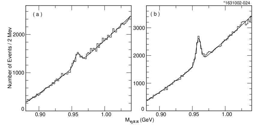
Figure 3: The $\eta\pi^{+}\pi^{-}$ invariant mass spectrum reconstructed from $\Upsilon(1S)$ data (left), and off resonance data at 10.52 GeV (right) fit with Gaussian functions for signal and second order polynomials for background.

To measure the energy spectrum we reconstruct $\eta^{\prime}$ candidates in Z intervals. We choose the Z steps as 0.1. The invariant mass spectra are fit with the same functional form as used for Fig. 3. Here we fix the mass of the $\eta^{\prime}$ to our average value over all Z; the Monte Carlo simulation shows that the mass measurement should be independent of $\eta^{\prime}$ energy. We extract the width of the signal Gaussian distribution from Monte Carlo simulation for each Z bin and perform a smooth fit as a function of Z. The smoothed values are used in the fit as fixed parameters. The $\eta\pi^{+}\pi^{-}$ Z dependent mass spectra are shown in Fig. 4 and Fig. 5 for $\Upsilon(1S)$ and off-resonance data, respectively.

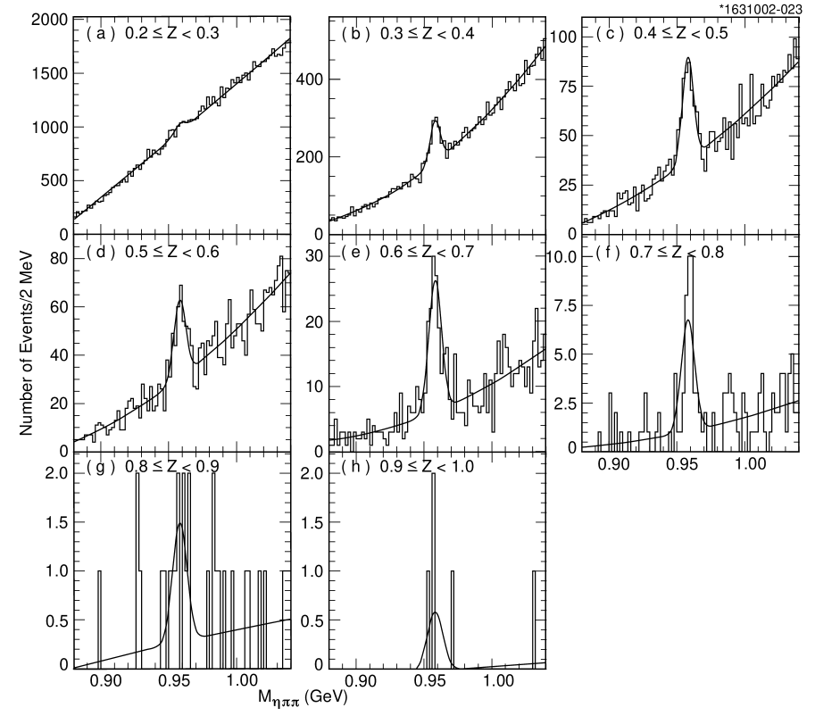
Figure 4: The $\eta\pi^{+}\pi^{-}$ invariant mass spectra in different Z ranges reconstructed from $\Upsilon(1S)$ data, fit with a Gaussian function for signal and a second order polynomial for background.

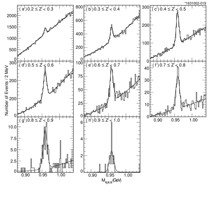
Figure 5: The $\eta\pi^{+}\pi^{-}$ invariant mass spectra in different Z ranges reconstructed from off-resonance data, fit with a Gaussian function for signal and a second order polynomial for background.

In order to extract decay rates we need to correct our raw event yields by efficiencies. These may not be equal for different intermediate states, i.e. $q\bar{q}$ versus $ggg$. The hadronic events at $\Upsilon(1S)$ energy arise from different sources: about 4 nb is $q\bar{q}$ from continuum $\rm e^{+}e^{-}$ collisions, about 2 nb from $\Upsilon(1S)\to\gamma^{*}\to q\bar{q}$, 18 nb from $ggg$, and 0.5 nb from $\gamma gg$ from the $\Upsilon(1S)$. The first two have same event topology and reconstruction efficiencies. We use the $q\bar{q}$ Monte Carlo generator to simulate these events. The $\gamma gg$ events are similar to that of $ggg$ and have a relatively small cross-section; thus we treat them the same way as $ggg$ events. We use the $ggg$ Monte Carlo generator to simulate this part.

We rely on off-resonance continuum data to estimate the $q\bar{q}$ contribution in $\Upsilon(1S)$ data. However, the continuum data were taken for continuum subtraction in $\Upsilon(4S)$ studies. The center of mass (CM) energy (10.52 GeV) is close to $\Upsilon(4S)$ mass (10.58 GeV), but more than 1 GeV higher than $\Upsilon(1S)$ mass (9.46 GeV). The difference of reconstruction efficiency due to this energy difference is not negligible. We thus use different $q\bar{q}$ simulations for continuum data and $\Upsilon(1S)$ data.

The energy difference also affects the Z spectrum of $\eta^{\prime}$ from continuum Monte Carlo as shown in Fig. 6-(a). The solid line is the $\rm E_{\eta^{\prime}}/E_{beam}$ distribution for the $\Upsilon(1S)$ data (9.46 GeV) and dashed line for the continuum data (10.52 GeV). The low limits are 0.202 and 0.182 respectively. The discrepancy is significant, especially at low energy. In order to use our continuum data at 10.52 GeV we need to map it to 9.46 GeV. To do so we rely on the continuum Monte Carlo. We take the two Monte Carlo $\eta^{\prime}$ shape distributions at 10.52 and 9.46 GeV, denoted by ${\cal P}_{10.52}(z)$ and ${\cal P}_{9.46}(z)$ and numerically integrate them to satisfy the relation:

$$\int^{{\rm Z}^{\prime}_{10.52}}_{0}{\cal P}_{10.52}(z)dz=\int^{{\rm Z}^{\prime}_{9.46}}_{0}{\cal P}_{9.46}(z)dz~{}~{},$$ (4)

where Z${}^{\prime}_{10.52}$ is fixed and a value for Z${}^{\prime}_{9.46}$ is determined. The data points on Fig. 6-(b) show the difference in Z${}^{\prime}_{9.46}-$Z${}^{\prime}_{10.52}$ as a function of Z${}^{\prime}_{10.52}$ (or equivalently $\rm Z_{0}$ in following function). We fit the points with a fourth order polynomial function to define the mapping analytically as

$$\rm Z=-0.215\times 10^{-2}+1.2238\ Z_{0}-0.6879\ Z_{0}^{2}+0.8277\ Z_{0}^{3}-0.3606\ Z_{0}^{4}\ .$$ (5)

The simplest mapping would be a linear conversion $Z=0.025+0.975\times Z_{0}$, shown as dotted line in Fig. 6-(b). We use this alternative to estimate the systematic uncertainty due to the mapping.

That this mapping works is demonstrated in Fig. 6-(a), where the spectra shown as open circles is the mapped spectrum according to Equation 5. It overlaps well with the Monte Carlo spectrum generated at 9.46 GeV.

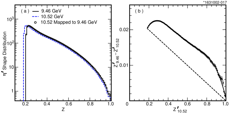
Figure 6: a) The Z $=E_{\eta^{\prime}}/E_{beam}$ distributions from Monte Carlo simulation. The solid line is the Z=$E_{\eta^{\prime}}/E_{beam}$ spectrum for an energy of 9.46 GeV, the dashed line is the spectrum for 10.52 GeV and the open circles are the mapped spectrum from 10.52 GeV. b) The data points show the difference in the Z values at 9.46 and 10.52 GeV as a function of the Z value at 10.52 GeV. The solid curve is a fit to a fourth order polynomial. The dotted line shows the mapping of the linear conversion.

The $\eta^{\prime}$ production rate is smaller at 9.46 GeV because of less available energy. From the $q\bar{q}$ generator we found that the production rate is 93.6% that of 10.52 GeV. This factor is also considered in estimation of the $\eta^{\prime}$ production from $q\bar{q}$ events.

The mapping for continuum data is derived from the model-dependent Monte Carlo spectrum. If the real data and the Monte Carlo are very different then the systematic uncertainty due to this mapping could be large. To check this, we compared the measured $\rm E_{\eta^{\prime}}/E_{beam}$ spectrum with the generated spectrum. Fortunately, the spectra agree reasonably well and the systematic uncertainty due to this source is negligible.

We now turn to estimating the detection efficiencies. Shown in Fig. 7 are the efficiencies estimated with different models and different energies for a) without the $\pi^{\circ}$ veto, and b) with the $\pi^{\circ}$ veto. In the real data we applied $\pi^{\circ}$ veto to $\eta^{\prime}$ candidates with Z $<$ 0.5. Comparing with the efficiency from 9.46 GeV $q\bar{q}$ events, the efficiency from $ggg$ events is roughly 15% higher, and the efficiency from 10.52 GeV $q\bar{q}$ events is roughly 7% lower. The main source of such difference is the event shape. The $ggg$ events are more spherical while the higher energy $q\bar{q}$ events are more jetty.

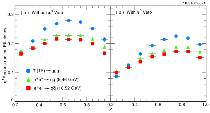
Figure 7: The $\eta^{\prime}$ reconstruction efficiencies as function of Z for different MC samples a) without a $\pi^{o}$ veto, and b) with a $\pi^{o}$ veto in the photon selection.

III Extraction of the $\eta^{\prime}$ Spectrum from $\Upsilon(1S)$ Decays

The $\Upsilon(1S)$ data sample can be broken down into three parts as described in the previous section:

$$N_{all}=N_{\Upsilon(1S)\to ggg}+N_{\Upsilon(1S)\to q\bar{q}}+N_{e^{+}e^{-}\to q\bar{q}}\ .$$

The first one has different reconstruction efficiencies from the other two. For the contribution from continuum $(e^{+}e^{-}\to q\bar{q}$) events, we multiply the number from off-resonance events at 10.52 GeV, mapped using Equation 5, by a factor $f_{e^{+}e^{-}\to q\bar{q}}$ defined as:

$$N(\eta^{\prime})_{e^{+}e^{-}\to q\bar{q}}(9.46\ {\rm GeV})=N(\eta^{\prime})_{e^{+}e^{-}\to q\bar{q}}(10.52\ {\rm GeV})\times f_{e^{+}e^{-}\to q\bar{q}},$$ (6)

where

$$f_{e^{+}e^{-}\to q\bar{q}} = \frac{80.4}{1193}\times\frac{1/9.46^{2}}{1/10.52^{2}}\times 0.9356\times\frac{\epsilon_{9.46}}{\epsilon_{10.52}}$$ (7)

$$= 0.078\times\frac{\epsilon_{9.46}}{\epsilon_{10.52}}\ ,$$

where the first factor is the relative luminosities, the second the energy squared dependence of the cross section, the third the relative $\eta^{\prime}$ yield and $\epsilon$ is the $Z$-dependent reconstruction efficiency for $q\bar{q}$ events as shown Fig. 7.

We also want to evaluate the yield from $\Upsilon(1S)\to\gamma^{*}\to q\overline{q}$. Since we know that $\sigma_{\Upsilon(1S)\to\mu^{+}\mu^{-}}=0.555\pm 0.022\ {\rm nb}$ and $\sigma_{e^{+}e^{-}\to\mu^{+}\mu^{-}}(9.46\ {\rm GeV})=1.12\ {\rm nb}$ Chen:1989ms , we derive the factor to be used in the $N_{\Upsilon(1S)\to q\bar{q}}$ estimation as:

$$f_{\Upsilon(1S)\to q\bar{q}} = f_{e^{+}e^{-}\to q\bar{q}}\times\frac{R\cdot\sigma_{\Upsilon(1S)\to\mu^{+}\mu^{-}}}{R\cdot\sigma_{e^{+}e^{-}\to\mu^{+}\mu^{-}}}$$ (8)

$$= 0.0387\times\frac{\epsilon_{9.46}}{\epsilon_{10.52}}.$$

In Table 1 we list the number of reconstructed $\eta^{\prime}$ over all $Z$ and in the high $Z$ region for various $\Upsilon(1S)$ and continuum yields (only statistical errors are shown). Note that the total numbers of signal from $\Upsilon(1S)$ data and off-resonance data in this table are the sum of all $Z$ bins derived bin per bin, as we need to use $Z$-dependent efficiencies.

Sample	All Z	$\rm Z>0.7$
$\Upsilon(1S)$ data	1494 $\pm$ 120	46.0 $\pm$ 8.1
off-resonance	4294 $\pm$ 130	257.1 $\pm$ 17.3
$\Upsilon(1S)\to ggg$	972 $\pm$ 120	13.9 $\pm$ 8.1
$\Upsilon(1S)\to q\bar{q}$	173 $\pm$ 5	10.6 $\pm$ 0.7
Continuum $q\bar{q}$	349 $\pm$ 11	21.5 $\pm$ 1.4
$\Upsilon(1S)\to ggg,q\bar{q}$	1145 $\pm$ 120	24.5 $\pm$ 8.1

Table 1: Number of reconstructed $\eta^{\prime}$ from $\Upsilon(1S)$ and off-resonance data and the breakdown categories of $\Upsilon(1S)$ data. Also listed are for samples with $\rm Z>0.7$.

The measured $\Upsilon(1S)\to\eta^{\prime}X$ branching fractions are listed in Table 2 both for Z $>$ 0.7 and for all Z. In the large Z region for 3 gluon decays, we do not have a statistically significant signal and thus derive a 90% confidence level upper limit of ${\cal B}(\Upsilon(1S)\to ggg\to\eta^{\prime}X)_{Z>0.7}/{\cal B}(\Upsilon(1S)\to ggg)<3.4\times 10^{-4}$. We describe the systematic errors below.

Mode	All Z	Z $>$ 0.7
${\cal B}(\Upsilon(1S)\to\eta^{\prime}X)$	$(2.8\pm 0.4\pm 0.2)$ %	$(3.1\pm 0.9\pm 0.3)\times 10^{-4}$
${\cal B}(\Upsilon(1S)\to ggg\to\eta^{\prime}X)/{\cal B}(\Upsilon(1S)\to ggg)$	$(2.8\pm 0.5\pm 0.2)$%	$(1.9\pm 1.1\pm 0.2)\times 10^{-4}$
${\cal B}(\Upsilon(1S)\to q\bar{q}\to\eta^{\prime}X)/{\cal B}(\Upsilon(1S)\to q\bar{q})$	$(4.2\pm 0.2\pm 0.4)$ %	$(16.8\pm 1.1\pm 1.7)\times 10^{-4}$

Table 2: Branching fractions of $\Upsilon(1S)$ to $\eta^{\prime}$ mesons, for all decays, three gluon decays and quark-antiquark decays for the entire $\eta^{\prime}$ energy spectrum and for Z $>$ 0.7. The errors after the values give the statistical and systematic uncertainties, respectively.

The sources of systematic uncertainties are listed in Table 3 along with estimates of their sizes. The total systematic errors on branching ratios are $\pm 10\%$ for $q\bar{q}$ sample (independent of Z), $\pm 11\%$ for $ggg$ sample at $Z>0.7$, and $\pm 8.6\%$ for the rest.

Sources	$ggg$ ($Z>0.7$)	$q\bar{q}$	All others
Reconstruction efficiency of $\pi^{\pm}$	4.4	4.4	4.4
Reconstruction efficiency of $\eta$	5	5	5
Number of $\eta^{\prime}$ from fit	2	2	2
Total number of $\Upsilon(1S)$	2.4	2.4	2.4
${\cal B}(\eta^{\prime}\to\pi^{+}\pi^{-}\eta)$	3.4	3.4	3.4
${\cal B}(\Upsilon(1S)\to q\bar{q})^{\dagger}$	-	3.2	-
Ratio of integrated luminosity lumerr	2.9	1	-
$\sigma_{\Upsilon(1S)\to\mu^{+}\mu^{-}}$	3.6	4	-
Z mapping	6	3	3
Total	11	10	8.6
$\dagger$ We use ${\cal B}(\Upsilon(1S)\to(q\bar{q}))=(8.83\pm 0.28)\%$.

Table 3: The systematic uncertainties (in %) from different sources on the branching fraction measurements for the 3 gluon sample for Z $>$ 0.7, the $q\bar{q}$ sample, and both the 3 gluon sample for all Z and the total $\Upsilon(1S)$ sample.

We also measure the differential branching fractions as a function of Z as shown in Fig. 8. In these plots only the statistical error is shown, which dominates the total error.

We define three relevant differential branching ratio’s $dn/dZ$ as:

$$\frac{dn(ggg)}{dZ} = \frac{d{\cal B}(\Upsilon(1S)\to ggg\to\eta^{\prime}X)}{dZ\times{\cal B}(\Upsilon(1S)\to ggg)}~{}~{},$$

$$\frac{dn(q\bar{q})}{dZ} = \frac{d{\cal B}(\Upsilon(1S)\to q\bar{q}\to\eta^{\prime}X)}{dZ\times{\cal B}(\Upsilon(1S)\to q\bar{q})}~{}~{},$$

$$\frac{dn(1S)}{dZ} = \frac{d{\cal B}(\Upsilon(1S)\to\eta^{\prime}X)}{dZ}~{}~{}.$$ (9)

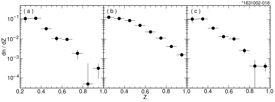
Figure 8: The differential branching fraction $dn/dZ$ as defined in context for a) $\Upsilon(1S)\to ggg\to\eta^{\prime}X$, b) $\Upsilon(1S)\to q\bar{q}\to\eta^{\prime}X$, and c) $\Upsilon(1S)\to\eta^{\prime}X$.

Listed in Table 4 are the differential branching fractions in Z intervals for $\Upsilon(1S)$ decays to $\eta^{\prime}$ for $ggg$ and $q\bar{q}$ subsamples and all decays.

Z	$\Upsilon(1S)\to(ggg)$	$\Upsilon(1S)\to(q\bar{q})$	All $\Upsilon(1S)$
0.2 - 0.3	11164 $\pm$ 4471	13205 $\pm$ 1253	10503 $\pm$ 3740
0.3 - 0.4	11624 $\pm$ 1314	11250 $\pm$ 685	10716 $\pm$ 1099
0.4 - 0.5	3381 $\pm$ 558	8898 $\pm$ 416	3614 $\pm$ 467
0.5 - 0.6	1067 $\pm$ 300	5030 $\pm$ 272	1336 $\pm$ 251
0.6 - 0.7	963 $\pm$ 181	2321 $\pm$ 166	1011 $\pm$ 151
0.7 - 0.8	184 $\pm$ 92	1116 $\pm$ 102	252 $\pm$ 77
0.8 - 0.9	5 $\pm$ 50	415 $\pm$ 59	41 $\pm$ 42
0.9 - 1.0	31 $\pm$ 22	153 $\pm$ 36	40 $\pm$ 19
0.7 - 1.0	19 $\pm$ 11	168 $\pm$ 11	31 $\pm$ 9
sum of all	2842 $\pm$ 471	4239 $\pm$ 153	2751 $\pm$ 394

Table 4: Differential branching fractions of $\eta^{\prime}$ ($\times 10^{-5}$). The last two rows are total branching fractions. The branching fractions in columns 2 and 3 are normalized to the total branching fraction of $\Upsilon(1S)\to(ggg)$ and $\Upsilon(1S)\to(q\bar{q})$ respectively, while the last column is normalized to all $\Upsilon(1S)$ decay. The errors are statistical only, the systematic errors on the absolute normalization for column 1 is 8.6% for Z $<$ 0.7, 11% for Z $>$ 0.7, and 10% and 8.6% for columns 2 and 3, respectively.

In the Z spectrum of $\eta^{\prime}$ mesons produced via $ggg$, there is an excess above an apparent exponential decrease for 0.6 $<$ Z $<$ 0.7, corresponding to a recoil mass opposite the $\eta^{\prime}$ in the range 5.3 to 6.1 GeV excess . However, a detailed study did not reveal any narrow structures. A possible explanation is that there is more than one process contributing to this distribution. We note also that the $q\bar{q}$ has much larger rates at high Z than $ggg$.

IV Comparison with Theory and Conclusions

Fig. 9 shows the Z spectrum of the $\eta^{\prime}$ measured in this paper compared with the spectra predicted by the three different models described above. The models are expected to dominate $\eta^{\prime}$ production only for Z$>0.7$, with other fragmentation based processes being important at lower Z. The measurement strongly favors a rapidly falling $q^{2}$ dependence of the ${g^{*}g\eta^{\prime}}$ form factor predicted by pQCD Ali:2000ci ; Muta , and ruling out other models.

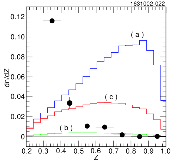
Figure 9: The measured $dn/dZ$ spectrum of $\Upsilon(1S)\to(ggg)\to\eta^{\prime}X$ compared with theoretical predictions. Shown in dots are the measurement in this study. Shown in lines are different theoretical predictions: a) a slowly falling form factor, b) a rapidly falling form factor, and c) intermediate form factor Kagan02 . These predictions are valid only in the region Z $>$ 0.7.

In conclusion, we have made the first measurement of the $\eta^{\prime}$ energy spectrum from $\Upsilon(1S)\to ggg$ decays. Our data are not consistent with an enhanced $\eta^{\prime}g^{*}g$ coupling at large $\eta^{\prime}$ energies. Thus, the large observed $\eta^{\prime}$ yield near end point of the charmless $B$ decay spectrum cannot be explained by a large $\eta^{\prime}g^{*}g$ form-factor. Therefore, new physics has not been ruled out and may indeed be present in rare $b$ decays.

V Acknowledgments

We thank Alex Kagan for providing us with his calculations and we thank A. Kagan and A. Ali for useful discussions on the theoretical models. We gratefully acknowledge the effort of the CESR staff in providing us with excellent luminosity and running conditions. M. Selen thanks the Research Corporation, and A.H. Mahmood thanks the Texas Advanced Research Program. This work was supported by the National Science Foundation and the U.S. Department of Energy.

References

(1) A. L. Kagan, Phys. Rev. D51, 6196 (1995); M. Neubert,
“Heavy Flavour Physics,” CERN-TH/95-307 [hep-ph/9511409] (1995).
(2)
K. Hagiwara et al., Phys. Rev. D66, 010001 (2002).
(3)
T. E. Browder et al. [CLEO Collaboration], Phys. Rev. Let. 81, 1786 (1998), [hep-ex/9804018]
(4)
They measure in the momentum range between
2.0 and 2.7 GeV/c. See
B. Aubertet al. [BABAR Collaboration], “Study of Semi-inclusive
Production of Mesons in Decays,” SLAC-PUB-8979 [hep-ex/0109034]
(2001),
(5)
D. Atwood and A. Soni,
Phys. Lett. B 405, 150 (1997) [hep-ph/9704357].
(6)
W. S. Hou and B. Tseng,
Phys. Rev. Lett. 80, 434 (1998) [hep-ph/9705304].
(7)
A. L. Kagan and A. A. Petrov, [hep-ph/9707354]; A. Kagan,
in proceedings of the Seventh International Symposium on Heavy Flavor
Physics, Santa Barbara CA, July 1997, [hep-ph/9806266].
(8) A. L. Kagan, “Beyond the Standard Model in B Decays:
Three Topics,” in proceedings of 9th Int. Symp. On Heavy Flavor Physics,
CalTech, Pasadena, Ca., Sept. 2001, ed. Ryd and Porter, AIP, Melville, NY,
p310, [hep-ph/0201313]; Y. Chen and A. L. Kagan, Univ. of Cincinnati preprint in
preparation.
(9)
A. Ali and A. Y. Parkhomenko,
Phys. Rev. D 65, 074020 (2002)[hep-ph/0012212].
(10)
T. Muta and M.-Z. Yang, Phys. Rev. D 61, 054007 (2000) [hep-ph/9909484].
(11)
The ARGUS collaboration had an integrated luminosity of 32
pb-1 on the resonance. A. Kagan
Kagan02 cites the upper limit in the higher Z region
, where he extracted the number
from an unpublished thesis A. Zimmermann, Diplom Thesis,
University of Dortmund, April 1992 where no continuum subtraction
was attempted. (See also, H. Albrecht et al. ARGUS collaboration,
Z. Phys. C 58, 1199-206 (1993)).
(12)
R. Ammar et al. [CLEO Collaboration],
Phys. Rev. D 57, 1350 (1998) [hep-ex/9707018].
(13)
Y. Kubota et al. (CLEO), Nucl. Instr. And Meth. A320, 66 (1992).
(14)
W. Y. Chen et al. [CLEO Collaboration],
Phys. Rev. D39, 3528 (1989).
(15)
We use the ratio of integrated luminosities of and
off-resonance data in calculating and
. The uncertainty of this ratio is
about . The uncertainty of , 4%, also affects . These latter two directly affect the branching
fraction in the sample with uncertainties of 1% and
4% respectively. The effects of these two sources to the overall
and the sample branching fractions are negligible except for
the branching fraction measurement of high energy in the
samples, where there are and
uncertainties.
(16)
We fit the Z distribution in the range 0.3 Z 1, not
including the point 0.6 Z 0.7, to an assumed inherent
exponential shape and determined that this point is 3.3 standard
deviations in excess.