A Multi-variate Discrimination Technique Based on Range-Searching

Abstract

We present a fast and transparent multi-variate event classification technique, called PDE-RS, which is based on sampling the signal and background densities in a multi-dimensional phase space using range-searching. The employed algorithm is presented in detail and its behaviour is studied with simple toy examples representing basic patterns of problems often encountered in High Energy Physics data analyses. In addition an example relevant for the search for instanton-induced processes in deep-inelastic scattering at HERA is discussed. For all studied examples, the new presented method performs as good as artificial Neural Networks and has furthermore the advantage to need less computation time. This allows to carefully select the best combination of observables which optimally separate the signal and background and for which the simulations describe the data best. Moreover, the systematic and statistical uncertainties can be easily evaluated. The method is therefore a powerful tool to find a small number of signal events in the large data samples expected at future particle colliders.

1 Introduction

In High Energy Physics one is frequently confronted with the task of finding a small number of distinctive (signal) events among a large number of background events. This problem is often tackled by simply applying cuts, motivated by models describing these characteristic events, on measured characteristic observables. However, in particular in complex cases where many observables have to be used, more powerful techniques exist, which are based on probability density estimation (PDE) or which employ Neural Networks (NNs). They first combine the observables to a single one, called “discriminant” on which then a cut to separate signal from background is applied. These methods were widely used in the search for the top-quark at the TEVATRON [1, 2, 3] and will play a major role in the search for the Higgs boson in the future [4]. For a general introduction to multi-variate discrimination techniques see [5].

A drawback of these methods is often that they come as a “black box” which provides few insights on the statistical and systematic uncertainties of the results obtained with the method. We will present here a novel discrimination technique based on counting signal and background events in small multi-dimensional boxes. The simple event counting allows to transparently handle the involved uncertainties and to separate signal and background events with a power similar to NNs. The event counting is done using a fast range-searching algorithm. Its speed allows to use very large data samples required in analyses where a high reduction of background is necessary or to scan a large number of observables for those which give the best separation of signal and background and for which the Monte Carlo simulations describe the data best. This technique has already been used in recent searches at HERA [6, 7].

2 Probability Density Estimation Techniques

In order to classify an event it is necessary to estimate the probability $p(\mathbf{x})$ that an event is of the signal class, given $d$ measured properties (called observables in the following) $\mathbf{x}=(x_{1},\ldots,x_{d})$. An estimate $\tilde{p}(\mathbf{x})$ of $p(\mathbf{x})$ can be obtained by employing Monte Carlo simulators which approximate the probability densities of the signal $\tilde{\rho}_{s}(\mathbf{x})\approx\rho_{s}(\mathbf{x})$ and of the background events $\tilde{\rho}_{b}(\mathbf{x})\approx\rho_{b}(\mathbf{x})$ by sampling the $d$-dimensional phase space with simulated events. The probability that a particular event belongs to the signal class is then given by

$$\tilde{p}(\mathbf{x})=\frac{\tilde{\rho}_{s}(\mathbf{x})}{\tilde{\rho}_{s}(\mathbf{x})+\tilde{\rho}_{b}(\mathbf{x})}\approx p(\mathbf{x})=\frac{\rho_{s}(\mathbf{x})}{\rho_{s}(\mathbf{x})+\rho_{b}(\mathbf{x})}.$$ (1)

The function $\tilde{p}(\mathbf{x})$ is a so called “Discriminant”, since it assigns to any given combination of measured observables a single value which discriminates background from signal events.

Finding good approximations of the signal and background densities can be a rather difficult problem, especially in high dimensional cases. Here, histograming methods cannot be used because the number of required bins increases as $m^{d}$, if $m$ is the number of bins per dimension. This causes a dramatic increase in memory usage and a decrease of the available number of events per bin. The problem is aggravated by correlations among the observables which is often the case in High Energy Physics applications. Due to correlations, the phase space is commonly populated only in a sub-space of lower dimensionality, i.e. the intrinsic dimensionality of the problem actually is smaller. To overcome the problem of the high dimensionality, sometimes methods are employed, which try to deduce the multi-dimensional probability density from projections. These methods suffer from correlations among the observables, which are not modelled by the projections.

Kernel based PDE methods [2] sum up appropriately chosen kernel functions to model the probability density around the point $\mathbf{x}$:

$$\tilde{p}(\mathbf{x})=\frac{1}{Nh^{d}}\sum_{i=1}^{N}K\left(\frac{\mathbf{x}-\mathbf{x}_{i}}{h}\right),$$ (2)

where the sum runs over all sample events $\mathbf{x}_{i}$, $N$ is the total number of events in the data sample and $h$ is a smoothing parameter. For the kernel function $K$ often a Gaussian distribution is chosen:

$$K(\mathbf{x})=\frac{1}{(2\pi)^{d/2}}\exp\left(-\frac{1}{2}||\mathbf{x}||^{2}\right),$$ (3)

making the resulting distribution continuous and differentiable. Since for every event which is classified, eq. (2) needs to be evaluated involving the sum over all $N$ sample events, these methods are very time consuming for large data samples. To avoid this problem functions only defined in a small region around $x$ have to be used.

A powerful method to estimate $p(\mathbf{x})$ are artificial Neural Networks [5]. Their design is inspired by biological neurons. In a training phase they parameterise the probability density by linear combinations of smooth functions. Using training events of known type the free parameters, usually called weights, are adjusted. The convergence of this procedure is usually fast reducing the time requirements compared to kernel based PDE methods. Given sufficiently large NNs with a high number of nodes, even very complicated probability densities can be approximated. Their good performance and their fast applicability make them a good candidate to compare the new method with. In many problems a fast computing time is crucial to perform a meaningful reduction of input observables by studying combinations of them and is important to handle large data samples required in searches where the background needs to be strongly reduced.

3 Probability Density Estimation based on Range-Searching

3.1 The PDE-RS Method

The multi-variate probability density estimation technique based on range-searching (PDE-RS) counts the number of Monte Carlo generated signal and background events in the vicinity of an event which is to be classified. From the counted events the probability of this event to be of the signal class is derived. This is done in an efficient way using range-searching with an algorithm described below. Given the number of signal events $n_{s}$ and the number of background events $n_{b}$ in a small volume $V(\mathbf{x})$ around the point $\mathbf{x}$, we define a discriminant

$$D(\mathbf{x}):=\frac{n_{s}}{n_{s}+c\,n_{b}},$$ (4)

which for sufficiently small volumes $V(\mathbf{x})$ and a sufficiently high number of sample events gives a very good approximation of $p(\mathbf{x})$, if the normalisation constant $c$ is chosen such that the total number of simulated signal events is equal to $c$ times the total number of background events. $D(\mathbf{x})$ provides a good estimate of the local event density and prevents a wrong classification due to bad interpolation into regions where the Monte Carlo simulations provide no information. This happens, if methods try to fit the event density globally, as is done e.g. by Neural Networks. However, in the PDE-RS method a large number of Monte Carlo generated events is needed to densely populate the whole phase space. This can be a limiting factor, if the number of observables and thus the dimensionality of the problem is high. For the counting method, in the vicinity of each event to be classified a large number of events have to be counted — a potentially time-consuming task. This problem is known as “range-searching” in computer sciences.

Range-searching has been studied intensively since several years, because the problem to find a specific event in a large data sample occurs in all sorts of classification tasks. Powerful algorithms have been devised to tackle it [8, 9]. Two different classes of algorithms are usually applied: One which subdivides the entire volume of the observable space into small boxes and stores the events within the boxes in a linked list. Searching for an event then just involves looking up which boxes are in the vicinity of the event that is to be classified and then simply scan the linked list for events within a certain distance. The second class of algorithms use multi-dimensional binary trees to store the events. An algorithm of this class as described in [10] is used here. The advantage is that in contrast to the subdivision algorithm the extent of the observable space needs not to be known, that is the minima and maxima of the observables need not be calculated before. In addition, subdivision algorithms have a huge memory consumption if the dimensionality of the problem is large, since they have to store the pointers to the linked lists in an array of the dimension of the problem, even if no event lies in a box. Such a behaviour is, however, expected for High Energy Physics events, for which the observables describing their properties are in many cases correlated leaving a large fraction of the phase space empty.

3.2 The PDE-RS Algorithm

Figure 1: a) Signal events distributed in a $2$-dimensional phase space spanned by the observables $x_{1}$ and $x_{2}$. The numbers refer to the occurrence of the events in the data sample, b) the resulting binary tree to store the events and c) signal and background events in the $x_{1}$-$x_{2}$ plane. The open triangle depicts the event to be classified. The box around the triangle shows the region where events are considered to calculate the discriminant. The lines and numbers illustrate the way how the events in the box are found with the help of the binary tree. A detailed description can be found in the text.

The algorithm used for the event classification is based on the range-searching algorithm described in [10]. It allows to search through $N$ Monte Carlo generated events that sample the signal and background density within a time $\sim\log_{2}(N)$. To achieve this scaling of the algorithm with the total number of events, all $N$ events are first stored in two $d$-dimensional binary trees — one for the background and one for the signal events — as is sketched in figure 1 for a two-dimensional example: Consider a random sequence of signal events $e_{i}(x_{1},x_{2})$, $i=1\ldots 7$ shown in figure 1a with their position in $x_{1}-x_{2}$-space, which are to be stored in a binary tree. The first event in the sequence becomes by definition the topmost node of the tree. The second event $e_{2}(x_{1},x_{2})$ has a larger $x_{1}$-coordinate than the first event, therefore a new node is created for it and the node is attached to the first node as the right child (if the $x_{1}$-coordinate had been smaller, the node would have become the left child). Event $e_{3}$ has a larger $x_{1}$-coordinate than event $e_{1}$, it therefore should be attached to the right branch below $e_{1}$. Since $e_{2}$ is already placed at that position, now the $x_{2}$-coordinates of $e_{2}$ and $e_{3}$ are compared, and, since $e_{3}$ has a larger $x_{2}$, $e_{3}$ becomes the right child of the node with event $e_{2}$. Thus the tree is sequentially filled by taking every event and, while descending the tree, comparing its $x_{1}$ and $x_{2}$ coordinates with the events already in place. Whether $x_{1}$ or $x_{2}$ are used to compare depends on the level within the tree. On the first level, $x_{1}$ is used, on the second level $x_{2}$, on the third again $x_{1}$ and so on. The result for events $e_{i}$ is shown in figure 1b. The amount of time needed to fill the tree is $\sim\sum_{i=1}^{N}\log_{2}(i)=\log_{2}(N!)=\mathcal{O}(N\log_{2}(N))$. The last equality can be easily verified with the help of Sterling’s formula.

Finding all events within the tree which lie in a given box is done in a similar way by comparing the bounds of the box with the coordinates of the events in the tree. For example, if the whole box lies to the right of event $e_{1}$ as shown in figure 1c, then only events on the branch below and including $e_{2}$ need to be searched. This halves the number of events in question. Only if an event in a node lies within the bounds of the coordinates of the box that it is compared to, both its siblings need to be searched. Searching the tree once requires therefore an effort only $\sim\log_{2}(N)$. It needs to be noticed that the whole tree of Monte Carlo generated events needs to be kept in the main memory of the computer to have a reasonably fast access time when comparing the coordinates. Therefore, only the advent of computers with random access memory of the order of hundreds of megabyte made it possible to use millions of events to sample the signal and background densities.

Since the number of signal and background events used in the calculation of the probability density estimation is known at each point in the phase space, the uncertainty of this estimate due to the limited number of signal and background events can be calculated. By inspecting eq. (4) we find that the statistical error $\Delta D(\mathbf{x})$ is given by

$$\Delta D(\mathbf{x})=\sqrt{\left(\frac{c\,n_{b}}{\left(n_{s}+c\,n_{b}\right)^{2}}\Delta n_{s}\right)^{2}+\left(\frac{c\,n_{s}}{\left(n_{s}+c\,n_{b}\right)^{2}}\Delta n_{b}\right)^{2}},$$ (5)

where $\Delta n_{s}$ and $\Delta n_{b}$ are the statistical uncertainties of the signal and background respectively.

Usually the calculated discriminant values of samples of events are histogramed and the performance of the discrimination technique is estimated by applying cuts on this discriminant. For discriminant values falling into the same bin, the uncertainties are of course correlated, because they are derived from the same samples of signal and background events. Using the individual uncertainties on $D$ for each event according to eq. (5) would overestimate the systematic uncertainty. Instead, a good estimate of the systematic uncertainty of each histogram bin is given by using the total number of signal and background in eq. (5), which fall into the phase space region corresponding to the bin. We have used Monte Carlo experiments using statistically independent event samples to confirm the validity of this estimate.

In order to influence the uncertainty of the probability density estimate, the size of the box can be adapted. The lengths of the box edges are the only free parameters of the algorithm. In the following examples where the observables are produced in similar ranges (i.e. they have similar “scales”), the number of parameters is reduced by using a hyper cube with edges of equal size $2l$. In this case $l$ is the largest distance in the maximum norm of every counted event to the centre of the box. In practical applications, where the observables can have very different scales, the relative length of the edges can be deduced from histograms of the observables before the method is applied. The box size should be chosen large enough in order to have a reasonably small uncertainty on $D(\mathbf{x})$. For too large boxes, however, the precise mapping of the probability density onto boxes is not possible and therefore the achievable separation is reduced. As will be shown in the following, the performance of the PDE-RS method is not very sensitive with respect to the box size.

4 Properties of PDE-RS and Comparison to Neural Networks

In the following we will study the properties and the performance of the PDE-RS method using three simple examples chosen as prototypes of basic situations encountered in High Energy Physics data analyses. The performance, the needed computing time and the ease of applicability are compared to NNs. The following examples have been chosen:

1. Two Gaussian probability densities to study the simple case of uncorrelated observables, where most of the multi-variate discrimination techniques give good results.

2. Two strongly correlated observables, where an elementary variable transformation largely simplifies the classification problem, as example of a problem which can be easily solved, if the relations between the observables are known e.g. by insights into the acting physical laws. Such problems can easily be solved by a physicist when a small number of observables are involved, but can pose problems to classification algorithms.

3. A high dimensional example, where a physicist has difficulties to find a good separation by looking at the observable distributions and where the multi-variate discrimination techniques generally show their strength.

4.1 Bivariate Uncorrelated Gaussian Probability Densities

Figure 2: a) The phase space densities of background (open circles) and signal (full circles) of two simple bivariate Gaussian distributions with displaced means and equal widths b) the probability density for signal type events estimated by the PDE-RS method c) the resulting shape of the discriminant distribution for signal and background events. The band indicates the statistical uncertainty of the discriminant. d) background rejection, $1-\epsilon_{b}$, versus signal efficiency for the PDE-RS method and a NN, obtained by cutting on the discriminant distributions.

A very simple example using two two-dimensional Gaussians for the background with means $\left<x_{1,b}\right>=3$ and $\left<x_{2,b}\right>=4.5$ and widths of $\sigma_{1,b}=\sigma_{2,b}=1$ and for the signal with means $\left<x_{1,s}\right>=4$, $\left<x_{2,b}\right>=3.5$ and widths of $\sigma_{1,s}=\sigma_{2,s}=0.75$ is shown in figure 2a. In figure 2b the resulting probability density that an event is of signal type is depicted. To calculate the probability density 100,000 events have been filled into the two binary trees each and $\Delta D<0.05$ has been required. A box of $V(x_{1},x_{2})=0.18\cdot 0.18$ around each classified event in which sample events are counted has been used. The distributions of the discriminant $D$ of test signal and background events is shown in figure 2c. Most of the background events are correctly classified and have a small $D$ value. Since there is no phase space region where there are signal but no background events, the discriminant does not peak at $D\approx 1$ but at a somewhat lower value. The shaded area depicts the systematic uncertainty of the discriminant according to eq. (5). Finally, the background rejection $1-\epsilon_{b}$, where $\epsilon_{b}$ is the background efficiency, is shown as a function of the signal efficiency $\epsilon_{s}$ in figure 2d and is compared to the result of a single hidden layer feed forward NN with 10 hidden nodes. In an ideal case where every event is classified correctly, the area below the background rejection – signal efficiency curve would be a square of area 1. For the PDE-RS method we find an area of $0.876\pm 0.01$, for the NN an area of 0.877. The two methods are compatible. While the PDE-RS method performs slightly better for lower signal efficiencies, its performance for $\epsilon_{s}\approx 1$ is slightly below the one of the NN. The signal efficiency $\epsilon_{s}$ actually never reaches 1, since there are always events which cannot be classified due to the requirement that $D(\mathbf{x})$ has to be calculated with sufficient statistical precision, i.e. $\Delta D<0.05$. The NN on the other hand classifies every event regardless of the uncertainty of the fit to the probability density.

4.2 Highly Correlated Observables

Figure 3: a) The phase space density of background (open circles) and signal (full circles) events generated according to Gaussian smeared rings which are highly correlated. b) the signal probability density in the $x_{1}$–$x_{2}$-plane. c) the resulting shape of the discriminant distribution for signal and background events. d) background rejection, $1-\epsilon_{b}$, versus signal efficiency $\epsilon_{s}$ for the PDE-RS method and a NN, obtained by cutting on the discriminant distributions. In the lower part of the figure the difference of the PDE-RS method (NN) to the optimum is shown.

In a second example we study the performance of the PDE-RS for strongly correlated input observables. Here, events are generated on a ring and smeared by a Gaussian. The rings of signal and background have the same diameter $R=3$ and the width of the Gaussian used to smear the signal is $\sigma_{s}=1/2$, while for the background this is $\sigma_{b}=1/4$. Such an example was also used in [11], where it was found that the high correlation of the Cartesian variables $x_{1}$ and $x_{2}$ of the events makes classification very difficult for NN’s. The resulting signal and background event distributions are shown in figure 3a along with the resulting signal probability in figure 3b. The shape of the discriminant distributions for signal and background is depicted in figure 3c. A slightly smaller volume $V=0.12\cdot 0.12$ compared to the previous example was used, again with 100,000 events to sample the signal and background distributions, each. In figure 3d the performance of the PDE-RS method is compared to a NN which has the same architecture as in the previous example. This time the integrated area for the PDE-RS method is slightly larger ($0.708\pm 0.031$) than for the Neural Network ($0.691$). However, the results of the two methods are compatible. The NN was again trained with 100,000 events using 10 hidden nodes. Since after a transformation to polar coordinates the given example reduces to a one-dimensional problem which can be solved analytically, also the theoretically optimal efficiency curve is shown. Its integrated area is 0.705. The lower part of figure 3d shows the difference of the curves for the PDE-RS (NN) and the optimum. The fact that the PDE-RS method performs slightly better than the theoretical optimum can be explained by the statistical uncertainties.

While the performance of the PDE-RS method and the NN is similar, the time to compute the result is not. For the calculation using the PDE-RS method 224 seconds were needed on an $800\,{\rm Mhz}$ Linux PC with a RAM of $256\,{\rm Mbyte}$. The same task took 34.6 hours for the training of every single NN, and several nets had to be tried before the right combination of training parameters was found!

4.3 High Dimensional Example

Figure 4: a) Projections of the phase space density for the five dimensional example to the observables $x_{1}$ and $x_{2}$. The background (signal) events are shown as open (full) circles. b) the resulting shape of the discriminant for signal and background events. c) background rejection, $1-\epsilon_{b}$, versus signal efficiency for the PDE-RS method and a NN, obtained by cutting on the discriminant distributions.

In this example the behaviour for a large number of observables, i.e. a problem with high dimensionality is studied. We use a set of five moderately correlated observables which describe an event. In figure 4a the two-dimensional projections on the observables $x_{1}$ and $x_{2}$ of the five-dimensional distribution of signal and background events are shown. 500,000 events were used to populate the phase space and filled into the two binary trees. The PDE-RS method can separate signal from background events using a hypercube with size $l=1.2$. This can be seen in figure 4b where the shape of the discriminant distribution for signal and background events is shown. The performance of the NN and PDE-RS methods are compatible. The area under the background-rejection versus efficiency curve (see figure 4c) is $0.906\pm 0.008$ for the PDE-RS and 0.910 for the NNs. To get this performance the NN had to be trained with 500,000 events for 1000 training cycles and 10 hidden nodes were used. If 40 hidden nodes are used and thus 4 times more weights are available, the area under the background-rejection versus efficiency curve increases to 0.913 but at the same time the computing time increased.

Figure 5: a) The dependence of the separation power, $S=\epsilon_{s}/\epsilon_{b}$, for fixed signal efficiency on the box size and the number of events stored in the binary trees for the five-dimensional example, b) computing time needed depending on the box size of the PDE-RS method and for the NN. The arrow shows how a large numbers of events allow to use smaller box-sizes which reduces the computing time needed.

Figure 5a shows the separation power $S:=\epsilon_{s}/\epsilon_{b}$ at a signal efficiency of $\epsilon_{s}=70\%$ as a function of the box size $l$ for the PDE-RS method. The separation power has a broad plateau and varies only within 20%, when the box size is changed over a large range. This behaviour makes the separation power nearly independent of the box-size and will allow to use the algorithm with a minimum of human intervention.

The drop of the separation power towards larger box-sizes is due to the less accurate mapping of the phase space density to boxes around the event to be classified. On the other hand, too small boxes will diminish the number of events in the box and thus will also make the resolution of the discriminant smaller, because neighbouring events might end up in different places of the discriminant distribution due to statistical fluctuations. This can lead to a smearing of neighbouring events across a larger part of the discriminant.

Figure 5b shows the CPU time needed to compute the PDE-RS results depending on the box size used and in addition the time needed to train the NN with 10 nodes. Larger boxes strongly increase the computing time needed because for all candidate events found by the binary search within the trees, a time-consuming check needs to be done whether the event actually falls into the box. The CPU time needed if more events are used for classification increases logarithmically, as expected. However, using larger numbers of events for classification also allows to reduce the box size at the same separation as indicated by an arrow in figure 5a. In the region of good performance of the PDE-RS method, typically a 10 times smaller computing time than for the NN is needed.

When comparing the time consumption of the range searching algorithm to the time needed by a NN, it is interesting to note, that both algorithms have a very different behaviour. While for the PDE-RS algorithm the time during the set-up period of filling the binary trees is more or less the time for reading in the data from a storage medium, the time needed to train the artificial NN is considerable. On the other hand, the time needed to classify a single event after the initialisation phase takes longer with the range searching algorithm, at least when compared to NNs of moderate size. However, descending down the binary trees to collect events is a task which naturally can be done in parallel using multiple threads of program execution.

5 A Practical Application: Instanton-Induced Processes in DIS at HERA

5.1 Instanton-induced Processes in DIS at HERA

Figure 6: Sketch of an instanton-induced process in DIS and the definition of the important kinematic variables for inclusive DIS process and instanton-induced processes. The four-vector of the exchanged photon (incoming proton) is denoted by $q^{\prime}$ ($P$). The four-vector of the quark (gluon) inducing the hard instanton-process is denoted $q^{\prime}$ (g).

Instantons [12] are a fundamental non-perturbative aspect of QCD, inducing hard processes that are absent in perturbation theory. The expected cross section in deep-inelastic electron-proton ($ep$) scattering as calculated in “instanton-perturbation-theory” [13] is sufficiently large to make an experimental discovery possible [14]. However, the background rate is about a factor of 1000 larger — a challenging task for the classification algorithm. For a more detailed introduction to instantons-induced processes (I) see e.g. [15].

We study the prospect of a search for I-induced events modelled by the Monte Carlo simulator QCDINS [16] which generates I-induced events in deep-inelastic $ep$-scattering. In I-induced DIS processes (see figure 6) a quark emerges from a $q\bar{q}$-splitting of the exchanged photon and fuses with a gluon emitted from the proton. In the I-induced process $q\bar{q}$-pairs of each of the three light quark flavours and on average 2–3 gluons are produced. In the hadronic centre-of-mass system (hCMS) they form a band (of about two units in pseudo-rapidity) of particles with high transverse energy which are homogeneously distributed in azimuth. Since in every event a pair of strange quarks is produced, in this band an increased number of kaons compared to standard DIS events is expected. Finally, the quark out of the split photon not participating in the I-subprocess forms a hard jet. I-induced events can be distinguished from standard DIS background events by their characteristic hadronic final state [14, 16, 17]. It is therefore necessary to find hadronic final state observables, which are well modelled by the background Monte Carlo simulations and which provide the best possible reduction of the background.

5.2 Instanton Classification Results

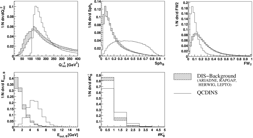
Figure 7: The event observables characterising the hadronic final state of $I$-induced processes in DIS at HERA providing good instanton separation along with small systematic uncertainties. Shown are simulations of $I$-processes (QCDINS) and of standard DIS background. The band indicates the uncertainty due to different QCD models. The observables are explained in text.

Starting with 35 observables based on the hadronic final state the best 12 were chosen by calculating the discriminant with all 2-combinations (pairs) of the initial observables and taking those observables which provide a high separation power $S=\epsilon_{s}/\epsilon_{b}$ demanding an efficiency for instantons of $\epsilon_{s}=10\%$. The number of considered observables is further reduced by calculating all 5-combinations and selecting those with highest separation power and a small systematic variation of the background. The systematic uncertainty was obtained by using four standard DIS-MC simulators [18] which were tuned to data on representative hadronic final state quantities, in the range $Q^{2}>100\,\mathrm{GeV}^{2}$ at HERA [19]. The observables forming the best combination are shown in figure 7. These are: the reconstructed virtuality of the quark entering the I-subprocess $Q{{}^{\prime}}_{\rm rec}^{2}$, the sphericity of the particles in the I-Band in their rest system ${\rm Sph}_{B}$, the second Fox-Wolfram moment [20] ${\rm FW}_{2}$ of these particles and the event shape observables $E_{\rm out,B}$ which is the projection of the particle transverse momentum onto the axis that makes this quantity maximal [21] and finally the number of charged kaons in the I-Band (see [22] for a detailed description of the observables).

The separation power for $\epsilon_{s}=10\%$ is $S=126$. In figure 8a the expected number of I-induced events in DIS at HERA and the number of background events is shown as a function of the discriminant $D$, for a data sample of an integrated luminosity of $100\,{\rm pb}^{-1}$. Only the signal region defined by $D>0.9$ is shown. The luminosity is comparable to the one already collected by each of the HERA experiments H1 and ZEUS. An event sample can be isolated where half of the events are instantons while the I-efficiency is still 10%. The decreasing background model uncertainty in the signal region reflects the choice of observables with a minimum background uncertainty, which was possible due to the speed and flexibility of the PDE-RS method.

Figure 8: a) Number of events expected for an integrated luminosity of $100\,{\rm pb}^{-1}$ as a function of the discriminant for instanton-induced and standard DIS processes. Only the signal region with $D>0.9$ is shown. b) Separation power $S$ at $\epsilon_{s}=10\%$ for different relative box widths and different numbers of events in the binary trees.

To reduce the number of parameters for the box size, the ratios of the box edge lengths were fixed by defining a box which contains most of the events and letting $V$ be a scaled version of this large box. The projections onto these box edges are shown in figure 7. The variation of the result depending on the size of $V$ is shown in figure 8b. The behaviour is similar to the one in the toy-model: The separation increases for smaller boxes with the number of events that populate the search trees, while for larger boxes this difference vanishes. The width of the plateau increases with the number of events in the classification tree. If the data sample is large enough, the width of the plateau spans one order of magnitude. This allows to use only an approximate size parameter which reduces the need for fine tuning, if a large enough Monte Carlo data sample is available.

In addition a comparison with a single hidden layer feed forward NN was done. Several network architectures were tried. The network performing best had 3 layers with 100 hidden nodes. It reached a separation of $S=116$ at an I-efficiency of 10%, being slightly worse than the PDE-RS method. To get this good performance the high numbers of nodes was mandatory. Training the net was rather time consuming and a lot of human intervention was needed to adjust the training parameters.

6 Conclusions

For the examples covering different basic problems appearing in High Energy Physics data analyses the presented new classification algorithm based on range searching (PDE-RS) has a discrimination power which is comparable to the one provided by Neural Networks. However, the PDE-RS method needs less computation time, is more transparent and is rather insensitive to the choice of the free parameters that need to be set manually. Moreover the classification error can be easily evaluated. For complex cases the speed of the algorithm allows to carefully choose the best combination of observables which give the best separation and for which the observables and their correlations are well described by the simulations. The PDE-RS method is therefore a powerful tool to find a small number of signal events in the large data samples expected at future colliders. It is particularly suited for hadron colliders where the background is large and the correct background description is difficult.

7 Acknowledgements

We would like to thank Prof. V. Blobel for making us aware of the range search algorithms and for many discussions helpful to develop a method suitable for High Energy Physics applications. A. Ringwald and F. Schrempp we would like to thank for many years of fruitful collaboration on investigating search strategies for I-induced processes in DIS. Many thanks also for initiating first ideas to apply multi-variate discrimination techniques for I-searches. Finally we would like to express our gratitude to P. C. Bhat, V. Blobel, L. Holmström, C. Kiesling, D. Lelas and J. Zimmermann for comments on the manuscript.

References

- [1] P. C. Bhat, in: Proc. of the 8th meeting of the Division of Particles and Fields of the APS (DPF’94) (Albuquerque, USA, 1994); FERMILAB-CONF-94-261-E.
- [2] L. Holmström, S. R. Sain and H. E. Miettinen, Comp. Phys. Comm. 88 (1995) 195.
- [3] R. Raja, Phys. Rev. D 55 (1997) 2902.
- [4] P. C. Bhat, R. Gilmartin and H. B. Prosper, Phys. Rev. D 72 (2000) 074022.
- [5] C. M. Bishop, Neural Networks for Pattern Recognition, Clarendon Press (Oxford, UK, 1995) and references therein.
- [6] H1 Collab., C. Adloff et al., hep-ex/0205078; accepted by Eur. Phys. J. C.
- [7] ZEUS Collab. , Contributed paper Nr. 909 to the XXXI Int. Conf. of High Energy Physics, (Amsterdam, Netherlands, 2002).
- [8] J. L. Bentley, Comm. of the ACM, 18, (1975) 9.
- [9] J. L. Bentley and J. H. Friedman, Computing Surveys 11 (1979) 4.
- [10] R. Sedgewick, Algorithms in C++, Addison Wesley (Boston, USA, 1992) Chapter 26.
- [11] S. Towers, in: Proc. of the Advanced Statistical Techniques in Particle Physics Conference, (Durham, UK, 2002), Ed. L. Lyons.
- [12] A. Belavin et al., Phys. Lett. B 59, 85 (1975); G. ’t Hooft, Phys. Rev. D 14, 3432 (1976).
- [13] S. Moch, A. Ringwald and F. Schrempp, Nucl. Phys. B 507 (1997) 134; A. Ringwald and F. Schrempp, Phys. Lett. B 438 (1998) 217; A. Ringwald and F. Schrempp, Phys. Lett. B 459 (1999) 249.
- [14] A. Ringwald and F. Schrempp, in: Quarks ’94, (Vladimir, Russia, 1994) Eds. D. Yu. Grigoriev et al. (World Scientific, Singapore, 1995); hep-ph/9411217.
- [15] A. Ringwald and F. Schrempp, in: New Trends in HERA Physics 1999, eds. G. Grindhammer et al. (Tegernsee, Germany, 1999); hep-ph/9909338.
- [16] A. Ringwald and F. Schrempp, Comp. Phys. Commun. 132 (2000) 267.
- [17] T. Carli, J. Gerigk, A. Ringwald and F. Schrempp, in: Monte Carlo Generators for HERA Physics (Hamburg, Germany, 1999), Eds. A. Doyle et al., DESY-PROC-1999-02; hep-ph/9906441.
- [18] G.Ingelman, A. Edin and J. Rathsmann,Comp. Phys. Comm. 101 (1997) 108; H. Jung, Comp. Phys. Comm. 86 (1995) 147; L. Lönnblad, Comp. Phys. Comm. 71 (1992) 15; G. Marchesini et al., Comm. Phys. Comm. 67 (1992) 465.
- [19] N. Brook et al., in: Monte Carlo Generators for HERA Physics (Hamburg, Germany, 1999), Eds. A. Doyle et al., p 10; hep-ex/9912053.
- [20] G. Fox and St. Wolfram, Nucl. Phys. B149 (1979) 413.
- [21] M. Gibbs et al., in: Future Physics at HERA (Hamburg, Germany, 1996), Eds. G. Ingelman, A. deRoeck and R. Klanner, vol 1, p. 509.
- [22] B. Koblitz, Ph.D. Thesis, MPI-PhE/2002-07, DESY-THESIS-2002-015.