Other Atmospheric Neutrino Experiments

Abstract

The history and recent progress of atmospheric neutrinos are reviewed. An emphasis is placed on results from experiments other than Super-Kamiokande.

1 Introduction

The Super-Kamiokande experiment[1] has used their measurements of atmospheric neutrinos to persuasively and clearly demonstrate the existence of neutrino oscillations, with excellent agreement with the hypothesis $\nu_{\mu}\rightarrow\nu_{\tau}$. With lower statistics, other experiments have measured atmospheric neutrinos for a long time and continue to do so. In this paper, after reviewing the creation and measurement of atmospheric neutrinos, I discuss the history of atmospheric neutrinos along with two possible alternative scenarios. I then review the most recent results from Baksan, Soudan 2 and MACRO.

2 The Creation of Atmospheric Neutrinos

Atmospheric neutrinos originate from the decays of $\pi$’s, $K$’s and $\mu$’s produced when cosmic rays hit the atmosphere and interact. There are also a smaller number of neutrinos produced by the decay of charmed particles, $\tau$’s and other high mass particles, but their detection has not been demonstrated. $K$ and $\pi$ decay give mainly $\nu_{\mu}$’s while $\mu$ decay gives both $\nu_{\mu}$’s and $\nu_{e}^{\prime}s$. The $\mu$’s themselves come from $\pi$ and K decay, so at low energy (below 2 GeV where all of the muons decay before they hit the earth), the flux of each flavor neutrino $\phi(\nu_{\mu}+\bar{\nu}_{\mu}):\phi(\nu_{e}+\bar{\nu}_{e})$ occurs in the ratio 2:1. The experimental value for this ratio (in the absence of oscillations) for charged current interactions will vary from 2 for several reasons:

1. Containment differences between $\mu$ and e

2. $\nu_{\mu}$ charged current threshold

3. $\nu_{e}$ and $\bar{\nu}_{e}$ differences due to their different cross sections and the fact that $\mu^{+}/\mu^{-}$ ratio is about 1.2

4. Some additional $\nu_{e}$’s from $K^{+}_{e3}$ and $K^{0}_{e3}$ decays

5. Higher energy $\mu$’s hit the earth and lose most of their energy before decaying.

For detectors built to study proton decay, the first factor is the most important, and the ratio is under 2. For high energy neutrino telescopes, the last factor causes the ratio to increase to large values.

The density profile of the atmosphere affects the geometry of the source. The overburden, and hence the pressure, [2] goes as

$$X=X_{0}\exp{(-\rho gh/kT)}=X_{0}\exp{(-h/h_{0})}$$ (1)

where the latter expression is used to define the scale height $h_{0}$, which is about 8.4 km at sea level. Since T and hence $h_{0}$ depend on altitude, $h_{0}$ decreases to 6.4 km near the tropopause, where many atmospheric $\nu$ are created. Also, the air temperature induces seasonal variations of muon and neutrino fluxes. Muon seasonal variations are typically $\pm 2\%$, but since high energy neutrinos come primarily from $K$’s, this effect is small for high energy neutrinos. A bigger effect at low energy is the solar cycle variation, which occurs because the magnetic field of the solar wind prevents many low energy cosmic rays from reaching the earth’s location in the solar system.

If all neutrinos came from the same height in the atmosphere, there would be a strict relationship between the local neutrino zenith angle in an underground detector and the neutrino pathlength $L$ which is relevant for neutrino oscillation analysis. Those production height distributions vary with both neutrino angle and energy. A useful parameterization has been performed by Ruddick[3]. A comparison of his parameterization with a full Monte Carlo at two choices of energy and angle are shown in Figure 1.

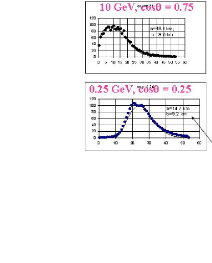
Figure 1: Production height distributions for two neutrino energies and angles.

3 Detection of Atmospheric $\nu$

Two classes of atmospheric neutrino events are considered in this paper. A neutrino may interact in an underground detector, or it may interact outside the detector and make a muon which is detected. Events of the first category include the contained events and partially contained events of Soudan 2, IMB and Kamiokande and the semi-contained events of MACRO. Events of the second category include the upward throughgoing $\mu$’s and stopping $\mu$’s of MACRO and Kamiokande and the horizontal $\mu$’s of KGF, Soudan 2 and Frejus. An attempt to catalog the world total of atmospheric $\nu$’s is given in Table 1. Only neutrino candidates which are background free or background subtracted have been included. It is clear that Super-Kamiokande dominates the total.

Experiment	Contained	$\nu$ induced $\mu$
CWI/SAND[4]	0	121
KGF[5]	100	229
NUSEX[6]	40	0
Soudan 1[7]	1	0
Frejus[8]	271	44
IMB[9]	935	624
Kamiokande[10]	557	372
Soudan 2[11]	561	73
LVD*	0	?
Baksan*[12]	0	801
MACRO[13]	285	940
AMANDA*[14]	0	204+
BAIKAL*[15]	0	44+
Subtotal	2750	3452
Super-Kamiokande[1]	12785	$\sim$ 1850

Table 1: Atmospheric neutrino event totals. The *’s represent experiments that are still taking data. The total, not including Super-Kamiokande is 6202 $\nu$ events

4 History

The first reported atmospheric $\nu$ was measured in the KGF experiment[5] using a set of telescope counters consisting of iron, flash tubes and scintillator. That telescope was operated on several levels of the KGF mine, but started at 7600 MWE level where the nucleon decay and monopole detectors were later built. The measured angular distribution in the latter detectors shows a clear separation between atmospheric $\mu$’s and $\nu$ induced $\mu$’s. This is shown in Figure 2. Eventually, 100 contained events and 229 $\nu$ induced horizontal $\mu$’s were measured at KGF.

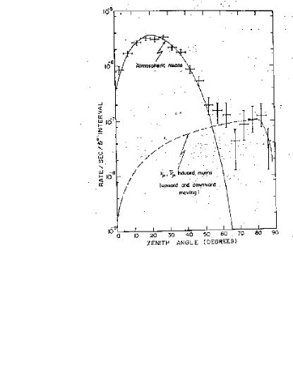
Figure 2: Zenith angle distribution of muons in KGF.

The first recorded atmospheric $\nu$ was measured on 23 February, 1965 in the South African Neutrino Detector (CWI/SAND) built by the Case-Western-Irvine Group.[4] Again, the signature for an atmospheric $\nu$ was the projected zenith angle. Due to the extreme depth of that detector (8890 MWE), the zenith angle where an atmospheric muon and neutrino induced muon can be clearly separated was about 50^o.

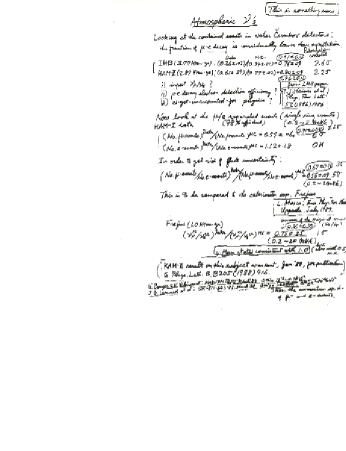
Figure 3: Koshiba’s slide from 1988 Fermilab Workshop.

More atmospheric neutrino data became available in the 1980’s from large detectors which were built to search for nucleon decay. The first hint of the atmospheric neutrino problem, which was also known as the “too few nu mu” problem came in the IMB1 data. They measured the number of delayed coincidences due to muon decays.[16] This distinguished $\nu_{\mu}n\rightarrow\mu^{-}p$ and $\bar{\nu}_{\mu}p\rightarrow\mu^{+}n$ followed by $\mu\rightarrow e\nu\bar{\nu}$ from $\nu_{e}n\rightarrow e^{-}p$ and $\bar{\nu}_{e}p\rightarrow e^{+}n$ events. They reported, “The simulation predicts 34% $\pm$ 1% of the events should have an identified muon decay while our data has 26% $\pm$ 3%. This discrepancy could be a statistical fluctuation or a systematic error due to (i) an incorrect assumption as to the ratio of muon $\nu$’s to electron $\nu$’s in the atmospheric fluxes, (ii) an incorrect estimate of the efficiency for our observing a muon decay, or (iii) some other as-yet-unaccounted-for physics.” It has turned out to be the latter.

To learn from an anomaly, there needs to be not only results inconsistent with expectation, but also someone to take it seriously and to carefully study alternative explanations. The first detailed evaluation of the atmospheric neutrino problem that I personally saw was a discussion by Koshiba at the 1988 New Directions in Neutrino Physics Fermilab Workshop. There he showed the transparency in Figure 3. He compared the “ratio-of-ratios” defined as

$$R=\frac{(\nu_{\mu}/\nu_{e})^{data}}{(\nu_{\mu}/\nu_{e})^{MC}}$$ (2)

for several experiments and several different methods. The Water Cerenkov Detectors could measure the ratio two different ways, with muon decays and with ring fits. The initial measurements of the iron calorimeters, Frejus and NUSEX got higher values consistent with unity, but NUSEX had quite low statistics, and even Frejus had a noticeable $\nu_{\mu}$ deficit if one looked only at the fully contained events. The period 1988-1995 was the period of the “ratio-of-ratios” or the “atmospheric neutrino anomaly”. Several attempts to understand the anomaly either as a systematic effect or as an error in the atmospheric neutrino Monte Carlos did not succeed.

In 1994, the Kamiokande experiment[10] showed another data set, their Multi-GeV data. In the Multi-GeV data, not only was there a deficit of $\nu_{\mu}$, and a value of $R$ below unity, but there was also a zenith angle distribution consistent with neutrino oscillations. By contrast, their zenith angular distribution for the Sub-GeV contained events was flat. This suggested a higher value of $\Delta m^{2}$ than currently seen. It has been widely noticed that the parameter space plots ( in $\sin^{2}(2\theta)$ and $\Delta m^{2}$) for Kamiokande and Super-Kamiokande did not overlap. It is interesting to compare the zenith angle plots of Kamiokande data and Super-Kamiokande data for Sub-GeV and Multi-GeV, e and $\mu$. In such a comparison, no data points disagree by much more than one sigma. The disagreement in parameter space comes about in the fits. It is worthwhile to point out that fits for $\Delta m^{2}$ are not gaussian, and that it is possible to have multiple solutions similar to the degeneracies now facing experiments planning to measure $\theta_{13}$ and $\delta_{CP}$.

5 Gedanken History

Let’s imagine the status of atmospheric neutrinos for two scenarios in which history had been different.

The largest underground experiments for nucleon decay and magnetic monopole detection were motivated by Grand Unified Theories. In the absence of such motivation, the only experiments which measured atmospheric $\nu$’s would have been CWI/SAND, Baksan and LVD. Solar neutrino experiments would have proceeded on their same time scale (or even faster). There would likely have been a greater interest in the reported neutrino oscillation signature from the LSND experiment[17], as well as in proposed short and intermediate baseline experiments such as BNL to Long Island, CERN to JURA and the never-realized Fermilab COSMOS experiment. The solar neutrino results in the 80’s and 90’s might have motivated some forward thinking individuals to propose a large underground experiment to measure atmospheric neutrinos. There would probably have not been great enthusiasm for such an experiment, most sensitive to large mixing angles, until after the SNO results in 2002. Even then, I think it would have been a hard project to realize.

History would also have been quite different if the Super-Kamiokande accident had happened during its first fill in 1995. Confidence in rebuilding the detector might not have been possible in the absence of the 5 successful years of running the detector. The K2K run would not have taken place. MINOS, which had already been approved, would have continued to plan with its high energy beam, most sensitive to larger values of $\Delta m^{2}$. New data from MACRO and Soudan 2 would be tending to support lower values of $\Delta m^{2}$, but given the non-gaussian (and hence unintuitive) nature of $\Delta m^{2}$ fits, the situation would be fairly confused, which would have lead skeptics to doubt conclusions about atmospheric neutrino oscillations. The latest Soudan 2 and MACRO data analyses would be quite relevant in trying to sort out the situation.

6 Recent Results from Baksan

The Baksan Underground Scintillator Telescope has been taking data since the 1980’s, with its four layers of scintillator detectors under a mountain at a minimum 850MWE. At Neutrino 2000, they reported on data from December 1978 to January 2000, corresponding to 15.7 years of livetime. They measured 801 upward $\mu$’s with an expected rate (in the absence of oscillations) of 941.6. The zenith angle distribution was not in close agreement with oscillation fits, though the rates agree with other experiments. They now have about another 10% increase in statistics, but will not present a new analysis until next year or later, when the increase is 25% or more.

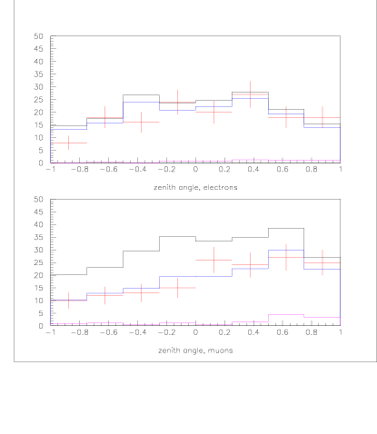
Figure 4: Zenith angle distributions in Soudan 2 for e (top) and $\mu$ (bottom). Shown are data points, and histograms with and without oscillation fits. A small background is also shown.

7 Recent Results from Soudan 2

Soudan 2 is a very fine-grained drifting calorimeter with drift cells located in a honeycomb pattern of iron plates. Since Neutrino 2000, the Soudan 2 experiment has finished taking data. It finished in July 2001 with a total 5.91 fiducial kt-year for contained event data. Details of the current status of Soudan 2 analyses for atmospheric neutrinos can be found in Reference [18]. A recent feature of the Soudan 2 data analysis is that a 15% problem with the electron energy scale has been resolved. Data analysis now includes the partially contained events, and parameter space fitting is done with a Feldman-Cousins[19] type of analysis. A feature of Soudan 2 which has been exploited for some time is the ability to measure recoil protons, which appear in this very fine-grained detector as short, straight, heavily ionizing tracks from the main vertex. The events which have an identified recoil proton allow the neutrino zenith angle, and hence the $L$ relevant for $L/E$ analyses, to be reconstructed with much greater accuracy. Soudan 2 defines its high-resolution sample to be the high energy quasi-elastics, the low energy quasielastics with a recoil proton and the high energy multiprongs. The zenith angle distributions of the electrons and muons are shown in Figure 4 and the $L/E$ distribution in Figure 5.

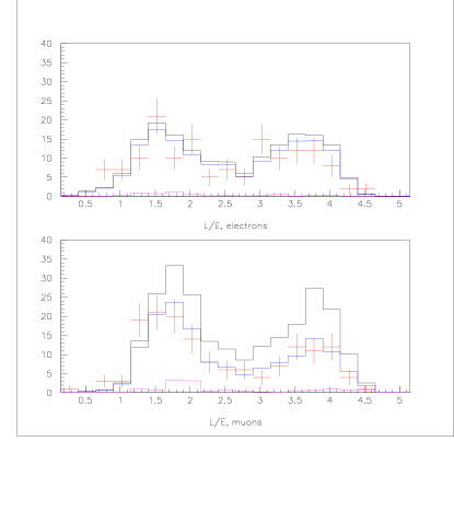
Figure 5: $\log_{10}$ $L/E$ distribution in Soudan 2 for e(top) and $\mu$(bottom). The histograms have the same meaning as in Figure 4.

The Feldman-Cousins analysis involves calculating the likelihood of the data as function of $\sin^{2}(2\theta)$ and $\Delta m^{2}$ parameters for the data and for Monte Carlo data. A confidence level diagram is calculated from the difference in log-likelihood. This is shown in Figure 6. The best fit occurs at a value of $\Delta m^{2}$ = 0.010 $eV^{2}$ and $\sin^{2}(2\theta)$ = 0.97. It should be noted that the valley near the best fit is quite flat, particularly towards lower values of $\Delta m^{2}$.

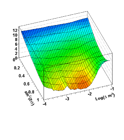
Figure 6: Likelihood surfaces for Soudan 2 data.

8 Recent Results from MACRO

The MACRO experiment is a large area detector in the Gran Sasso laboratory, consisting of 3 towers of scintillation counter and 14 horizontal planes of streamer tubes. MACRO completed its data taking in the last two years, finishing with 5.52 live years in December 2000. With excellent timing, MACRO was able to separate upward and downward going events, but the trigger gave poor acceptance for horizontal muons. The categories of events in MACRO were 809 + 54 [background subtracted + background] (1122 [Monte Carlo]) upthroughgoing muons, 154 +7 (285) internal upgoing (IU) events, and 262+10 (375) upgoing stopping muons (UGS) plus internal downgoing muons (ID).

The shapes of the zenith angle distributions of the MACRO event samples are sensitive to neutrino oscillations. For the throughgoing muons, the ratio of events with $-1<\cos\theta<-0.7$ to events with $-0.4<\cos\theta<0$ can be used to distinguish $\nu_{\mu}\rightarrow\nu_{\tau}$ from $\nu_{\mu}\rightarrow\nu_{s}$ oscillations because of a matter effect[20]. The $\nu_{\tau}$ has a neutral current interaction in matter while the $\nu_{s}$ does not, and this difference in interaction leads to a different expected oscillation probability. Based on the ratio test, $\nu_{\mu}\rightarrow\nu_{s}$ oscillation has only a 0.033% probability of fitting the data, and is disfavored by $>99\%$CL compared to the best fit $\nu_{\mu}\rightarrow\nu_{\tau}$ oscillation.

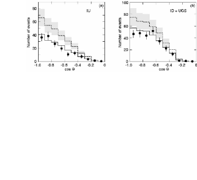
Figure 7: Angular Distributions of MACRO low energy neutrino data, along with expected shapes with and without oscillations. The shaded area shows the uncertainty of the flux estimate.

The angular distribution of the MACRO low energy data is given in Figure 7. For both the IU and UGS+ID data sets, the data falls below the expectation (without oscillations), even taking into account the normalization uncertainty of the expectation. And together with the throughgoing data, they form an acceptable fit to the same neutrino oscillation parameters.

MACRO has also recently shown new results which use muon energy in the analysis.[21] The muon energy is not measured calorimetrically or magnetically. However, the multiple scattering in the detector is dependent on the energy on average in a known way. The projected displacement from a straight line fit for a relativistic muon is inversely proportional to the muon momentum. They have obtained an improvement of the space resolution using the limited streamer tubes in drift mode, and through an analysis of the multiple scattering, obtained an energy estimate on a muon by muon basis. With that energy, and the zenith angle which gives an estimate of the neutrino flight path, they have made an $L/E_{\nu}$ distribution. This is shown in Figure 8 along with the expected distribution for the best fit oscillation parameters.

The allowed parameters ($\Delta m^{2}$, $\sin^{2}(2\theta)$) according to the low energy and high energy MACRO analyses are shown in Figure 9 along with the analysis of Soudan 2. The results of both experiments agree with each other and with Super-Kamiokande. Each experiment also rejects the null hypothesis of no oscillations with high probability.

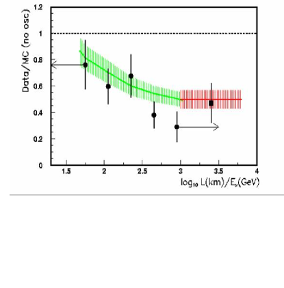
Figure 8: $L/E$ distribution of MACRO data based on multiple scattering estimation.

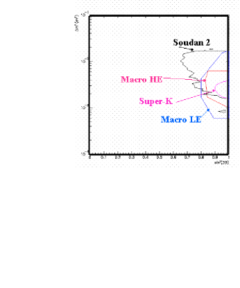
Figure 9: Comparison of parameter space estimates for MACRO and Soudan 2

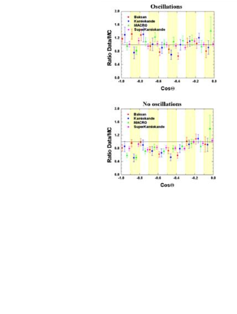
Figure 10: Comparison of zenith angle distributions of throughgoing muons

9 Summary

There are several experiments besides Super-Kamiokande which collectively have observed atmospheric neutrinos. Analyses of these data agree with the essential Super-Kamiokande result: neutrino oscillations are required to account for the data. Taken as a whole, contained event data from IMB, Kamiokande, Soudan 2, and Frejus all agree with a 30%-40% deficit of $\nu_{\mu}$ induced events, and also agree with the higher statistics Super-Kamiokande results. New features from Soudan 2 data strengthens that conclusion. Soudan 2 now has an up/down difference in its contained events which is statistically significant, and supports the region of parameter space found by Super-Kamiokande. With its recoil proton identification and good angular resolution, Soudan 2 has the resolution, but not the statistics, to see the “reappearance” in the $L/E$ distribution.

Detailed analyses of $\nu$ induced muons support a similar conclusion. All experiments see a deficit of $\nu_{\mu}$ consistent with the Super-Kamiokande observations, and an angular distribution which is more consistent with the neutrino oscillation hypothesis than with the null hypothesis, as shown in Figure 10, a comparison of data from Baksan, Kamiokande, MACRO and Super-Kamiokande.[22] It is interesting to point out that the probability of the best fit for all four experiments is less than 30% each, so it is worthwhile to continue to investigate whether some aspect of the physics is not being modeled correctly.

It is left to another speaker at Neutrino 2002 to consider the proposals for future atmospheric neutrino oscillation projects.[23] However, I want to make a general observation, that much of the progress in atmospheric neutrinos has come from experiments that were designed to search for GUT predicted nucleon decay. The motivation for much larger experiments to continue that search is quite strong, and we as a field have the technical means to accomplish such a search in our lifetime. I hope that search takes place. If it does, a much firmer understanding of atmospheric neutrinos will be an inevitable outgrowth of such an effort.

References

- [1] Y. Fukuda et al., Phys.Rev.Lett. 81 (1998) 1562; also M. Shiozawa, these proceedings.
- [2] Thomas Gaisser, “Cosmic Rays and Particle Physics” Cambridge University Press, 1990.
- [3] K. Ruddick, “New Parameterizations of atmospheric neutrino production heights”, PDK779, November 2001, unpublished.
- [4] Reines et al., Phys. Rev. Lett. 15, (1965) 551; Crouch et al., Phys. Rev. D18, (1978) 2239.
- [5] C. Achar et al., Phys. Lett. 18, (1965) 196; also N. Mondal, private communication.
- [6] Aglietta et al., Europhy. Lett., 7 (1989) 611.
- [7] D. Ayres, private communication.
- [8] K. Daum et al., Z. Phys. C66, (1995) 417.
- [9] D. Casper et al., Phys. Rev. Lett. 66 (1991) 2561; and R. Becker-Szendy et al., Phys. Rev. D46 (1992) 3720.
- [10] K.S. Hirata et al., Phys. Lett. B205, (1988) 416; K.S. Hirata et al., Phys. Lett. B280, (1992) 146.
- [11] To be published by Soudan 2.
- [12] S. Mikhaev, private communication.
- [13] M. Abrosio et al., Phys. Lett. B434 (1998) 451; also M. Spurio, these proceedings.
- [14] D. Cowen, these proceedings.
- [15] G. Domogatsky, these proceedings.
- [16] T. Haines et al., Phys. Rev. Lett. 57 (1986) 1986.
- [17] Aguilar et al., Phys.Rev. D64 (2001) 112007.
- [18] M. Sanchez, these proceedings.
- [19] G. Feldman and R. Cousins, Phys.Rev. D57 (1998) 3873.
- [20] T. Montaruli, 2001 ICRC Proceedings, 1069.
- [21] M. Ambrosio et al, physics/0203018, (2002).
- [22] S. Mikhaev, private communication.
- [23] T. Tabarelli de Fatis, these proceedings.