The Hadron Hose: Continuous Toroidal Focusing for Conventional Neutrino Beams

Abstract

We have developed a new focusing system for conventional neutrino beams. The “Hadron Hose” is a wire located in the meson decay volume, downstream of the target and focusing horns. The wire is pulsed with high current to provide a toroidal magnetic field which continuously focuses mesons. The hose increases the neutrino event rate and reduces differences between near-field and far-field neutrino spectra for oscillation experiments. We have studied this device as part of the development of the Neutrinos at the Main Injector (NuMI) project, but it might also be of use for other conventional neutrino beams.

1 Introduction

Figure 1: Schematic layout of the NuMI neutrino beamline, showing the locations of the target, focusing horns, decay volume, and steel and earth shielding in front of the near MINOS detector. Two sample pion trajectories, are shown. Soft pions tend to enter the decay volume at large angles, while stiff pions enter at smaller angles.

The Hadron Hose is a current-carrying wire used to instrument the decay volume of a conventional neutrino beam with a toroidal focusing field for a sign-selected meson beam. Conventional neutrino beams are tertiary beams, with the primary proton beam producing $\pi$ and $K$ meson secondaries in a target. Beamline elements downstream of the target, called horns [1], produce a toroidal magnetic field to sign- and momentum- select the mesons, focusing them toward an evacuated or Helium-filled volume, where the mesons decay into the tertiary neutrino beam. Steel and earth shielding absorb remnant protons, mesons, and muons at the end of the decay volume (see Figure 1).

In conventional neutrino beams to date [2, 3, 4, 5, 6, 7, 8] the mesons freely propagate through the decay volume. The toroidal field of the Hadron Hose provides continuous focusing of the secondary meson beam throughout the decay volume. Mesons spiral around the hose wire and are drawn away from the decay volume walls where they might interact before decaying. A pion orbit in the NuMI beamline with the Hadron Hose is shown in Figure 2. The spiraling motion randomizes the decay angles of the mesons, which reduces the need to model detector and beamline acceptances in Monte Carlo calculations of the expected neutrino fluxes at the detectors.

Figure 2: Sample orbit of a 10 GeV pion in the NuMI beamline including the hadron hose. The toroidal field of the hose wire captures the pion in orbit around the wire. The orbit randomizes the decay angle between the pion direction and the direction of neutrinos that reach the MINOS detectors.

Toroidal magnetic fields have been used for plasma beams [9, 10] and the possibility of using toroidal fields to focus charged particle beams was noted by Van der Meer [11, 12]. In this article, we study the utility of such a focusing system for neutrino beams and the technical feasibility of placing such a wire in an evacuated region with high particle fluences. While we have developed this device for the Neutrinos at the Main Injector (NuMI) project, such a system might be of utility at future neutrino facilities such as the JHF [13] or conventional neutrino “super beams” [14, 15, 16].

This article procedes as follows: We discuss the focusing properties of the hose in Sections 2 - 3. Sections 4-7 present the mechanical and electrical design which was proposed for NuMI. Sections 8 through 12 discuss some of the hardware studies to demonstrate that the hose wire can survive in the radiation field of a neutrino beamline without significant failure of wire segments. Section 13 concludes.

2 NuMI Beamline

For NuMI, 120 GeV protons will be extracted from the Main Injector [17] and focused downward by 58 mRad, to strike a 0.94 m long graphite target. The bunch length is $8.6~{}\mu$sec, and the cycle time $1.87$ sec. The beamline is designed for $3.7\times 10^{13}$ protons/pulse and $3.8\times 10^{20}$ protons/year.

NuMI will have two focusing horns [17] pulsed at 200 kA after the target. The secondary hadrons enter a 675 m long, 1 m radius evacuated decay volume. MINOS [18] is a 2-detector neutrino experiment. A 980 ton near detector measures the neutrino energy spectrum and rate produced at Fermilab. A 5400 ton far detector is located in the Soudan mine in Minnesota, 735 km from Fermilab. The NuMI beam can be adapted to produce a low ($E_{\nu}^{peak}\sim 3$ GeV), medium ($E_{\nu}^{peak}\sim 6$ GeV), or high ($E_{\nu}^{peak}\sim 12$ GeV) energy neutrino event spectrum. Figure 3 shows the expected spectra in the two detectors for the low-energy and high-energy beam options assuming no new physics resulting in neutrino disappearance. In Figure 3, the vertical axis is the number of expected charged current neutrino interactions expected per kiloton of detector mass per $4\times 10^{20}$ protons on target ($\sim$1 NuMI year).

The neutrinos in the peaks of the spectra of Figure 3 come from pions focused by the horns, whereas the neutrinos in the high energy tail come from poorly focused pions (pions that travel through the necks of the horns). The high energy tail is nonetheless important to the experiment because it provides us a control sample to demonstrate a region without oscillation effects. It is important to make the best prediction of the far-field energy spectrum to search for any kind of spectral distortions.

It is desirable to have the neutrino energy spectra at the two detector sites as similar as possible so that the near detector site strongly constrains the calculation of the spectrum at the far site. Any relative difference observed at the far detector is evidence for new physics such as neutrino oscillations. In practice, the two detector spectra are not identical: the vastly different solid angles subtended by the two detectors results in an energy-dependent acceptance difference. This difference is evident in the neutrino spectra of Figure 3.

Figure 3: Neutrino energy spectra in the far and the near ($\times 10^{-6}$) MINOS detectors, computed without (above) and with (below) the Hadron Hose. The left plots are for the NuMI low-energy beam and the right are for the high energy beam.

The acceptance difference between the two detectors is accounted for in the “far-to-near ratio”, which is the factor by which the near detector spectrum must be multiplied to predict the far detector spectrum. It is defined as:

$$N_{\mbox{far}}^{i}=\mathcal{R}_{FN}N_{\mbox{near}}^{i}.$$ (1)

where $N_{\mbox{near}}^{i}$ is the observed number of events in the $i^{\mbox{th}}$ energy bin in the near detector, and $N_{\mbox{far}}^{i}$ is the predicted number of events in the $i^{\mbox{th}}$ bin in the far in the absence of new physics. Uncertainties in the calculation of $\mathcal{R}_{FN}$ lead to systematic uncertainties in the predicted far detector spectrum which limit the ultimate reach of physics searches.

The calculation of $\mathcal{R}_{FN}$ is complicated by the extended length and finite aperture of the neutrino beam geometry. If the neutrinos were produced from a point source, then $\mathcal{R}_{FN}$ could be estimated by $\mathcal{R}_{FN}=Z_{near}^{2}/Z_{far}^{2}$, where $Z_{near}$ ($Z_{far}$) is the distance from the target to the near (far) neutrino detector. Considering that neutrino beamlines are an extended source, one could weight this extrapolation factor by the pion lifetime along the length of the decay tunnel:

$$\mathcal{R}_{FN}={{\int_{z=0m}^{z=725m}e^{-\frac{0.43m_{\pi}z}{E_{\nu}c\tau}}{1\over(Z_{far}-z)^{2}}dz}\over{\int_{z=0m}^{z=725m}e^{-\frac{0.43m_{\pi}z}{E_{\nu}c\tau}}{1\over(Z_{near}-z)^{2}}dz}}$$ (2)

where the integral is over the length of the decay tunnel (725 m in the case of the NuMI beamline) and the substitution $E_{\pi}\sim E_{\nu}/0.43$ has been made.

Figure 4: The Far-over-Near ratio (F/N) calculated for the NuMI low energy beam using several predictions [24, 25, 26, 27, 28] for the production of hadrons in the NuMI target. Shown is the prediction without (upper plot) and with (lower plot) the hadron hose in the low-energy (left) and high-energy (right) beams. The dotted line is the result of the simplified calculation of the far-over-near ratio from Equation 2.

However, even this estimate of the near-far extrapolation is a simplification: not all decaying pions produce neutrinos within the finite acceptances of the two detectors and not all pions are able to decay before interacting along the decay pipe walls. Furthermore, the correct relation between the pion and neutrino energy is

$$E_{\nu}=\frac{0.43E_{\pi}}{1+\gamma^{2}\theta^{2}}$$ (3)

where $\gamma$ is the pion relativistic boost and $\theta$ is the decay angle of the pion. In fact, because low-momentum pions tend to enter the decay volume at wider angles and decay far upstream in the decay volume, while high-momentum pions tend to propagate much further, the acceptance of the near detector for high momentum neutrinos is larger than for low-momentum neutrinos. The acceptance correction $\mathcal{R}$_FN given in Equation 2 is incorrect in an energy-dependent manner because of the correlation in Equation 3. A more detailed extrapolation of the measured near spectrum to the far detector requires a Monte Carlo calculation which tracks secondary hadrons produced in the target through the beamline optics. A comparison of the naive calculation of Equation 2 to a GEANT [27] simulation of the NuMI beamline is shown in Figure 4.

3 Hadron Hose

The Hadron Hose consists of a wire at the center of the decay tunnel and carries a 1000 A peak current pulse. The current provides a toroidal magnetic field which continually focuses positive particles back toward the center of the decay pipe. A typical meson executes 2-3 orbits around the wire over the length of the decay pipe.

The hadron hose contributes three essential features. First, $\pi$’s and $K$’s that otherwise diverge out to the decay pipe walls and interact before they decay are given a restoring force back to the decay pipe center. Thus, $\pi$’s/$K$’s travel farther and have a greater chance to decay, so the neutrino event rate in the far detector is increased (see Table 1). Second, the pion decay distribution along the beamline direction more nearly follows a simple exponential, which reduces the difference in acceptance of the near detector to low-momentum vs. high-momentum pions. Thus, the extrapolation factor $\mathcal{R}$_FN more closely follows that given by the pion lifetime in Equation 2, as can be seen in Figure 4. Third, the pion orbits effectively randomize the decay angle between the pion direction and the neutrino that hits the MINOS near and far detectors. This randomization washes out the kinematic correlation between neutrino energy and decay angle in Equation 3, which otherwise always produces a softer spectrum in the near detector than the far detector. The difference is especially visible at the high energy edge of the high energy beam in Figure 3. The randomization is a larger effect for the high energy beam because the Lorentz boost at high energy otherwise increases the sensitivity to the decay angle in Equation 2. The effect is also demonstrated in Figure 5, which plots the ratio of neutrino energies in the near and far detector that would arise from the decay of a given pion in the low-energy or high-energy NuMI beam configurations.

Figure 5: The difference in the energy of the neutrino that a given pion would emit toward the far detector to that it would emit toward the near detector in NuMI/MINOS (see text) in the low-energy (left) and high-energy (right) beams, normalized to the near detector energy.

Beam	Events in peak	Overall Events
LE	261	474
LE-HH	327	732
HE	2694	2745
HE-HH	2870	2983

Table 1: Charged current event yields in the far MINOS detector in the low and high energy beam configurations, with and without Hadron Hose. The peak refers to the regions $E_{\nu}<$6 and 30 GeV, for low and high energy beams, while overall refers to $E_{\nu}<40$ GeV. The units are events per kiloton of far detector mass per $3.8\times 10^{20}$ protons on target.

By minimizing acceptance effects of the detectors to the beam, the hose reduces the experiment’s sensitivity to input data to the Monte Carlo. The largest systematic uncertainty in $\mathcal{R}_{FN}$ for NuMI are the cross sections for production of $\pi$’s/$K$’s in the target, $d^{2}\sigma/dx_{F}dp_{T}$. These have been measured [19, 20, 21, 22, 23], but gaps in these data sets in the $x_{F}$ and $p_{T}$ range relevant for NuMI, 10-20% disagreements between data sets, and systematic uncertainties in scaling these invariant cross sections to the NuMI beam energy and target material complicate efforts to model or parameterize the data for all $x_{F}$ and $p_{T}$. Using several parameterizations [24, 25, 26, 27, 28], 20-30% variations are found in neutrino flux predictions for the near and far detectors, and more importantly, up to 5% variations are predicted in the F/N ratio (see Figure 4). These variations are reduced with hose focusing.

Besides minimizing the experiment’s sensitivity to variations in pion productions cross sections, the Hadron Hose loosens accuracy criteria for other beamline components. For NuMI, the potential benefits include increasing the allowed eccentricity of the inner conductor of the first focusing horn from $<$0.08 mm at its neck position to $<$0.12 mm if hose focusing is implemented. In addition, the spatial alignment of the first horn transverse to the beamline is relaxed from $\pm 0.8$ mm to $\pm 1.0$ mm. Relative current variations between the two horns can be as large as $\pm 1.5$% (c.f. $\pm 1.0$%). Finally, the alignment of the NuMI decay pipe, previously required to be within 2 cm all along its 675 m length, would be relaxed to 3 cm.

Figure 6: The composition of neutrino species in the NuMI beam, with and without the hadron hose in the NuMI low-energy beam.

The Hadron Hose alters the backgrounds from $\overline{\nu}_{\mu}$, $\nu_{e}$, and $\overline{\nu}_{e}$ in the beam, as shown in Figure 6. The $\overline{\nu}_{\mu}$ backgrounds, which come from $\pi^{-}\rightarrow\mu^{-}\overline{\nu}_{\mu}$ decays, are reduced because the hose field defocuses $\pi^{-}$. The $\nu_{e}$ and $\overline{\nu}_{e}$ backgrounds are enhanced because $\mu^{+}$ daughters from $\pi^{+}$ decay are also focused by the hose field. In the case of NuMI, the factor of 2 increase in $\nu_{e}$ does not have a serious impact on $\nu_{\mu}\rightarrow\nu_{e}$ searches, since the putative signal would also go up by a factor of 30%, so signal/$\sqrt{\mbox{background}}$ is unchanged. For other experiments, the increase might be less because the NuMI decay pipe is quite long.

A Hadron Hose could also be designed to operate at currents of 1.5, 2.0, or even 4.0 kA. Such a design would be more ambitious than the NuMI proposal, requiring faster current power supplies for a shorter current pulse with equivalent $i^{2}r$ heating, or perhaps using several parallel wires running down the decay pipe. We found that a 2 kA current produces 20% more neutrinos in the NuMI low-energy peak than a 1 kA hose. The 2 kA hose doubles the ’high energy tail’ of the beam, however, so such an ambitious design would be more appropriate for a future, off-axis beamline where the high energy tail is suppressed. In any case, a 1 m radius decay pipe with the active focusing of the hose at 1 kA produces the same flux as does a beamline with a passive 2 m radius decay volume, and at a reduced cost.

4 Hose Wire Material Requirements

The choice of wire radius and material must be optimized for several considerations. First, larger radius wire tends to reduce neutrino event rates because of pions scattering in the wire. Second, larger wire can be better cooled in the near-vacuum of the decay pipe because both radiative and gas cooling grow with surface area of the wire. Furthermore, the heating of the wire is less for larger radius wire because the electrical resistance is reduced and so is $i^{2}r$ electrical heating. Third, while higher conductivity metals such as Copper improve electrical resistivity, low $Z$ is desirable to reduce pion scattering and neutrino event rate losses. We have chosen Aluminum alloy 1350, whose conductivity is $\approx 80\%$ that of Copper, and a radius of 1.15 mm, as discussed in this section. The subject of the following sections will be to demonstrate that this wire, when anodized to improve its emissivity, can survive the environment of the NuMI decay tunnel.

Figure 7: Monte Carlo predictions of the effect of pion interactions in the wire material on the neutrino event rate. Shown is the neutrino event rate in the MINOS far detector for a hose wire made of ’vacuum’ and for several choices of metals (NuMI medium-energy beam).

Figure 8: Monte Carlo predictions of the effect of the wire radius on the neutrino event rate. The simulation assumed an Aluminum hose wire and was simulated for the NuMI medium-energy beam.

To study the effects of wire material, simulations were made using no wire material, as well as aluminum, copper and tungsten. The charged-current (CC) event spectrum at the far detector calculated under these conditions are compared in Figure 7. The addition of the material results in a 3-6% decrease in the event rate below 10 GeV. Figure 7 also shows the change in the $\nu_{\mu}$ CC event rate at the far detector as a function of the atomic number of the wire material. In each case the wire radius was 2.8 mm. As much as a 9% decrease in the event rate below 12 GeV is seen for the highest $Z$ material.

The change in event rate is plotted in Figure 8 as a function of wire radius. The event rates are compared to simulations using no wire material. All simulations used aluminum wire. The event rate below 6 GeV is most strongly affected by the wire radius with roughly a 5% decrease at a radius of 1.4 mm. To reduce the loss of neutrino events due to scattering in the wire material, we chose a wire radius of 1.15 mm.

5 Hose Mechanical Design

The proposed design is to build 72 sections of wire, each 8.94 m in length and each of which is an independent circuit (see Figure 9). In this way, the voltage drop across a wire segment is reduced and the potential risk is reduced to the loss of a single segment in the event of a wire failure. In addition to the 72 segments, a 2 m long segment at the beginning of the decay pipe acts as a partial shield for the rest of the hose from the fraction of the proton beam which does not react in the target. The 1.15 mm radius Aluminum 1350 alloy wire is anodized with a Type II aluminum oxide layer 17 $\mu$m in thickness to increase its emissivity. Each hose segment is separated by 20 cm from its neighboring segment.

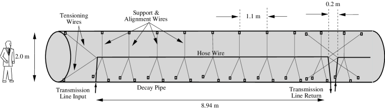
Figure 9: Schematic diagram of one hadron hose wire section, indicating support/alignment wires and tensioning wires.

The hose is supported at the center of the decay pipe by 0.5 mm diameter Invar support wires at intervals of 1.1 m along the hose wire’s length. Three Invar wires are plasma-welded to a small Invar loop which encircles the hose wire, constraining its position in the vertical and horizontal directions. Invar is chosen because of its low thermal expansion coefficient, so that it maintains hose wire alignment even with beam heating. The hose wire slides inside the loop with a 0.5 mm clearance, which allows the wire to elongate under heating without misalignment. The clearance contributes to the alignmnent error of the wire.

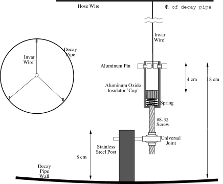
Figure 10: Diagram of the invar guide wires which support the hadron hose wire.

The Invar wire is mounted to the decay pipe wall with an insulating swivel mount, shown in Figure 10. A screw in this mount allows for fine positioning and alignment of the hadron hose wire. The insulator is chosen to be aluminum oxide ceramic and is located at the walls to reduce material at the center of the decay volume which can scatter hadrons. The choice of materials that can be used as the insulator is limited by radiation levels, ranging from 10¹¹ Rad/year expected at the decay pipe center to 10⁹ Rad/year expected at the walls of the decay pipe. A spring inside the lower two mounts tensions the Invar wire at 0.2 N. The inset to Figure 10 shows the three-fold Invar supports at one point along the hose wire’s length.

At the end of each hose wire segment, a 1.0 cm long, 1.0 cm outer diameter, 2.9 mm inner diameter, hollow aluminum cylinder is crimped on to the hose wire. Invar wires loop around this aluminum cylinder and are stretched to springs mounted on the decay pipe wall. These springs tension the hose wire to take up the expansion of the wire and reduce wire sag. The tensioning springs are mounted to the decay pipe wall using the same assembly as the guide wires. Since gravitational sag of the wire is a form of misalignment, the 1.1 m spacing between guide wire supports suggests that the required tension can be derived from $\delta=480L^{2}/\sigma$, where $\delta\sim$2 mm is the wire sag, $L=1.1$ m, $\sigma$ is the wire tension per unit area in pounds per square inch (PSI), and the mass density for aluminum has been assumed. We find $\sigma~{}=~{}290$ PSI, or 2 lbs=0.9 N tension on a 1.2 mm radius aluminum wire.

The current is delivered through the decay pipe wall by a feedthrough constructed of zirconium oxide insulator and Swagelok compression fittings (see Figure 11). A pin passing through the hollow 1.9 cm diameter insulator is welded on the inside to the hose wire segment which is bent out to the decay pipe wall, and on the outside is welded to the transmission line. The insulator is sealed to the wall by a bulkhead Swagelok fitting welded to the wall, and is sealed to the pin with a 3/4”-to-1/4” Swagelok reducing union. A feedthrough is connected to each end of each 9 m long section.

Figure 11: Diagram of the electrical feedthrough at the ends of each wire segment.

The effect of misalignment of the Hadron Hose wire was tested in two manners. First, random error was studied by introducing random displacements of the wire ends in ($x,y$ and $z$) in the Monte Carlo simulation. RMS misalignment of the wire by 3 mm results in approximately a 2.5% decrease in the event rate at the far detector below 6 GeV, and grows to 7% for misaligments of 5 mm. We therefore chose a 2 mm misalignment tolerance. Second, systematic misalignmnents were studied by misaligning the entire hadron hose wire with respect to the central beam axis defined by the proton beam, target, and horns. In this case, we found that the pion beam orbits follow the misaligned hose direction. Thus, collinear offsets of the hose wire result in no change in the neutrino flux, while an angular misalignments actually result in an off-axis neutrino beam energy spectrum [30] for the on-axis detectors. Other systematic effects of shorter length scale, such as ’bowed’ placement of the hose wire along the decay tunnel, or even gravitational wire sag (see Figure 13), tend to result in neutrino flux loss similar to the random misalignments because of the similar length scale as the random misalignments studied.

The performace of the Hadron Hose has been simulated under various failure conditions. In the first study, a pessimistic failure rate of 10% of the wire segments was assumed and random segments were selected for failure. This failure rate causes roughly a 10% decrease in the near and far detector events rates. Simulations were also made assuming failure of the first two segments. As these segments receive the most beam heating they are perhaps more likely to fail. Failure of the first two segments results in roughly a 3% decrease in the event rate below 8 GeV. Robustness and the ability to operate with a few broken segments is important because the decay volume will become radioactivated, making replacement of a wire impossible.

6 Full Scale Prototype Section

We have built a 14 m long prototype of the NuMI decay pipe and instrumented it with a full-length hadron hose wire segment, as well as two dummy segments at either end. In addition to practicing installation procedures, we investigated whether the wire vibrated at all during electrical pulsing, given that the leads of adjacent hose segments could, in principle, exert forces on one another of $\mu_{0}I^{2}/2\pi r~{}\sim~{}2$ N. We observed the wire through an optical telescope during pulsing of the wire. No effect as large as our sensitivity of 25 $\mu$m was observed. Furthermore, the wire was observed to remain centered during various tests to simulate expansion of the wire under heating or creep: pulling on one end of the wire segment, the spring tensioning on the opposite end of the segment expanded, while the support/alignment wires kept the opposite end centered. The Invar loop which constrains the hose wire properly allowed the wire to slide along the beamline direction, but maintained radial alignment.

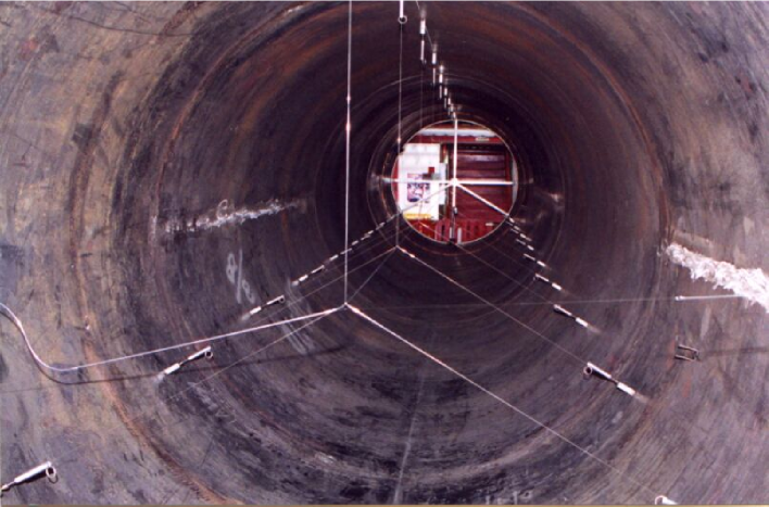
Figure 12: Photograph of the full-size NuMI decay pipe segment outfitted with a hadron hose segment.

The hose wire was aligned by first using a laser tracker to locate all of the support posts which were welded to the pipe walls. A 1/4” hole diameter at the top of each post provided a precision reference point. The laser tracker located all the posts within a 10 m span of the pipe, and was then moved down the pipe to survey an additional, overlapping 10 m span. These data were then used to define a set of coordinates for the center of each Invar support with respect to the tooling ball locations in the posts, and the Invar supports were set in place to these coordinates using the laser tracker. After sliding the wire through all the Invar support loops and attaching the tensioning springs, a stick micrometer was used to confirm the relative location of the hose wire to the tooling balls mounted on the posts. The results of the after-installation survey are shown in Figure 13. As can be seen, the horizontal displacements of the wire from the ideal centerline are within 1 mm, and in the vertical direction the supports are located to within 1 mm as well. In the vertical, the observed $\sim~{}2$ mm displacements of the wire from the centerline which occured between the invar suuports agree with our expectations for wire sag.

Figure 13: Results of the survey of the hose wire in the prototype section after installation. Measurements were made at each of the 9 Invar support locations and also halfway in between each pair of supports to observe wire sag.

7 Hose Electrical Design

The electrical design of the hadron hose must optimize for three factors. First, the current pulse of 1000 A must be long compared to the beam spill length (8.6 $\mu$sec for NuMI) and consistent from wire segment to wire segment. Second, the pulse must be fast to reduce $i^{2}r$ heating of the wire. Third, the pulse must be slow enough so that the inductive voltage drop does not cause voltage break down of the wire in vacuum. This section describes the electrical design that meets the voltage drop and heating requirements described in Sections 8 and 11.

7.1 Circuit Parameters

The design of the power supply and transmission line to deliver the current pulse to the hose wires is determined largely by the ciruit parameters for each segment. The current pulse will be of order 0.5 msec in duration each 1.8 sec, and runs down the wire and returns through the iron of the decay pipe wall.

The circuit inductance for the hose is dominated by the vacuum between the wire and the decay pipe. The inductance of the wire is $L_{wire}=\frac{\mu_{0}}{8\pi}=5\times 10^{-2}\mu{\rm henry/m}$. The inductance per meter of the vacuum space between the inner and outer conductors is

$$L_{vac}={\mu_{0}\over 2\pi}\ln({r_{pipe}\over r_{wire}})=1.34\times 10^{-6}{\rm henry/m}$$

for the radii $r_{wire}=1.2$ mm and $r_{pipe}=1$ m. The inductance per meter of the outer conductor, i.e.: the decay pipe iron, is small given the skin depth at a frequency of 1500 Hz (the fundamental frequency of the current pulse for the hose). The decay pipe iron inductance may be calculated from[29]

$$L_{iron}={1\over 4\pi^{2}\rho\delta fr_{pipe}}\ {\sinh(x)-\sin(x)\over\cosh(x)-\cos(x)}$$

, where $\rho=1.2\times 10^{7}$ m$\Omega$/m is the resistivity of the iron, $\delta=1/\sqrt{\rho\pi f\mu_{rel}\mu_{0}}$ is the skin depth of the iron, and $x=2d/\delta$, with $d$ the thickness of the pipe. Taking a range of values $\mu_{rel}=$ 500 to 5000, we find $L_{iron}~{}=~{}0.03-0.1~{}\mu$Henry/m.

The electrical resistance of the circuit is dominated by the hose wire. The electrical resistivity of Aluminum alloy 1350 is $2.96~{}\mu\Omega$-cm, giving a series resistance of $R~{}=~{}83$ m$\Omega$ for the 894 cm long segments plus 2 one-meter leads when at room temperature. During beam operation the temperature of some segments will be as much as 150^∘C (see Section 11), increasing the segments’ resistance to $R~{}=~{}120$ m$\Omega$. The resistance per meter of the iron is

$$R_{pipe}={1\over 2\pi r_{pipe}\delta\rho}\ {\sinh(x)+\sin(x)\over\cosh(x)-\cos(x)},$$

which we calculate to be $R_{pipe}\sim 0.1-0.2$ m$\Omega$/m, which is 1000 times smaller than the hose wire.

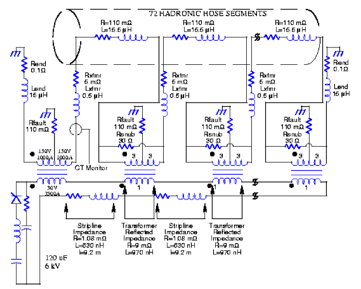
Figure 14: The electrical circuit simulated in Spice.[33] The 72 sections are connected to the transmission line through center-tapped transformers, with the transformers grounded to the decay pipe wall. A dummy impedence terminates the first and last transformer.

Because the decay volume is embedded in 2.5-3.0 m of concrete, it is necessary to have long leads from the power transmission line to the hadron hose feedthroughs. These leads consist of parallel flat copper sheets, and contribute an additional 2.5 $\mu$Henry inductance and 5 m$\Omega$ resistance in series with the hose segments.

7.2 Hose Circuit

Each hose segment is connected in parallel to a transmission line that runs down the side passageway of the decay tunnel. The transmission line is energized to 5000 V. The hose wire segments are connected through 73 3:1 transformers, with the upstream end of a hose segment center-tapped to the same transformer as the downstream end of the preceding hose segment. Dummy impedance loads are connected to the first and last transformers (see Figure 14). Current tranformers around the hose wire leads on the hose side of the transformer are used to monitor the current through each hose section and check for wire shorts or breaks.

The center-tapping of the transformers accomplishes three objectives. First, the voltage of any wire relative to the grounded vacuum decay pipe is cut by a factor of two, reducing the risk of voltage breakdown. Second, all the hose segments are effectively in series and receive the same currents to within 1 A according to simulations. Third, if a hose segment should fail and sever during operation, all the current is bypassed through the transmission line to the next hose segment.

7.3 Transmission Line

Because of the ambient conditions of the decay tunnel passage, we designed a coaxial transmission line made of 2 inch and 3 inch outer diameter concentric tubes of commercially available copper tubing. The center hot conductor is spaced from the outer return by circular standoffs spaced every meter along the transmission line. The standoffs are made of Peek plastic. With this design, no protection from ambient water or humidity is necessary. Measurements made on several prototype segments indicate that commercially available copper tubing (schedule ’K’) has a resistance of 1.6 m$\Omega$ per 9 m length and the concentric tubes have an inductance 900 $\mu$H. We also found that poor-quality weld joints can dominate the resistance of each 9 m transmission line segment. A schematic drawing of the transmission line design is shown in Figure 15.

Figure 15: Schematic drawing of the coaxial transmission line in the decay tunnel. Concentric 3” and 2” outer diameter Copper tubing are spaced from one another by Peek insulating rings. Connections between the center transmission line conductor and the transformers are accomplished by welding 3” Copper tubing “Tee’s” to the end of each outer conductor segment, and a 2” “elbow” to the end of each inner conductor segment.

.

7.4 Circuit Simulation

We have simulated the hadron hose circuit using Spice, including the inductance and resistance of the hose wire segments, penetration leads through the concrete, and transmission line. Furthermore, the Spice model included variations in the series resistance between hose wire segments due to the different temperatures of the hose wires at different positions along the beamline. A schematic of the simulated circuit is shown in Figure 14.

Figure 16: Spice simulation of the current and voltage pulse on a hadron hose wire segment. Indicated are the input voltage $V_{\mbox{input}}$ on each wire segment, the voltage difference $\Delta V$ between upstream and downstream end of the wire, and the currents for the hottest and the coolest of the wire segments in the beamline.

The results of the simulation,shown in Figure 16, have 3 important features. First, the variation of the delivered current during the beam spill is 1 Amp, or 0.1 %. Second, the voltage of the input ($V_{\mbox{input}}$ in Figure 16) is no more than 150 V anywhere, and the voltage difference between input and output ends ($\Delta V$ in Figure 16) is no more than 250 V. This means that the most challenging location for voltage breakdown is restricted to the 20 cm gap between hose wire segments. Third, while the temperatures of the hose segments in the decay volume vary from 80^∘ C at the downstream end to 150^∘ C near the upstream end of the decay tunnel (see Section 11), it is seen that the segments’ currents vary by less than 1 Amp.

8 Voltage Breakdown

The hose wire will have a voltage drop across each segment of 250 Volts. This voltage inside the 0.1 - 1.0 Torr vacuum of the NuMI decay pipe poses two potential problems. First, if the potential drop is too large then electrical breakdown could occur between the hose segments, which are separated by $\sim$ 20 cm. As shown in Figure 17, the Paschen curve [34] reaches a minimum of 400 Volts in the pressure range of 0.1 - 1.0 Torr relevant for the NuMI decay volume. Limiting the voltage drops inside the decay volume to 250 V provides a margin of safety against voltage breakdown.

Figure 17: Breakdown voltage of a hose wire segment inside a 6” diameter vacuum chamber as a function of the vacuum chamber pressure.

The second problem is the ionization of gas in the decay pipe from charged particles in the beam. This residual gas ionization could result in an electrical breakdown or in a current deposited on the wire which modifies the expected current pulse. Assuming the particle flux through the decay pipe is $6~{}\times~{}10^{13}$ particles/spill, an energy deposition of $dE/dx_{min}=1.82$ MeV/(g/cm²) in air, and scaling for the 0.17-1.7 mg/l density of air at the 0.1-1.0 Torr decay pipe pressure, the potential current collected on a 9 m hose wire segment is in the range between 9 to 90 Amp, ignoring effects of ion mobilities, recombination, etc.

We measured the ion current collected on a hose wire segment from ionized residual gas in a beam test at the Fermilab Booster Accelerator. An 8 GeV proton beam was passed through a vacuum chamber with 75 $\mu$m thick Ti entrance and exit windows. Inside the vacuum chamber, segments of hose wire segments were placed at spacings of 20 cm and 10 cm apart from one another, representing the distance between hose segments in NuMI before and after 10 years’ worth of creep. The beam passed directly between two wires, so that ionization between the wires would drift to the two electrodes, one at voltage and the other at ground. The data presented here were taken at 4.4$\times 10^{12}$ particles per 1.56 $\mu$sec spill, with $\sim 10$% variation between spills. The beam spot size was approximately 1 cm RMS, as measured by profile chambers which were retracted for most of the run. The ionization current was measured using a Pearson model 4100 current readout toroid around the high voltage leads to the chamber and read out in a digitizing scope.

Figure 18: Oscilloscope traces of two beam spills passing through the hose bell jar. The potential difference between the wires and the pressure inside the bell jar are indicated.

Figure 19: Total charge collected on the hose wire during the beam spill (left plot) and integrating for 25$\mu$sec after the beam spill (right plot) at several wire voltages and chamber pressures.

Figure 18 shows two typical events at different vacuum chamber pressures from the beam test taken at 400 V potential difference between the 10 cm-separated wires. The 1.56 $\mu$sec beam spill occurs between 1.75-3.25 $\mu$sec. The sign of the current is positive for electron flow back to the power supply from the hose wire, consistent with what would be expected for electron current flow from the gas to a positive voltage wire and ion current flowing to the grounded wire. In Figure 19, the total charge is integrated over the 1.56 $\mu$sec spill time and over the 25 $\mu$sec oscilloscope sweep time for each event. Data at several potential differences and pressures was recorded. It is perhaps interesting to note that the 200 V data shows no particular accentuated behaviour at moderate pressures, while an increasingly large charge is collected at moderate pressure for larger voltages. This effect perhaps indicates the onset of electrical breakdown consistent with the Paschen curve.

The data from Figure 19 may also be compared to the naive calculation of expected ionization current in air. Using the same numbers as above and the 66 cm path length of the beam through the vacuum chamber, we would expect 0.42 $\mu$Coulomb of charge released in the residual gas at 100 mTorr. This estimate agrees roughly with our data for 500 V, but is invalid at higher pressures or lower voltages, indicating that recombination effects are important. Furthermore, only 10% of the collected charge arrives during the beam spill time (evidently the drift time is long). Extrapolating this data to the NuMI beam conditions, the current deposited on the hose wire during the NuMI beam spill will be 0.02-0.2 Amps, which is well below the pulsed current of 1000 Amps.

9 Wire Creep

At temperatures of order 1/3 the melting point, many materials under strain experience plastic flow, or ’creep’. The melting point of pure aluminum is 640^∘C, suggesting that creep is a concern for the hose wire at temperatures near 200^∘C. The effect of creep can be detrimental to the hadron hose for two reasons: (1) it can lead to the failure of a hose wire segment which cannot be replaced after the beam has run; (2) the hose wire segments could break down electrically to adjacent segments if creep causes the wires to stretch too close to neighboring wires. We have performed two measurements of creep of anodized Aluminum alloy 1350 wires and determined a maximum desirable operating temperature of 150^∘C.

Figure 20: Summary of creep data for Aluminum 1350. The upper 3 plot symbols refer to wires with 10 $\mu$m anodization thickness and were taken with the 1 m ovens over a period of a year. The lower two refer to data from the 13 m oven with wires of with 10 $\mu$m or 17 $\mu$m thick anodization layer. The horizontal line at 2.5 mm/m/year indicates the requirement that the hose sections not be permitted to be closer than 10 cm after 10 years of NuMI operation.

The two measurements of Al creep rates were performed by heating aluminum wires under tension. The wires were heated by placing them inside concentric steel tubes which were separated by high temperature plastic. The inner tube was wrapped in heating tape, and the outer wrapped in fiberglass insulation. Thermocouples monitored the interior chambers. Wires suspended inside the tube were fixed at one end and at the other protruded outside the oven to a brass weight which kept the wire under tension. Dial indicators tracked the location of the weights over time. The first setup consisted of 1 m long ovens which were operated for 1 year. The second setup was a 13 m oven containing 30 wires and operated for one month. In the small ovens, anodized wire with 10 $\mu$m thick Aluminum oxide coating was tested. In the large oven, wires with both 10 $\mu$m and 17 $\mu$m thick anodization layers were tested. The large oven was used as well to straighten segments of hose wire for installation in the NuMI beamline, by annealing out the coil from the spool.

Figures 20 shows the data collected from all the 1 m tubes. In the small oven, large creep rates were measurable for temperatures greater than 180^∘C, the data below this temperature were consistent with zero creep. Better sensitivity was achieved with the large oven, in which a creep rate of 1.8$\times 10^{-4}$/year was observed with the 17-$\mu$m thick coatings at 290PSI = 4 MPa tension at 145^∘C. The thicker anodization appeared to have a factor of 5 or more smaller creep rate than the 10$\mu$m anodization.

10 Hose Thermal Measurements

Heat dissipates from the hose wire mainly by blackbody radiation and by conduction through the residual decay pipe atmosphere to the outer decay pipe wall. We performed measurements of heat dissipation from the hose wire via both of these mechanisms. These measurements serve as inputs to a detailed thermal model of the hose wire during beam operation.

Figure 21: Schematic diagram of the vacuum chamber used to measure the emissivity of coated wires and study the effect of gas cooling. A wire is suspended under tension and heated under a known current. The heated wire’s elongation is measured via a survey marker on the wire. TC’s 1-8 are thermocouples.

The thermal measurements of hose wire heat dissipation are performed using a vacuum chamber (see Figure 21) in which a known current is passed through a hose wire segment suspended under tension at its central axis. The inside walls of the vacuum chamber are lined with black plastic. The controlled $i^{2}r$ power input is balanced by blackbody radiation to the walls, by conduction through the wire to its ends, and (possibly) by conduction through the chamber gas to the walls. The wire comes to equilibrium at a temperature which is monitored by its elongation. Viewports to the vacuum chamber allow monitoring of the elongation through an optical telescope.

To interpret the experimental data on wire elongation, a thermal model of the vacuum chamber and the wire is developed. The temperature rise of the wire in a small time interval $\Delta t$ is

$$\Delta T=\frac{1}{mC_{p}}(P_{in}-P_{out}^{rad}-P_{out}^{gas}-P_{out}^{cond})\Delta t,$$ (4)

where $P_{out}^{rad}$ is the blackbody radiated power, $P_{out}^{gas}$ is the power conducted through the chamber gas (=0 at sufficiently low pressures), $P_{out}^{cond}$ is power conducted through the wire material to the ends, $m$ is the wire mass, and $C_{p}$ is its heat capacity.

The input power to the wire $P_{in}=i^{2}\rho l/A_{wire}$, where $i$ is the applied current, $l=580$ cm is the length and $A_{wire}=0.042$ cm² is the wire cross sectional area, and $\rho=2.96~{}\mu\Omega$-cm is our measured value of the resistivity of Al1350 at 20^∘C. The resistivity slope is $0.010~{}\mu\Omega$-cm/^∘C. We used our measured value for the coefficient of thermal expansion of the anodized wire, $2.25\times 10^{-5}$.

Figure 22: Observed elongation of the 580 cm long wire vs time with $4.5\times 10^{-6}$ Torr pressure in the vacuum chamber. The current was switched on at $t=0$ min and switched off at $t=90$ min. The curves are from the thermal model. The current on the wire is 15 Amps (left) and 7.5 Amps (right).

The blackbody power radiated is described by

$$P_{out}^{rad}=\sigma_{B}A_{wire}F_{12}(T_{wire}^{4}-T_{wall}^{4}),$$ (5)

where $\sigma_{B}$ is the Stefan-Boltzmann constant, $A_{wire}=2\pi r\Delta l$ is the surface area, $T_{wire}$ ($T_{wall}$) is the temperature of the wire (vacuum chamber wall). The factor $F_{12}$ is given by

$$\frac{1}{F_{12}}=\frac{1}{\varepsilon_{wire}}+\frac{A_{wire}}{A_{wall}}(\frac{1}{\varepsilon_{wall}}-1),$$ (6)

where $\varepsilon_{wire}$ is the wire emissivity to be measured in this study, $A_{wall}$ is the surface area of the vacuum chamber walls, and $\varepsilon_{wall}$ is the wall emissivity. Because $A_{wire}/A_{wall}\sim 0.01$, we placed a black polyethelene liner inside the vacuum chamber to keep $F_{12}\approx\varepsilon_{wire}$ to within $\sim~{}0.5$%. The plastic liner caused imperfect thermal contact of the walls with the room, so that $T_{wall}$ was not simply room temperature. $T_{wall}$ was measured using thermocouples placed inside the vacuum chamber and on the wire ends (see Figure 21).

Four measurements were made with $i~{}=~{}7.5,10,15,$ and 20 Amps, yielding emissivity values of $\varepsilon~{}=~{}$0.61, 0.59, 0.60, and 0.61, respectively. The results of the measurements with $i~{}=~{}15$ and 7.5 Amps are shown in Figure 22. The systematic uncertainties on this measurement include a $\pm 0.01$ uncertainty from the 1% measurement uncertainty in the coefficient of thermal expansion and a $\pm 0.01$ uncertainty from the 1% measurement uncertainty in the electrical resistivity. The simulation indicates that the thermal conductivity and heat capacity uncertainties lead to negligible uncertainty on $\varepsilon_{wire}$. We quote $\varepsilon_{wire}~{}=~{}0.61~{}\pm~{}0.03$ for the wire tested with 17$\mu$m anodization layer.

Figure 23: Observed elongation of the 580 cm long wire for several vacuum chamber pressures and three different wire currents.

The same chamber was used to measure the effect of gas cooling. Figure 23 shows several measurements of wire elongation at different currents and vacuum chamber pressures. Apparently gas cooling is important above $10^{-5}$ Torr, and the term $P_{out}^{gas}$ in Equation 4 must be included. We assume a form of

$$P_{out}^{gas}=\frac{2\pi k}{ln(r_{wall}/r_{wire})}\Delta l(T_{wire}-T_{wall}),$$ (7)

where $\Delta l$ is the length of an element of the wire into which the wire is divided, and $k$ is the heat conduction coefficient of air, which is 0.024 W/cm/^oC at atmospheric pressure. We use the data in Figure 23 to derive $k$ as a function of pressure, setting $\varepsilon_{wire}~{}=~{}0.61$. This is shown in Figure 24. The rise of our apparent value for $k$ above 0.0239 W/cm/^∘C at 10 Torr may indicate that convection is additionally important as the pressure increases. These values for $k$ are used to simulate the cooling of the hose in the NuMI decay pipe.

Figure 24: Derived values for the gas heat conduction coefficient versus pressure from the data of Figure 23.

11 Hose Wire Thermal Modelling

During operation of the beam, the energy deposited in the Hadron Hose wire comes from $i^{2}r$ heating and from particle interactions in the hose wire. The hose wire dissipates heat primarily through blackbody radiation and cooling from the residual gas in the decay volume. Measurements of these two effects were presented in the previous section. Cooling via conduction to the wire ends also occurs, but to only small effect. In this section we calculate the final equilibrium temperature of the wire during beam operation. Assuming a 150^∘C upper limit for the operating temperature temperature of the wire to limit the effects of long-term creep, we calculate the maximum current pulse length acceptable to be 0.6 ms.

Figure 25: The energy deposited along the hose wire due to ionizing particles in the beam as calculated using the MARS Monte Carlo [25]. The calculation is performed both for the case of no current in the hose and with the magnetic field of the hose turned on. The peak at zero is due to protons striking a 2 m unpulsed section of wire placed in front of the pulsed sections..

In one pulse, the current deposits a heat load of $\Delta Q=\int i(t)^{2}rdt$ delivered to the wire, which grows linearly with the pulse duration. For an RMS current duration of 310 (620) $\mu$sec, the simulation of the hadron hose circuit indicates that $\int i(t)^{2}dt=215$ (430) Amp²-sec. At room temperature, this value for the energy deposited would correspond to 18 (36) J deposited in one 9 m long hose segment per beam spill, corresponding to 1 (2) Watt/meter.

Figure 26: Calculation of the hose wire temperature from a thermal model of the hose wire in the NuMI beam as a function of distance along the wire from the beginning of the decay volume. (left) Calculation for a fixed current pulse length of 600$\mu$sec half-width, several values of wire emissivity $\varepsilon=$0.4, 0.5 0.6, 0.7, and 0.8. (right) Calculation for $\varepsilon=0.7$ and current pulse lengths of 400, 600, and 800 $\mu$sec.

Energy deposition in the hose wire is dominated by interactions of primary protons that did not interact in the target. These protons enter the decay pipe with a mean scattering angle of 0.25 mrad with respect to the nominal beam direction. These protons are focused by the hose field directly into the wire. Because the protons leave the target travelling radially, all unreacted protons are eventually focused into the wire. An analytical calculation of the distance at which protons strike the hose wire [32] yields an energy deposition of 3.5 Watt/meter inside the first 30 m of hose wire.

We confirmed this calculation using the MARS beamline Monte Carlo package [25]. This simulation includes the NuMI target, focusing horns, and all material upstream of the hose such as the target shielding and vacuum decay pipe window. Thus, the simulation includes energy deposited in the wire from protons as well as by any other showering particles that are created in secondary interactions upstream in the beamline. The result of this simulation, shown as a function of position along the hose wire, is shown in Figure 25. The peak at zero meters arises from protons travelling along the beam axis which interact in the 2 m unpulsed section of the hose, while the energy deposited downstream results from protons which multiple scatter in the target and are brought back to the beam axis by the hose field. Not suprisingly, the simulation indicates that with the hose field turned off, this second component disappears. The additional deposited energy compared to the analytic calculation indicates the magnitude of energy deposition from showering particles created in upstream material in the beamline.

The expectation for the hose wire temperature in the NuMI beam is calculated using the thermal model of Section 10, with the addition of the beam heating and of gas cooling. The beam heating term is taken from Figure 25. The temperature of the NuMI decay pipe wall at $r_{wall}=100$ cm is set to $T_{wall}=55^{\circ}$C, based on a MARS simulation of the energy deposited in the decay pipe. We assume a value of the heat transfer coefficient of $k=0.0239$W/cm/^∘C at 0.1-1.0 Torr from Figure 24. Thermal conduction is allowed to the end of each 9 m hose segment, which are also constrained to 55^∘C. In the calculation, each hose segment is subdivided into three parts: a central 9 m segment which receives both $i^{2}r$ and beam heating, and two 1 m ’leads’ which bring the hose current in from the decay pipe walls to the center of the pipe which receive only $i^{2}r$ heating (no beam heating).

The results of the calculation are shown in Figure 26. In the figure, the basic shape of the temperature distribution follows the beam energy deposition calculated in Figure 25, as may be expected. Based on this calculation of wire heating, a pulse length of 600 $\mu$sec is acceptable, assuming a wire emissivity $\varepsilon\sim 0.6-0.7$ as achieved for 17$\mu$m anodization.

12 Radiological Issues

The NuMI beam produces large numbers of hadrons, neutrons, gammas, and other particles which can cause activation of the surrounding earth and rock. This activation affects underground aquifers in the vicinity of the beamline. The NuMI decay volume and the target hall are shielded from the surrounding rock by poured concrete or stacked steel blocks, respectively. The thickness of target hall steel is $\sim$ 2 m and the decay volume concrete shield ranges from 3 m at the upstream end to 2 m at the downstream end. In addition a hadron beam stop, consisting of a $2\times 2$ m² by 3 m longitudinal depth Aluminum core surrounded by a 2 m thick layer of stacked steel blocks, is located at the end of the decay volume

We studied whether the hose could increase the radioactivation of the surrounding earth. Such an increase could result, in principle, from interactions of the remnant proton beam with the hose wire. These interactions occur along the full length of the decay pipe, including the most downstream sections where the shielding is thinnest. Without the hose, much of this component of the beam power is absorbed in the hadron stop.

We used the MARS beamline Monte Carlo [25] to simulate any increase in activation of the surrounding rock resulting from such proton interactions in the wire. All particles above 100 MeV were tracked in the simulation, except neutrons, for which the threshold was 10 MeV. The radioactivation measure is the density of ’stars’ in the surrounding rock per proton on target. A star is a nuclear interaction above 50 MeV in the rock caused by particles from the beam. The density of stars is tabulated in Table 2, and is averaged over the 1 m layer of rock surrounding the shielding. For reference, NuMI will deliver $4\times 10^{20}$ protons on target per year. According to the simulation, operation of the Hadron Hose does increase the star densities in different regions around the NuMI beamline. These results indicate that the shielding planned for the NuMI beam line can accomodate inclusion of the Hadron Hose without modification.

Region	No Hose	Hose
Target Hall	0.59 $\pm$ 0.01	0.49 $\pm$ 0.06
DV Upstream	4.4 $\pm$ 0.4	6.3 $\pm$ 0.4
DV Middle	2.1 $\pm$ 0.2	2.4 $\pm$ 0.1
DV Downstream	1.0 $\pm$ 0.1	0.9 $\pm$ 0.1

Table 2: Densities ($\times 10^{-11}$) of ’stars’ (nuclear interactions above 50 MeV) per cm³ of rock per proton on target in the NuMI low-energy beam. The star densities are tabulated for the rock surrounding the target hall and for three longitudinal segments of rock around the decay volume.

13 Conclusions

We have investigated the potential impact of a new focusing system, the Hadron Hose, for conventional neutrino beams. This system was developed for the NuMI beam at Fermilab, and may be of benefit to future conventional ’super beams’ because of its increase in neutrino event yield and ability to control systematic uncertainties due to particle production in the target or imperfections in the rest of the neutrino beam elements.

14 Acknowledgements

We thank our NuMI and MINOS colleagues, particularly Karol Lang, Doug Michael, and Stan Wojcicki, for discussions and encouragement. We thank Ron Dimelfi, John Hall, Nikolai Mokhov, Howie Pfeffer, Steve Sansone, and Sergei Striganov for helpful consultations. We acknowledge the valuable contributions of the University of Texas Physics Department mechanical support shops, the Fermilab Particle Physics, Beams, Survey/Alignment, and Mechanical Support Divisions, and in particular Virgil Bocean, Cary Kendziora, Stephen Pordes, Bob Webber, and James Lackey. This work was supported by the U.S. Department of Energy, DE-AC02-76CH3000, DE-FG03-93ER40757 and DE-FG02-91ER40654, the National Science Foundation, NSF/PHY-0089116, and the Fondren Foundation.

References

- [1] S. van der Meer, CERN Yellow Report CERN-61-07 (1961).
- [2] G. Danby et al., Phys. Rev. Lett. 9, 36 (1962).
- [3] G.Bernardini et al., Proc. Int’l Conf. on Elementary Particles, Sienna, vol. 1 (1963) 523; M. Giesch et al., Proc. Int’l Conf. on Elementary Particles, Sienna, vol. 1 (1963) 536; C. Angelini et al. (BEBC Collaboration), Phys. Lett. B179, 307 (1986); F. Bergsma et al. (CHARM Collaboration), Phys. Lett. B142, 103 (1984); F. Dydak et al. (CDHS Collaboration), Phys. Lett. B134, 281 (1984).
- [4] G. Acquistapace et al., The West Area Neutrino Facility, CERN-ECP/95-14 (1995); P. Astier et al. (Nomad Collaboration), Nucl. Phys. B611, 3 (2001); A.G. Cocco et al. (Chorus Collaboration), Proc. XXXVI Recontres de Moriond (2001).
- [5] L. Ahrens et al. (BNL E734), Phys. Rev. D31, 2732 (1985); B. Blumenfeld et al. (BNL E776), Phys. Rev. Lett. 19, 2237 (1989).
- [6] S.H. Ahn et al. (K2K Collaboration), Phys. Lett. B511, 178 (2001).
- [7] G.N. Taylor, et al. (FNAL E338 Collaboration), Phys. Rev. D28, 2705 (1983).
- [8] E.B. Brucker, et al. (FNAL E564 Collaboration), Phys. Rev. D34, 2183 (1986); I.E. Stockdale, et al. (CCFR Collaboration), Phys. Rev. Lett. 52, 1384 (1985); N. Ushida, et al. (FNAL E531 Collaboration), Phys. Rev. Lett. 57, 2897 (1986).
- [9] N.I. Stepa, Motion of a Relativistic Charged Particle in the Magnetic Field Produced by a Constant Cylindrical Current of a Rarefied Plasma, Soviet Phyics – Techn. Physics 4, 1237 (1960).
- [10] Die Bewegung Geladener Teilchen im Magnetfeld eines Geraden Stromdurch-flossenen Drahten, Zeit. f. Naterf. 14A, 47 (1959).
- [11] S. van der Meer, The Beam Guide, CERN-62-16, April 17, 1962.
- [12] E. Regenstreif, Contributions to the Theory of the Beam Guide, CERN 64-41, September 24, 1964.
- [13] Y. Itow et al., “The JHF-Kamioka Neutrino Project”, Letter of Intent, KEK Report 2001-4, ICRR Report 477-2001-7, TRIUMF Report TRI-PP-01-05, June, 2001.
- [14] V. Barger et al., hep-ph/0103052 (FERMILAB-FN-703), Addendum to Report FN-692 to the Fermilab Directorate, March 5, 2001.
- [15] V. D. Barger, D. Marfatia and K. Whisnant, “Neutrino superbeam scenarios at the peak,” in Proc. of the APS/DPF/DPB Summer Study on the Future of Particle Physics (Snowmass 2001) ed. R. Davidson and C. Quigg, arXiv:hep-ph/0108090.
- [16] J. J. Gomez-Cadenas et al. [CERN working group on Super Beams Collaboration], “Physics potential of very intense conventional neutrino beams, arXiv:hep-ph/0105297.
- [17] J. Hylen et al. “Conceptual Design for the Technical Components of the Neutrino Beam for the Main Injector (NuMI),” Fermilab-TM-2018, Sept., 1997.
- [18] The MINOS Collaboration, “The MINOS Detectors Technical Design Report,” Fermilab NuMI-L-337, Oct. 1998, S. Wojcicki, spokesman.
- [19] G. Ambrosini et al. (SPY Collaboration), Phys. Lett. B420 (1998) 225; Phys. Lett. B425 (1998) 208; Eur. Phys. J. C10 (1999) 605.
- [20] H.W. Atherton et al., CERN 80:07, 1980.
- [21] D.S. Barton et al., Phys. Rev. D27, 2580 (1983)
- [22] A. Brenner et al., Phys. Rev. D26, 1497 (1982).
- [23] T. Eichten et al., Nucl. Phys. B44, 333 (1972).
- [24] M. Bonesini, A. Marchionni, F. Pietropaolo, and T. Tabarelli de Fatis, “On Particle Production for High Energy Neutrino Beams,” Eur. Phys. J. C20, 13-27 (2001).
- [25] N.V. Mokhov, “The MARS Monte Carlo”, Fermilab FN-628 (1995); O.E. Krivosheev et al., Proc. of the Third and Fourth Workshops on Simulating Accelerator Radiation Environments (SARE3 and SARE4), Fermilab-Conf-98/043(1998) and Fermilab-Conf-98/379(1998).
- [26] A.J. Malensek, “Empirical Formula for Thick Target Particle Production,” Fermilab FN-341, Oct. 1981.
- [27] GEANT Detector Description and Simulation Tool, CERN Program Library, W5013 (1994).
- [28] A. Ferrari and P.R. Sala, ’Fluka Monte Carlo,’ ATLAS Internal Note ATL-PHYS-97-113, Proc. of the Workshop on Nuclear Reaction Data and Nuclear Reactors Physics, Design and Safety, ICTP, Trieste, Italy 1996. Publ. by World Scientific, A.Gandini, G.Reffo, eds.
- [29] K. Simonyi, ”Theoretishe elektrotechnick” 1956, Veb Deutsher Verlag der Wissenschaften, Berlin.
- [30] D. Beavis et al., “Long Baseline Neutrino Oscillation Experiment, E889, Physics Design Report,” BNL-52459, April, 1995.
- [31] Metals Handbook, 9th Edition, Vol. 2, ASM Handbook Committee, American Society for Metals.
- [32] R.H. Milburn, “Theory of the Hadron Hose”, Fermilab Technical Memo NuMI-B-271 (1997).
- [33] L. Nagel, “SPICE2, A Computer Program to Simulate Semiconductor Circuits,” Memo-No. ERL-M520, University of California, Berkeley, May, 1975; D. O. Pederson, “A Historical Review of Circuit Simulation,” IEEE Transactions on Circuits and Systems, vol. CAS-31, No. 1, January 1984; T. Quarles, A. R. Newton, D. O. Pederson, A. Sangiovanni-Vincentelli, “SPICE 3B1 User’s Guide,” University of California, Berkeley, April, 1987.
- [34] E. Kuffeland and M. Abdullah, “High Voltage Engineering”, 1970, Pergamon Press.
- [35] ICRU Report 31 “Average Energy Required to Produce An Ion Pair” (International Commission on Radiation Units and Measurements, 1 May, 1979).