Determination of the $\bar{B}\rightarrow D^{*}\ell\bar{\nu}$ Decay Width and $|V_{cb}|$

Abstract

In the Standard Model, the charged current of the weak interaction is governed by a unitary quark mixing matrix that also leads to $CP$ violation. Measurement of the Cabibbo-Kobayashi-Maskawa (CKM) matrix elements is essential to searches for new physics, either through the structure of the CKM matrix, or a departure from unitarity. We determine the CKM matrix element $|V_{cb}|$ using a sample of $3\times 10^{6}$ $B\bar{B}$ events in the CLEO detector at the Cornell Electron Storage Ring. We determine the yield of reconstructed $\bar{B^{0}}\to D^{*+}\ell\bar{\nu}$ and $B^{-}\to D^{*0}\ell\bar{\nu}$ decays as a function of $w$, the boost of the $D^{*}$ in the $B$ rest frame, and from this we obtain the differential decay rate $d\Gamma/dw$. By extrapolating $d\Gamma/dw$ to $w=1$, the kinematic end point at which the $D^{*}$ is at rest relative to the $B$, we extract the product $|V_{cb}|{\cal F}(1)$, where ${\cal F}(1)$ is the form factor at $w=1$. We find $|V_{cb}|{\cal F}(1)=0.0431\pm 0.0013{\text{(stat.)}}\pm 0.0018{\text{(syst.)}}$. We combine $|V_{cb}|{\cal F}(1)$ with theoretical results for ${\cal F}(1)$ to determine $|V_{cb}|=0.0469\pm 0.0014{\text{(stat.)}}\pm 0.0020{\text{(syst.)}}\pm 0.0018{\text{(theo.)}}$. We also integrate the differential decay rate over $w$ to obtain ${\cal B}(\bar{B^{0}}\to D^{*+}\ell\bar{\nu})=(6.09\pm 0.19\pm 0.40)\%$ and ${\cal B}(B^{-}\to D^{*0}\ell\bar{\nu})=(6.50\pm 0.20\pm 0.43)\%$.

I Introduction

The elements of the Cabibbo-Kobayashi-Maskawa (CKM) quark mixing matrix Ckm ; cKM are fundamental parameters of the Standard Model and must be determined experimentally. Measurement of the matrix elements tests unified theories that predict the values of these elements. It also offers a means of searching for physics beyond the Standard Model by testing for apparent deviations of the matrix from unitarity, deviations that could arise if new physics affected the measurement of one of its elements. The status of this test is often displayed using the famous “Unitarity Triangle”unitaritytriangle . The CKM matrix element $|V_{cb}|$ sets the length of the base of this triangle, and it scales the constraint imposed by $\epsilon_{K}$ (This constraint scales as $|V_{cb}|^{4}$), the parameter that quantifies $CP$ violation in the mixing of neutral kaons K0cpv .

Two strategies are available for precise measurement of $|V_{cb}|$, both of which rely on the underlying quark decay $b\to c\ell\bar{\nu}$, where $\ell$ indicates $e^{-}$ or $\mu^{-}$. The first method combines measurements of the inclusive semileptonic branching fraction and lifetime to determine the semileptonic decay rate of the $B$ meson, which is proportional to $|V_{cb}|^{2}$. Theoretical quark-level calculations give the proportionality constant, thereby determining $|V_{cb}|$, with some uncertainties from hadronic effects. This first approach relies on the validity of quark-hadron duality, the assumption that this inclusive sum is insensitive to the details of the various final states that contribute.

The second approach uses the specific decay mode $\bar{B}\to D^{*}\ell\bar{\nu}$ or $\bar{B}\to D\ell\bar{\nu}$. The rate for these decays depends not only on $|V_{cb}|$ and well-known weak decay physics, but also on strong interaction effects, which are parameterized by form factors. In general, these effects are notoriously difficult to quantify, but because the $b$ and $c$ quark are both massive compared to the scale of hadronic physics, $\bar{\Lambda}\approx 0.5$ GeV, heavy-quark symmetry relations can be applied to $\bar{B}\to D^{(*)}\ell\bar{\nu}$ decays hqs_voloshin ; hqs_isgur ; hqs_luke ; hqs_falk ; hqs_neubert . In the limit $m_{b},m_{c}\to\infty$, the form factor is unity at zero recoil, the kinematic point at which the final state $D^{(*)}$ is a rest with respect to the initial $B$ meson. Corrections to the infinite-mass limit are then calculated using an expansion in powers of $\bar{\Lambda}/m_{Q}$. Luke showed hqs_luke that the first-order correction vanishes for pseudoscalar-to-vector transitions, making $D^{*}\ell\bar{\nu}$ decays more attractive theoretically than $D\ell\bar{\nu}$ for $|V_{cb}|$ determination. Heavy Quark Effective Theory (HQET) hqet_grinstein ; hqet_eichten ; hqet_georgi ; hqet_koerner ; hqet_mannel exploits the heavy-quark symmetry and offers a rigorous framework for quantifying the hadronic effects with relatively small uncertainty dslnu_neubert ; dslnu_falk .

In this paper, we report more fully on a recently published letter measurement of $|V_{cb}|$ using $\bar{B}\to D^{*}\ell\bar{\nu}$ decays that are detected in the CLEO II detector at the Cornell Electron Storage Ring (CESR). The $\bar{B}\to D^{*}\ell\bar{\nu}$ decays are fully reconstructed, apart from the neutrino. The analysis takes advantage of the kinematic constraints available at the $\Upsilon(4S)$ resonance, where the data were collected, to suppress backgrounds, help distinguish $D^{*}\ell\bar{\nu}$ from similar modes such as $D_{1}\ell\bar{\nu}$, and provide superb resolution on the decay kinematics. This analysis is the first since a previous CLEO result oldcleo to use not only $\bar{B}^{0}\to D^{*+}\ell\bar{\nu}$ decays, but also $B^{-}\to D^{*0}\ell\bar{\nu}$ decays blvthesis . Consistency between these two modes is a valuable cross-check of our results.

We reconstruct $D^{*+}$ candidates and their charge conjugates (charge conjugates are implied throughout this paper) through the modes $D^{*+}\to D^{0}\pi^{+}$ and $D^{0}\to K^{-}\pi^{+}$, and we reconstruct $D^{*0}$ candidates through the modes $D^{*0}\to D^{0}\pi^{0}$, $D^{0}\to K^{-}\pi^{+}$, and $\pi^{0}\to\gamma\gamma$. Each $D^{*}$ candidate is combined with an electron or muon candidate. We then divide the reconstructed candidates into bins of $w$, where $w$ is the scalar product of the $B$ and $D^{*}$ four-velocities, and equals the relativistic $\gamma$ of the $D^{*}$ in the $B$ rest frame. Given these yields as a function of $w$, we fit simultaneously for parameters describing the form factor ${\cal F}(w)$ and the normalization at $w=1$. This normalization is proportional to the product $|V_{cb}|^{2}{\cal F}^{2}(1)$, and combined with the theoretical results for ${\cal F}(1)$, it gives us $|V_{cb}|$.

II Event Samples

Our analysis uses $3.33\times 10^{6}$ $B\bar{B}$ events (3.1 ${\text{fb}^{-1}}$) produced on the $\Upsilon(4S)$ resonance at the Cornell Electron Storage Ring (CESR) and detected in the CLEO II detector. In addition, the analysis uses a sample of 1.6 ${\text{fb}^{-1}}$ of data collected slightly below the $\Upsilon(4S)$ resonance for the purpose of subtracting continuum backgrounds. Because of miscalibration of low-energy showers in the calorimeter in a subset of the data, we use only $3.04\times 10^{6}$ $B\bar{B}$ events (2.9 ${\text{fb}^{-1}}$) produced on the $\Upsilon(4S)$ resonance and 1.5 ${\text{fb}^{-1}}$ of data collected below the $\Upsilon(4S)$ resonance for reconstructing $B^{-}\to D^{*0}\ell\bar{\nu}$ candidates.

The CLEO II detector cleonim has three central tracking chambers, immersed in a 1.5 T magnetic field, that measure charged particle trajectories and momenta. The momentum resolution is 5 MeV$/c$ (12 MeV$/c$) for particles with a momentum of 1 GeV$/c$ (2 GeV$/c$) (typical for the lepton and the $K$ and $\pi$ from the $D^{0}$) and 3 MeV$/c$ for particles with momentum less than 250 MeV$/c$ (typical for the $\pi^{+}$ from the $D^{*+}$). A CsI(Tl) calorimeter surrounds both the tracking chambers and a time-of-flight system that is not used for this analysis. The calorimeter provides photon detection and assists with electron identification. The energy resolution of the calorimeter is 3.8 MeV for 100 MeV photons, a typical energy for photons from the decay of the $\pi^{0}$ from the $D^{*0}$ decay. The outermost detector component consists of plastic streamer counters layered between iron plates and provides detection of muons.

We also use simulated event samples from a Geant-based geant Monte Carlo simulation. With this Monte Carlo, we produce large samples of simulated $\bar{B}\to D^{*}\ell\bar{\nu}$ decays as well as a sample of $16\times 10^{6}$ $B\bar{B}$ events to study some backgrounds.

III Event Reconstruction

The $\Upsilon(4S)$ is produced and decays at rest, and each daughter $B$ meson is produced with a momentum of about 0.3 GeV$/c$. As a result, $\Upsilon(4S)\to B\bar{B}$ events tend to be isotropic, or “spherical,” with particles carrying energy in all directions. When the electron-positron collisions in CESR do not produce $\Upsilon(4S)$’s, they can produce, among other things, $q{\bar{q}}$ quark pairs, where the $q$ is a $c$, $s$, $u$, or $d$ quark. Because the mass of these quark pairs is much lower than the energy of the beam, the daughter particles of these quarks’ hadronization have higher momenta than the $B$’s. These events tend to have a more “jetty” appearance; that is, the energy in the event tends to be distributed back-to-back. The ratio of Fox-Wolfram moments $H_{2}/H_{0}$ r2 measures an event’s jettiness, with values of the ratio approaching zero for spherical events, and approaching one for jetty events. To suppress non-$B\bar{B}$ events, we require that the ratio of Fox-Wolfram moments $H_{2}/H_{0}$ be less than 0.4, a condition satisfied by 98% of $B{\bar{B}}$ events containing a $D^{*}\ell\bar{\nu}$ decay.

To reconstruct $D^{*}\ell\bar{\nu}$ candidates we first form $D^{0}\to K^{-}\pi^{+}$ candidates from all possible pairs of oppositely charged tracks, alternately assigning one the kaon mass and the other the pion mass. We require a fiducial cut of $|\cos\theta|\leq 0.9$ for tracks, where $\theta$ is the polar angle of the track’s momentum vector with respect to the $e^{+}e^{-}$ beam axis. Tracks outside this fiducial region are excluded from consideration because they are poorly measured, having passed through the endplate of one of the inner tracking chambers and therefore either traversing a significant amount of material before entering the outer tracking chamber or never entering it at all. We reconstruct the invariant mass $m(K\pi)$ of the $D$ candidate with a resolution of about 7 MeV$/c^{2}$, accepting candidates that lie in the window $|m(K\pi)-1.865|\leq 0.020$ GeV$/c^{2}$. The $m(K\pi)$ distributions for $D^{*+}\ell\bar{\nu}$ and $D^{*0}\ell\bar{\nu}$ candidates are shown in Fig. 1.

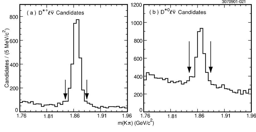
Figure 1: The $m(K\pi)$ distribution for (a) $D^{*+}\ell\bar{\nu}$ and (b) $D^{*0}\ell\bar{\nu}$ candidates. All requirements are met except $|m(K\pi)-1.865|\leq 0.020$ GeV$/c^{2}$. We accept candidates that fall between the arrows.

The pions produced in the decay $D^{*}\to D\pi$ have low momentum ($<250$ MeV$/c$) because the combined mass of the $D^{0}$ and $\pi$ is within 8 MeV$/c^{2}$ of the mass of the $D^{*}$. We label these pions “slow.” For $D^{*+}$ candidates, we add a slow $\pi^{+}$ candidate to a $D^{0}$ candidate, requiring that the slow pion have the same charge as the pion from the $D$ decay. This pion must also satisfy $|\cos\theta|\leq 0.9$. The $K$ and $\pi$ are fit to a common vertex, and then the slow $\pi^{+}$ and $D^{0}$ are fit to a second vertex using the beam spot constraint. For this vertexing we use error matrices from our Kalman fitter Kalman . We then form $\Delta m\equiv m(K\pi\pi)-m(K\pi)$. We look at $\Delta m$ rather than $m(K\pi\pi)$ because subtracting the $D^{0}$ candidate mass from the $D^{*}$ candidate mass cancels some errors in reconstructing the $D^{0}$. A plot of $\Delta m$ for $D^{*+}$ candidates is shown in Fig. 2(a). The vertex constraints improve the resolution by about 20% to 0.7 MeV$/c^{2}$. We require $|\Delta m-0.14544|\leq 0.002$ GeV$/c^{2}$ for $D^{*+}$ candidates.

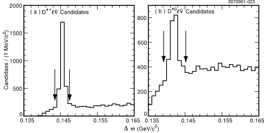
Figure 2: The $\Delta m$ distribution for (a) $D^{*+}\ell\bar{\nu}$ and (b) $D^{*0}\ell\bar{\nu}$ candidates. All requirements are met except $|\Delta m-0.14544|\leq 0.002$ GeV$/c^{2}$ for $D^{*+}\ell\bar{\nu}$ and $|\Delta m-0.1422|\leq 0.003$ GeV$/c^{2}$ for $D^{*0}\ell\bar{\nu}$. We accept candidates that fall between the arrows.

For $D^{*0}$ candidates, we add a slow $\pi^{0}\to\gamma\gamma$ candidate to the $D^{0}$ candidate. We construct $m(\gamma\gamma)$ for slow $\pi^{0}$ candidates from showers in the CsI calorimeter whose position is inconsistent with extrapolation of any of the tracks reconstructed in the event. We require that the lateral pattern of energy deposition in the calorimeter be consistent with expectations for a photon. Particles with $|\cos\theta|>0.71$ travel through the endplate of the outermost tracking chamber before reaching the calorimeter, again traversing a significant amount of material. We therefore require that both photon candidates satisfy $|\cos\theta|\leq 0.71$ so as to remain in the part of the calorimeter with the best energy and position resolution. Both photons must have energy greater than 30 MeV to limit background from soft showers. We also require the invariant mass $m(\gamma\gamma)$ to give the known $\pi^{0}$ mass within roughly three times the resolution of 5 MeV$/c^{2}$: $0.120$ GeV$/c^{2}$ $\leq m(\gamma\gamma)\leq 0.150$ GeV$/c^{2}$. The $\Delta m$ resolution for $D^{*0}$’s is about 0.9 MeV$/c^{2}$, so we require $|\Delta m-0.1422|\leq 0.003$ GeV$/c^{2}$. The $\Delta m$ distribution for $D^{*0}$ candidates is shown in Fig. 2(b), and the $m(\gamma\gamma)$ distribution is shown in Fig. 3.

Figure 3: The $m(\gamma\gamma)$ distribution for $D^{*0}\ell\bar{\nu}$ candidates. All requirements are met except $0.120$ GeV$/c^{2}$ $\leq m(\gamma\gamma)\leq 0.150$ GeV$/c^{2}$. We accept candidates that fall between the arrows.

Finally, we require the momentum of the $D^{*}$ candidate to be less than $\frac{1}{2}\sqrt{E_{B}^{2}-m(K\pi\pi)^{2}}$, (approximately 2.5 GeV$/c$), where $E_{B}$ is the energy of the beam. This requirement suppresses background from non-$B\bar{B}$ events.

We next combine the $D^{*}$ candidate with a lepton candidate, accepting both electrons and muons. Electrons are identified using the ratio of their energy deposition in the CsI calorimeter to the reconstructed track momentum, the shape of the shower in the calorimeter, and their specific ionization in the tracking chamber. We require our candidates to lie in the momentum range $0.8$ GeV$/c$ $\leq p_{e}<2.4$ GeV$/c$, where the upper bound is the end point of $D^{*}\ell\bar{\nu}$ decays. This momentum selection is approximately 93% efficient for ${\bar{B}}\to D^{*}e^{-}{\bar{\nu}}$ decays. We require muon candidates to penetrate two layers of steel in the solenoid return yoke, or about 5 interaction lengths. Only muons with momenta above about 1.4 GeV$/c$ satisfy this requirement; we therefore demand that muon candidates lie in the momentum range $1.4$ GeV$/c$ $\leq p_{e}<2.4$ GeV$/c$. This more restrictive muon momentum requirement has an efficiency of approximately 61%. We require both muon and electron candidates to be in the central region of the detector ($|\cos\theta|\leq 0.71$), where efficiencies and hadron misidentification rates are well understood. The charge of the lepton must match the charge of the kaon, and in the case of $D^{*+}\ell\bar{\nu}$ decays, be opposite that of the slow pion.

The remaining reconstruction relies on the kinematics of the $\bar{B}\to D^{*}\ell\bar{\nu}$ decay. We first reconstruct $\cos\theta_{B-D^{*}\ell}$, the angle between the $D^{*}$-lepton combination and the $B$ meson, computed assuming that the only unreconstructed particle is a neutrino. This variable helps distinguish $\bar{B}\to D^{*}\ell\bar{\nu}$ decays from background and is necessary for the reconstruction of $w$. To form $\cos\theta_{B-D^{*}\ell}$, we first note that the 4-momenta of the particles involved in $\bar{B}\to D^{*}\ell\bar{\nu}$ decay are related by

$$p_{\nu}^{2}=(p_{B}-p_{D^{*}}-p_{\ell})^{2}.$$ (1)

Setting the neutrino mass to zero gives

$$0=m_{B}^{2}+m(D^{*}\ell)^{2}-2\left[E(B)E(D^{*}\ell)-{\mathbf{p}}(B)\cdot{\mathbf{p}}(D^{*}\ell)\right].$$ (2)

We solve for the only unknown quantity, the angle between the $B$ meson and the $D^{*}$-lepton pair:

$$\cos\theta_{B-D^{*}\ell}=\frac{2E(B)E(D^{*}\ell)-m_{B}^{2}-m(D^{*}\ell)^{2}}{2|{\mathbf{p}}(B)||{\mathbf{p}}(D^{*}\ell)|}.$$ (3)

In forming $\cos\theta_{B-D^{*}\ell}$, we use the momenta of the $D^{*}$ and lepton candidates as well as the $B$ mass ershov and average $B$ momentum, measured in our data. At CESR, a symmetric $e^{+}e^{-}$ collider operating on the $\Upsilon(4S)$ resonance, the $B$ energy and therefore momentum is given by the energy of the colliding beams. Instead of relying on beam energy measurements based on storage ring parameters and subject to significant uncertainties, we determine the average $B$ momentum directly using fully reconstructed $B$ decays to hadrons. The energy spread of the beams and run-to-run energy variations lead to a distribution of $B$ energies and momenta. By measuring the momentum distribution of fully reconstructed hadronic $B$ decays in our data sample, we determine the energy spread intrinsic to CESR, which is then used to simulate $B\bar{B}$ pair production in our Monte Carlo. For $\cos\theta_{B-D^{*}\ell}$ we use the true $D^{*}$ mass rather than the reconstructed $m(K\pi\pi)$ to avoid a bias in the $\cos\theta_{B-D^{*}\ell}$ distribution of the $\Delta m$ sideband, which we use to determine a background.

We next estimate $w$ for each candidate. Exact reconstruction of $w$, the boost of the $D^{*}$ in the rest frame of the $B$, requires knowledge of the $B$ momentum vector. Although the magnitude of the $B$ momentum is known, the $B$ direction is unknown. However, it must lie on a cone with opening angle $\theta_{B-D^{*}\ell}$ around the $D^{*}\ell$ direction. We calculate $w$ for all $B$ flight directions on this cone and average the smallest and largest values to estimate $w$, with typical resolution of 0.03. We divide our sample into ten equal bins from 1.0 to 1.5, where the upper bound is just below the kinematic limit of 1.504. For a few candidates, the reconstructed $w$ falls outside our range; we assign these to the first or last bin as appropriate. Figure 4 shows the distributions of reconstructed $w$ minus generated $w$ in the third and ninth $w$ bins for simulated $\bar{B^{0}}\to D^{*+}\ell\bar{\nu}$ and $B^{-}\to D^{*0}\ell\bar{\nu}$ decays.

In the high $w$ bins, we suppress background with minor loss of signal efficiency by restricting the cosine of the angle between the momenta of the $D^{*}$ and of the lepton ($\cos\theta_{D^{*}-\ell}$). The distribution of $\cos\theta_{D^{*}-\ell}$ versus $w$ is shown in Fig. 5 for simulated $\bar{B}\to D^{*}\ell\bar{\nu}$ decays. Some backgrounds are uniformly distributed in this angle. The accepted angles are listed in Table 1.

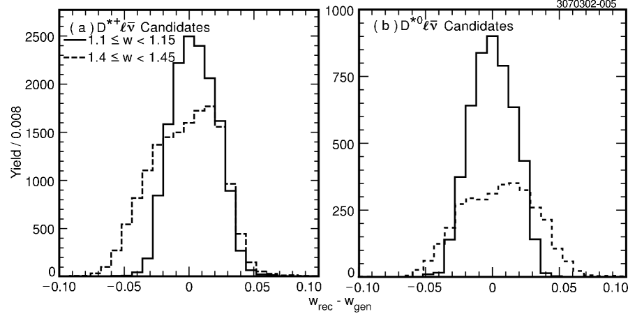
Figure 4: The difference between the reconstructed $w$ and generated $w$ for simulated $D^{*+}\ell\bar{\nu}$ (a) and $D^{*0}\ell\bar{\nu}$ (b) decays in the intervals $1.1\leq w<1.15$ (solid) and $1.4\leq w<1.45$ (dashed). The normalization of all four histograms is arbitrary.

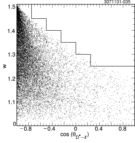
Figure 5: The distribution of $w$ versus $\cos\theta_{D^{*}-\ell}$ for simulated $D^{*}\ell\bar{\nu}$ decays with lepton momentum between 0.8 GeV$/c$ $\leq p_{\ell}<$ 2.4 GeV$/c$. We accept candidates that fall below and to the left of the stair-step line.

Table 1: The accepted regions of the cosine of the angle between the $D^{*}$ and the lepton in each $w$ bin.

$w$ bin	$w$ limits	Accepted $\cos\theta_{D^{*}-\ell}$
		min.	max.
1-5	$<1.25$	$-1.00$	$1.00$
6	1.25-1.30	$-1.00$	$0.25$
7	1.30-1.35	$-1.00$	$0.00$
8	1.35-1.40	$-1.00$	$-0.25$
9	1.40-1.45	$-1.00$	$-0.50$
10	$\geq 1.45$	$-1.00$	$-0.75$

IV Extracting the $D^{*}\ell\bar{\nu}$ Yields

IV.1 Method

At this stage, our sample of candidates contains not only $\bar{B}\to D^{*}\ell\bar{\nu}$ decays, but also $\bar{B}\to D^{**}\ell\bar{\nu}$ and $\bar{B}\to D^{*}\pi\ell\bar{\nu}$ decays and various backgrounds. In the following, we refer to $\bar{B}\to D^{**}\ell\bar{\nu}$ and non-resonant $\bar{B}\to D^{*}\pi\ell\bar{\nu}$ decays collectively as $\bar{B}\to D^{*}X\ell\bar{\nu}$ decays. In order to disentangle the $D^{*}\ell\bar{\nu}$ from the $D^{*}X\ell\bar{\nu}$ decays, we use a binned maximum likelihood fit likelihood to the $\cos\theta_{B-D^{*}\ell}$ distribution. As shown in Fig. 6, $\bar{B}\to D^{*}\ell\bar{\nu}$ decays are concentrated in the physical region, $-1\leq\cos\theta_{B-D^{*}\ell}\leq 1$, while the missing mass of the $D^{*}X\ell\bar{\nu}$ decays allows them to populate $\cos\theta_{B-D^{*}\ell}<-1$. In this fit, the normalizations of the various background distributions are fixed and we allow the normalizations of the $D^{*}\ell\bar{\nu}$ and the $D^{*}X\ell\bar{\nu}$ components to float. For each $w$ bin, we fit over a $\cos\theta_{B-D^{*}\ell}$ region chosen to include 95% of the $D^{*}X\ell\bar{\nu}$ events in that bin. These regions are listed in Table 2.

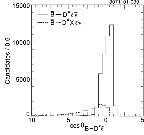
Figure 6: The $\cos\theta_{B-D^{*}\ell}$ distributions for simulated $D^{*}\ell\bar{\nu}$ and $D^{*}X\ell\bar{\nu}$ decays.

Table 2: The regions of $\cos\theta_{B-D^{*}\ell}$ over which we perform a binned maximum likelihood fit.

$w$ bin	$w$ limits	$\cos\theta_{B-D^{*}\ell}$ fit region
		min.	max.
1-6	$<1.30$	$-8.0$	$1.5$
7	1.30-1.35	$-6.0$	$1.5$
8	1.35-1.40	$-4.0$	$1.5$
9	1.40-1.45	$-3.0$	$1.5$
10	$\geq 1.45$	$-2.0$	$1.5$

The distributions of the $D^{*}\ell\bar{\nu}$ and $D^{*}X\ell\bar{\nu}$ decays come from Monte Carlo simulation. We simulate $D^{*}\ell\bar{\nu}$ decays using the form factor of caprini and include the effect of final-state radiation ($\bar{B}\to D^{*}\ell\bar{\nu}\gamma$) using Photos photos . For $D^{*}X\ell\bar{\nu}$, we model $D^{**}\ell\bar{\nu}$ modes according to ISGW2 isgw2 and non-resonant $D^{*}\pi\ell\bar{\nu}$ from Goity and Roberts goityroberts . Our model for $D^{*}X\ell\bar{\nu}$ is dominated by approximately equal parts of $D_{1}\ell\bar{\nu}$ and $D^{*}\pi\ell\bar{\nu}$. The other backgrounds, and how we obtain their $\cos\theta_{B-D^{*}\ell}$ distributions and normalizations, are described in the next section.

IV.2 Backgrounds

There are several sources of decays other than $\bar{B}\to D^{*}\ell\bar{\nu}$ and $\bar{B}\to D^{*}X\ell\bar{\nu}$. We divide these backgrounds into five classes: continuum, combinatoric, uncorrelated, correlated, and fake lepton. As an indication of the relative importance of the various backgrounds, in Table 3 we give both the fraction ${B_{i}}/{N_{\text{tot}}}$ of candidates from each background source relative to all candidates and the ratio $B_{i}/S$ of each background source to $D^{*}\ell\bar{\nu}$ signal. Because signal events populate the physical region $-1\leq\cos\theta_{B-D^{*}\ell}\leq 1$, we compute both ${B_{i}}/{N_{\text{tot}}}$ and $B_{i}/S$ using only candidates in this “signal region.” We discuss each background and how we determine it below.

Table 3: The contribution of each background $B_{i}$ to the total number of candidates $N_{\text{tot}}$ in the range $-1\leq\cos\theta_{B-D^{*}\ell}\leq 1$ for the $D^{*+}\ell\bar{\nu}$ and $D^{*0}\ell\bar{\nu}$ analyses. The relative size to $D^{*}\ell\bar{\nu}$ signal $B_{i}/S$ is also given for the same $\cos\theta_{B-D^{*}\ell}$ interval.

Background	$D^{*+}\ell\bar{\nu}$ Contribution		$D^{*0}\ell\bar{\nu}$ Contribution
	${B_{i}}/{N_{\text{tot}}}$ (%)	$B_{i}/S$ (%)	${B_{i}}/{N_{\text{tot}}}$ (%)	$B_{i}/S$ (%)
Continuum	$3.8$	$4.7$	$2.8$	$5.1$
Combinatoric	$7.9$	$10$	$38$	$70$
Uncorrelated	$4.4$	$5.6$	$4.7$	$8.6$
Correlated	$0.4$	$0.5$	$0.1$	$0.2$
Fake Lepton	$0.5$	$0.6$	$0.2$	$0.4$

IV.2.1 Continuum background

At the $\Upsilon(4S)$ we detect not only resonance events ($\Upsilon(4S)\to B\bar{B}$), but also non-resonant events such as $e^{+}e^{-}\to q\bar{q}$. This background contributes about 4% of the candidates within the signal region for $D^{*+}\ell\bar{\nu}$ decays, and about 3% for $D^{*0}\ell\bar{\nu}$ decays. This is about 5% relative to the $D^{*}\ell\bar{\nu}$ signal. In order to subtract background from this source, CESR runs one-third of the time slightly below the $\Upsilon(4S)$ resonance. For this continuum background, we use the $\cos\theta_{B-D^{*}\ell}$ distribution of candidates in the off-resonance data scaled by the ratio of luminosities and corrected for the small difference in the $e^{+}e^{-}\to q{\bar{q}}$ cross sections at the two center-of-mass energies. In reconstructing $\cos\theta_{B-D^{*}\ell}$, we scale the energy and momentum of the $D^{*}$ and lepton by the ratio of the center-of-mass energies and use the $B$ momentum measured in on-resonance data to compute the $B$ energy. This continuum background includes combinatoric and fake lepton backgrounds arising from continuum processes.

IV.2.2 Combinatoric background

Combinatoric background candidates are those in which one or more of the particles in the $D^{*}$ candidate does not come from a true $D^{*}$ decay. This background contributes 8% of the candidates in the signal region for $D^{*+}\ell\bar{\nu}$; for $D^{*0}\ell\bar{\nu}$, which suffers from random shower combinations and does not benefit from the charge correlation of the slow pion, this background contributes 38% of the candidates in the signal region. Relative to the $D^{*}\ell\bar{\nu}$ signal, the combinatoric background is 10% for $D^{*+}\ell\bar{\nu}$ and 70% for $D^{*0}\ell\bar{\nu}$.

The $\cos\theta_{B-D^{*}\ell}$ distribution of the combinatoric background is provided by $D^{*}$-lepton combinations in the high $\Delta m$ sideband. We choose the $\Delta m$ sidebands of $0.155$ GeV$/c^{2}$ $\leq\Delta m<0.165$ GeV$/c^{2}$ for $D^{*+}\ell\bar{\nu}$ and $0.147$ GeV$/c^{2}$ $\leq\Delta m<0.165$ GeV$/c^{2}$ for $D^{*0}\ell\bar{\nu}$. For values of $\Delta m$ above these ranges, the slow pions tend to be faster, and therefore $\cos\theta_{B-D^{*}\ell}$ tends to be larger, while regions closer to the $\Delta m$ signal region include signal decays in which the slow pion is poorly reconstructed. With this choice, only 3.5% and 0.4% of the $D^{*}\ell\bar{\nu}$ decays fall in the sideband for $D^{*+}\ell\bar{\nu}$ and $D^{*0}\ell\bar{\nu}$, respectively.

The normalization of the $\Delta m$ sideband candidates is determined in each $w$ bin from a fit to the $\Delta m$ distribution with the sum of properly reconstructed $D^{*}$’s and the combinatoric background. The line-shape for the $D^{*}$ peak is taken from simulated $D^{*}\ell\bar{\nu}$ decays. The $D^{*0}\ell\bar{\nu}$ line-shape includes $D^{*0}$ candidates in which only one of the two photons constituting the $\pi^{0}$ was correct. Since these candidates preferentially populate the $\Delta m$ signal region, a few (3.9% of all $D^{*0}\ell\bar{\nu}$ decays) remain after our combinatoric background subtraction and are included in our $D^{*0}\ell\bar{\nu}$ signal. For $D^{*+}\ell\bar{\nu}$ we assume a background shape of the form

$$n(\Delta m-m_{\pi})^{a}\exp\left\{\left[c_{1}(\Delta m-m_{\pi})+c_{2}(\Delta m-m_{\pi})^{2}\right]\right\},$$ (4)

where $c_{1}$ and $c_{2}$ are constants fixed using an inclusive $D^{*+}$ sample, and we vary $n$, $a$, and the normalization of the signal peak. For $D^{*0}\ell\bar{\nu}$ we assume a background shape of the form

$$n(\Delta m-m_{\pi})^{a}\exp\left[{b(\Delta m-m_{\pi})}\right]$$ (5)

and vary $n$, $a$, $b$, and the normalization of the signal peak. The fits for $D^{*+}\ell\bar{\nu}$ and $D^{*0}\ell\bar{\nu}$ are shown for a representative $w$ bin in Fig. 7. The normalizations are shown in Fig. 8.

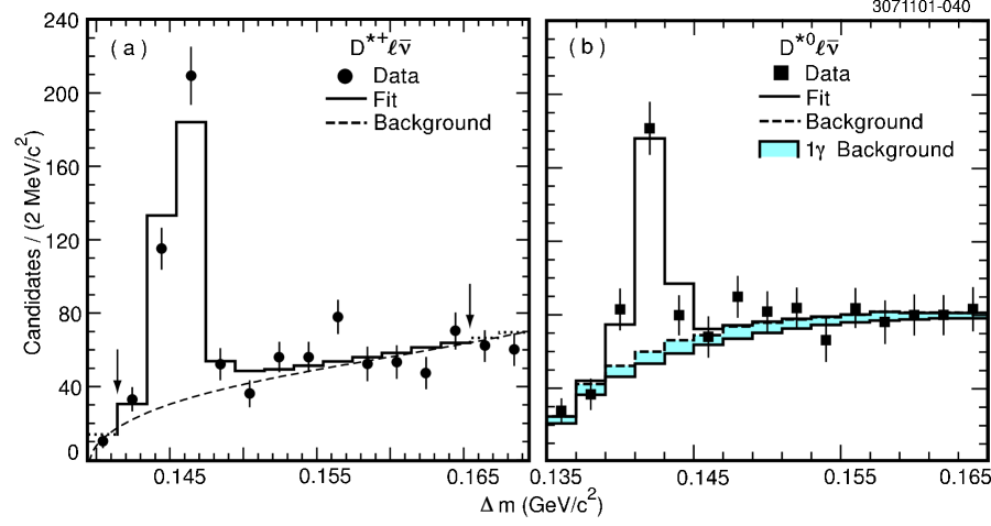
Figure 7: The $\Delta m$ distribution of candidates in the third $w$ bin ($1.1\leq w<1.15$) for (a) $D^{*+}\ell\bar{\nu}$ candidates and (b) $D^{*0}\ell\bar{\nu}$ candidates with the result of the fit superimposed. The data (solid circles or squares) are superimposed with the combinatoric background distribution (dashed curve) and the sum of the background and the $D^{*}$ signal (solid histogram). In (a) the arrows delimit the fit region. In (b), the shaded histogram shows combinations in which only one of the two photons forming the $\pi^{0}$ candidate was correct. Unless indicated otherwise, the error bars provided in all figures are statistical only.

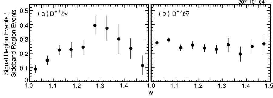
Figure 8: The ratio of the number of combinatoric background candidates in the $\Delta m$ signal region to the number in the $\Delta m$ sideband, as determined from fits to $\Delta m$ for (a) $D^{*+}\ell\bar{\nu}$ and (b) $D^{*0}\ell\bar{\nu}$. The $\cos\theta_{B-D^{*}\ell}$ distribution of the combinatoric background is provided by the sideband candidates normalized by this ratio.

As a test of this background estimate, we carry out the same procedure used in data on a sample of 16 million simulated $B\bar{B}$ events. Because combinatoric background originates from random combinations of tracks and showers, we expect our Monte Carlo, which is tuned to reproduce track and shower multiplicity and momentum distributions of $B$ decays, to provide a reliable check of the background estimation procedure. We compare the true background in the $\Delta m$ signal region with the background estimate formed using the $\Delta m$ sideband region. There is a concern that kinematic differences between candidates in the $\Delta m$ signal and sideband regions could cause a difference in the $\cos\theta_{B-D^{*}\ell}$ shape of the estimated and true backgrounds. Figures 9 and 10 show the true and estimated backgrounds for the Monte Carlo sample. We observe that the shapes do differ for $D^{*+}\ell\bar{\nu}$, consistent with the effect of the strong momentum dependence of the slow-pion efficiency (Section VI.2). The agreement is better for $D^{*0}\ell\bar{\nu}$. We evaluate the systematic error from this sideband technique in Section VI.1.2.

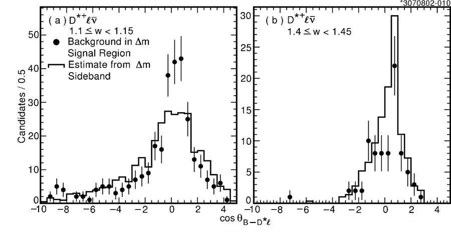
Figure 9: From Monte Carlo, the $\cos\theta_{B-D^{*}\ell}$ distribution for $D^{*+}\ell\bar{\nu}$ combinatoric background candidates in the $\Delta m$ signal region (points) and for scaled candidates from the $\Delta m$ sideband (histogram) for (a) $1.1\leq w<1.15$ and (b) $1.4\leq w<1.45$. The sideband events are normalized using a fit to the $\Delta m$ distribution as described in the text.

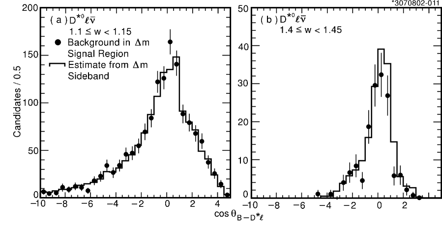
Figure 10: From Monte Carlo, the $\cos\theta_{B-D^{*}\ell}$ distribution for $D^{*0}\ell\bar{\nu}$ combinatoric background candidates in the $\Delta m$ signal region (points) and for scaled candidates from the $\Delta m$ sideband (histogram) for (a) $1.1\leq w<1.15$ and (b) $1.4\leq w<1.45$. The sideband events are normalized using a fit to the $\Delta m$ distribution as described in the text.

This method of background estimation overlooks a small component of the combinatoric background, a component that arises from $D^{*}$ decays in which the slow pion is properly found but the $D^{0}$ candidate is constructed from the products of a $D^{0}$ decay other than $D^{0}\to K^{-}\pi^{+}$. Although the $D^{0}$ is misreconstructed, this background will still peak in the $\Delta m$ signal region. Most of these candidates have $m(K\pi)$ below our signal region, but Monte Carlo simulation shows that $D^{0}\to\rho^{+}\pi^{-}/\rho^{-}\pi^{+}$ decays could contribute a few candidates to the $m(K\pi)$ and $\Delta m$ signal regions. Although these decay modes have not yet been observed, a combined branching fraction of 1.3% is plausible given the measured branching fraction of all $D^{0}\to\pi^{+}\pi^{-}\pi^{0}$ decays; with this branching fraction, these modes would increase our $D^{*}\ell\bar{\nu}$ yield by $(0.3\pm 0.2)\%$. In a sample of 16 million simulated $B\bar{B}$ decays, several other modes also contribute, bringing the total contribution to $(0.5\pm 0.3)\%$. The contributing modes are listed in Table 4. As this contribution has little effect on our results, and as the branching fractions of the main contributing modes ($D^{0}\to\rho^{+}\pi^{-}$ and $D^{0}\to\rho^{-}\pi^{+}$) are unmeasured, we account for it in the combinatoric background systematic error, but otherwise neglect it.

Table 4: Decay modes of the $D$, other than $D^{0}\to K^{-}\pi^{+}$, that are not fully subtracted by the $\Delta m$ sideband. The third column shows the expected contribution (relative to $D^{0}\to K^{-}\pi^{+}$) to the $D^{*}\ell\bar{\nu}$ yield from each mode in the $m(K\pi)$ and $\Delta m$ signal regions.

Mode	Branching Fraction(%)	Contribution(%)
$D^{0}\to K^{+}K^{-}$	$0.425\pm 0.016$	$0.05\pm 0.03$
$D^{0}\to\pi^{+}\pi^{-}$	$0.152\pm 0.009$	$0.02\pm 0.02$
$D^{0}\to K^{-}\bar{\ell}\nu$	$3.47\pm 0.17$	$0.02\pm 0.02$
$D^{0}\to\pi^{+}\pi^{-}\pi^{0}$	$1.6\pm 1.1$	$0.33\pm 0.24$
$D^{0}\to K^{-}\rho^{+}$	$10.8\pm 1.0$	$0.02\pm 0.02$
$D^{0}\to K^{*-}\pi^{+}$	$1.7\pm 0.2$	$0.01\pm 0.01$
$D^{0}\to\pi^{-}\bar{\ell}\nu$	$0.37\pm 0.06$	$0.07\pm 0.05$
Total		$0.52\pm 0.25$

IV.2.3 Uncorrelated background

Uncorrelated background arises when the $D^{*}$ and lepton come from the decays of different $B$ mesons in the same event. This background accounts for approximately 5% of the candidates in the signal region for both $D^{*+}\ell\bar{\nu}$ and $D^{*0}\ell\bar{\nu}$ decays, contributing 6% and 9% relative to $D^{*+}\ell\bar{\nu}$ and $D^{*0}\ell\bar{\nu}$, respectively. We obtain the $\cos\theta_{B-D^{*}\ell}$ distribution of this background by simulating each of the various sources of uncorrelated $D^{*}$’s and leptons and normalizing each one based on rates measured from or constrained by the data. We classify the $D^{*}$ and the lepton according to their respective sources because different sources give different momentum spectra for the $D^{*}$ and lepton, and therefore different distributions in $\cos\theta_{B-D^{*}\ell}$.

There are three components of uncorrelated background that contribute to both the $D^{*+}\ell\bar{\nu}$ and $D^{*0}\ell\bar{\nu}$ modes. The first component consists of a lower-vertex $D^{*}$ (i.e., from $b\to c$ transitions) combined with a secondary lepton (i.e., from $b\to c\to s\bar{\ell}\nu$) (primary leptons from the other $B$ have the wrong charge correlation); this is the largest component for the $D^{*+}\ell\bar{\nu}$ mode. Secondly, uncorrelated background can also occur when the $B^{0}$ and $\bar{B}^{0}$ mix or when a $\bar{D^{*}}$ from the upper-vertex (i.e., from $b\to\bar{c}$, as in $b\to c\bar{c}s$) is combined with a primary lepton (i.e., from $b\to c(u)\ell\bar{\nu}$). Finally, in the $D^{*0}\ell\bar{\nu}$ case, the largest source of uncorrelated background consists of candidates in which the $K$ and $\pi$ from a lower-vertex $D^{*}$ have been exchanged and paired with a primary lepton from the other $B$. (This background does not occur for $D^{*+}\ell\bar{\nu}$ because we constrain the charge of the slow-pion candidate to be opposite to that of the kaon.)

Table 5: The rate per $B\bar{B}$ pair used to normalize the $D^{*}$ elements of the uncorrelated background. The errors indicate the variation used to assess the systematic uncertainty in the background.

Rate	$p_{D^{*}}\leq 1.3$ GeV$/c$	$p_{D^{*}}>1.3$ GeV$/c$
lower-vertex, $D^{*+}$	0.281$\pm$0.032	0.242$\pm$0.015
lower-vertex, $D^{*0}$	0.231$\pm$0.031	0.272$\pm$0.014
upper-vertex, $D^{*+}$	0.048$\pm$0.024	0.012$\pm$0.006
upper-vertex, $D^{*0}$	0.048$\pm$0.024	0.004$\pm$0.002

We first determine the production rate of upper-vertex $D^{*}$’s from $B$ decays using the measured branching fractions of modes such as $\bar{B}\to D^{(*)}\bar{D}^{(*)}\bar{K}^{(*)}$DDK . We do this in two $D^{*}$ momentum bins, relying on our simulation of such decays for the $D^{*}$ momentum distribution. To determine the lower-vertex $D^{*}$ production rate, we measure the rate of inclusive $D^{*}$ production from $B$ decays in the data in each momentum bin and subtract the upper-vertex contribution from each. The results are shown in Table 5. We determine the background contribution from $D$’s reconstructed with exchanged $K$’s and $\pi$’s by studying inclusive $D^{*+}$ decays with the charge correlation of the slow pion reversed.

We normalize the primary lepton decay rate for leptons with momenta between 0.8 GeV$/c$ and 2.4 GeV$/c$ to its measured value of $(8.99\pm 0.42)$% roywang , where the error includes statistical and systematic errors; since this measurement was made at CLEO, we include only the systematic errors that are uncorrelated with our analysis. Likewise, we adjust the secondary lepton rate for leptons with momenta between 0.8 GeV$/c$ and 2.4 GeV$/c$ to its measured value of $(1.53\pm 0.12)$% roywang . Finally, we adjust $\chi_{d}$, the $B^{0}-\bar{B}^{0}$ mixing probability, to its measured value of $0.174\pm 0.009$ pdg .

IV.2.4 Correlated background

Correlated background candidates are those in which the $D^{*}$ and lepton are decay products of the same $B$, but the decay was not $\bar{B}\to D^{*}\ell\bar{\nu}$ or $\bar{B}\to D^{*}X\ell\bar{\nu}$. The most common sources are $\bar{B}\to D^{*}\tau^{-}\bar{\nu}$ followed by leptonic $\tau$ decay, and $\bar{B}\to D^{*}D_{s}^{(*)-}$ followed by semileptonic decay of the $D_{s}^{-}$. The uncorrelated background contributes 0.5% and 0.2% compared to the $D^{*+}\ell\bar{\nu}$ and $D^{*0}\ell\bar{\nu}$ signals, respectively. The background is small; we therefore rely on our Monte Carlo simulation to quantify it. The decay modes and branching fractions used are listed in Table 6.

Table 6: Modes that contribute to the correlated background, their assumed branching fractions (BF), and fraction of the total correlated background. The numbers given are for the $D^{*0}\ell\bar{\nu}$ mode. The contributions to the $D^{*+}\ell\bar{\nu}$ mode are similar.

Mode	BF pdg    (%)	Fraction(%)
$\bar{B}\to D^{*0}X\tau^{-}\bar{\nu}$	$1.65$	$36.0$
$\bar{B}\to D_{s}^{*-}D^{*0}$	$3.08$	$18.7$
$\bar{B}\to D^{*0}D^{(*)}K^{(*)}$	$5.6$	$18.7$
$\bar{B}\to D^{*0}\bar{D^{*}}$	$3.4$	$15.1$
$\bar{B}\to D_{s}^{-}D^{*0}$	$1.39$	$6.5$
$\bar{B}\to D^{*0}\gamma X$; $\gamma\to e^{+}e^{-}$	—	$3.6$
$\bar{B}\to D^{*0}\pi^{-}$; $\pi^{-}\to\mu^{-}\bar{\nu}$	$0.47$	$1.4$

IV.2.5 Fake lepton background

Fake lepton background arises when a hadron is misidentified as a lepton and is then used in our reconstruction. Fake leptons make up 0.5% of candidates in the signal region for $D^{*+}\ell\bar{\nu}$ and 0.2% for $D^{*0}\ell\bar{\nu}$; relative to signal, the background contributions are about 0.5%. To assess this background we repeat the analysis, using hadrons in place of the lepton candidates. After subtracting continuum and combinatoric backgrounds, we normalize the $\cos\theta_{B-D^{*}\ell}$ distributions with the probability for a hadron to fake an electron or muon. We measure the momentum-dependent fake probability using kinematically identified samples of hadrons: pions are identified using $K_{S}^{0}\rightarrow\pi^{+}\pi^{-}$ decays, kaons using $D^{*+}\rightarrow D^{0}\pi^{+}\rightarrow K^{-}\pi^{+}\pi^{+}$, and protons from $\Lambda\rightarrow p\pi^{-}$. The fake probabilities are then weighted by species abundance in $B$ decays and the momentum spectrum of hadronic tracks in events with an identified $D^{*+}$ to obtain an average fake rate of 0.035% for a hadronic track to fake an electron and 0.68% to fake a muon.

IV.2.6 $D^{*}\ell\bar{\nu}$ and $D^{*}X\ell\bar{\nu}$ $\cos\theta_{B-D^{*}\ell}$ distributions

The $\cos\theta_{B-D^{*}\ell}$ distributions of $D^{*}\ell\bar{\nu}$ and $D^{*}X\ell\bar{\nu}$ decays are obtained from simulated $B\bar{B}$ events in which one of the $B$’s is required to decay to $D^{*}\ell\bar{\nu}$ or $D^{*}X\ell\bar{\nu}$. Since the other $B$ in the event also decays, the $\cos\theta_{B-D^{*}\ell}$ distributions can contain the same backgrounds listed above. Using generator-level information, we veto all background sources except the combinatoric background, for which we perform the same $\Delta m$ sideband subtraction used in the data. In the sideband subtraction, we use the signal-region to sideband ratios obtained from $\Delta m$ fits for the data. (Comparison of these ratios for data and simulated $B\bar{B}$ decays shows them to be compatible.) This sideband subtraction correctly accounts for the small number of signal decays that populate the $\Delta m$ sideband.

IV.3 $\bar{B}\to D^{*}\ell\bar{\nu}$ yields

Having obtained the distributions in $\cos\theta_{B-D^{*}\ell}$ of the signal and background components, we fit for the yield of $D^{*}\ell\bar{\nu}$ candidates in each $w$ bin. Two representative fits are shown for $D^{*+}\ell\bar{\nu}$ in Fig. 11 and $D^{*0}\ell\bar{\nu}$ in Fig. 12. The quality of the fits is good, as is agreement between the data and fit distributions outside the fitting region. We summarize the observed $D^{*}\ell\bar{\nu}$ and $D^{*}X\ell\bar{\nu}$ yields in Fig. 13.

The $D^{*}X\ell\bar{\nu}$ yields correspond to branching fractions of ${\cal B}(\bar{B}\to D^{*+}X\ell\bar{\nu})=(0.97\pm 0.24\text{(stat.)})$% and ${\cal B}(\bar{B}\to D^{*0}X\ell\bar{\nu})=(0.32\pm 0.55\text{(stat.)})$%. These are somewhat lower than past measurements alephdstx ; delphidstx , but because the analysis is not optimized for these modes the systematic uncertainties on these branching fractions are large, of order $\pm 30\%$ for $D^{*+}$ and $\pm 60\%$ for $D^{*0}$, dominated by model dependence in the efficiency to satisfy our lepton momentum criteria, uncertainty in the correlated and uncorrelated backgrounds, and radiative effects in $D^{*}\ell\bar{\nu}$.

Figure 11: The $\cos\theta_{B-D^{*}\ell}$ distribution (solid circles) for $D^{*+}\ell\bar{\nu}$ in the intervals (a) $1.1\leq w<1.15$ and (b) $1.4\leq w<1.45$ with the results of the fit superimposed (histogram). The arrows indicate the fit ranges.

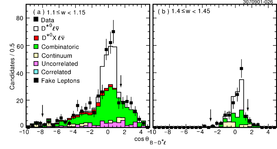
Figure 12: The $\cos\theta_{B-D^{*}\ell}$ distribution (solid squares) for $D^{*0}\ell\bar{\nu}$ in the intervals (a) $1.1\leq w<1.15$ and (b) $1.4\leq w<1.45$ with the results of the fit superimposed (histogram). The arrows indicate the fit ranges.

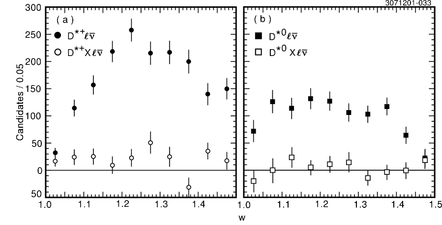
Figure 13: The observed (a) $D^{*+}\ell\bar{\nu}$ and $D^{*+}X\ell\bar{\nu}$ yields and (b) $D^{*0}\ell\bar{\nu}$ and $D^{*0}X\ell\bar{\nu}$ yields in each $w$ bin.

In order to test the quality of our $\cos\theta_{B-D^{*}\ell}$ fits and the modeling of the signal and backgrounds, we compare the observed $D^{*}$ energy and lepton momentum spectra with expectations for candidates in the signal-rich region $\left\lvert\cos\theta_{B-D^{*}\ell}\right\rvert\leq 1$. The $\cos\theta_{B-D^{*}\ell}$ fits provide the normalizations of the $D^{*}\ell\bar{\nu}$ and $D^{*}X\ell\bar{\nu}$ components. Figure 14 shows the $D^{*}$ energy distributions, and Figs. 15 and 16 show the electron and muon momentum spectra, repsectively, for $D^{*+}\ell\bar{\nu}$ and $D^{*0}\ell\bar{\nu}$ candidates. We find good agreement between the data and our expectations.

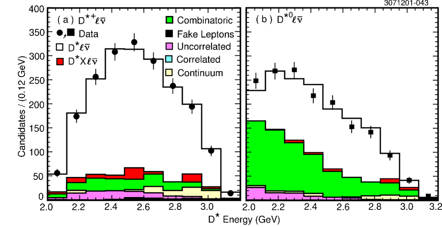
Figure 14: The $D^{*}$ energy distribution of (a) $D^{*+}\ell\bar{\nu}$ candidates and (b) $D^{*0}\ell\bar{\nu}$ candidates in the region $\left\lvert\cos\theta_{B-D^{*}\ell}\right\rvert\leq 1$ for all $w$ bins combined.

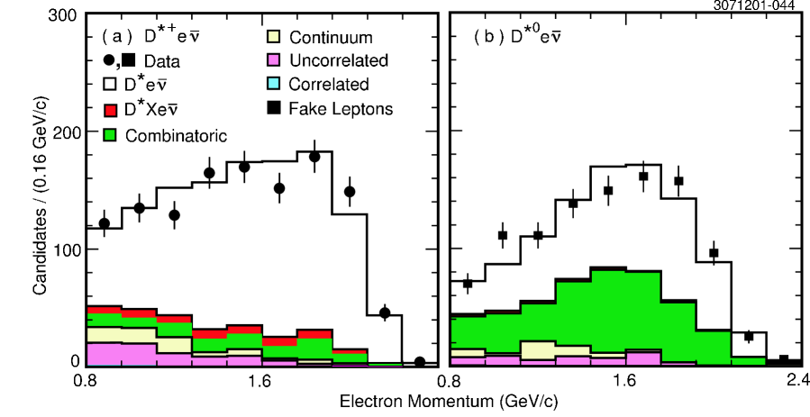
Figure 15: The electron momentum spectrum for (a) $D^{*+}e^{-}\bar{\nu}$ candidates and (b) $D^{*0}e^{-}\bar{\nu}$ candidates in the region $\left\lvert\cos\theta_{B-D^{*}\ell}\right\rvert\leq 1$ for all $w$ bins combined.

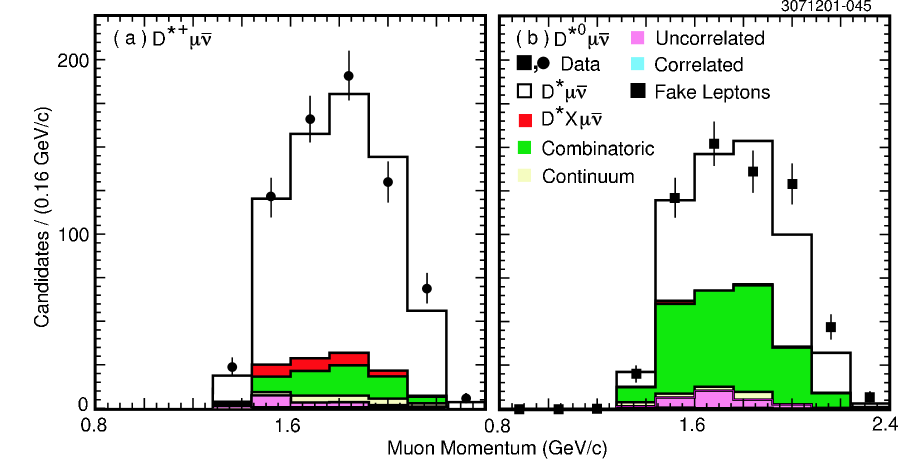
Figure 16: The muon momentum spectrum for (a) $D^{*+}\mu^{-}\bar{\nu}$ candidates and (b) $D^{*0}\mu^{-}\bar{\nu}$ candidates in the region $\left\lvert\cos\theta_{B-D^{*}\ell}\right\rvert\leq 1$ for all $w$ bins combined.

V The $|V_{cb}|$ Fit

The partial width for $\bar{B}\to D^{*}\ell\bar{\nu}$ decays is given by richburch as

$$\frac{d\Gamma}{dw} = \frac{G_{F}^{2}}{48\pi^{3}}(m_{B}-m_{D^{*}})^{2}m_{D^{*}}^{3}\sqrt{w^{2}-1}(w+1)^{2}$$

$$\times\left[1+\left(\frac{4w}{w+1}\right)\left(\frac{1-2wr+r^{2}}{(1-r)^{2}}\right)\right]|V_{cb}|^{2}{\cal F}^{2}(w),$$

where $m_{B}$ and $m_{D^{*}}$ are the $B$- and $D^{*}$-meson masses, $r=m_{D^{*}}/m_{B}$, and the form factor ${\cal F}(w)$ is given by

$${\cal F}(w)=\sqrt{\frac{\tilde{H}^{2}_{0}+\tilde{H}^{2}_{+}+\tilde{H}^{2}_{-}}{1+\left(\frac{4w}{w+1}\right)\left(\frac{1-2wr+r^{2}}{(1-r)^{2}}\right)}}h_{A_{1}}(w).$$ (7)

The $\tilde{H}_{i}$ are the helicity form factors and are given by

$$\tilde{H}_{0}(w) = 1+\frac{w-1}{1-r}\left[1-R_{2}(w)\right],\ {\text{and}}$$ (8)

$$\tilde{H}_{\pm}(w) = \frac{\sqrt{1-2wr+r^{2}}}{1-r}\left[1\mp\sqrt{\frac{w-1}{w+1}}R_{1}(w)\right].$$ (9)

The form factor $h_{A_{1}}(w)$ and the form-factor ratios $R_{1}(w)=h_{V}(w)/h_{A_{1}}(w)$ and $R_{2}(w)=[h_{A_{3}}(w)+rh_{A_{2}}(w)]/h_{A_{1}}(w)$ have been studied both experimentally and theoretically. A CLEO analysis ffprl measured these form-factor parameters under the assumptions that $h_{A_{1}}(w)$ is a linear function of $w$ and that $R_{1}$ and $R_{2}$ are independent of $w$. CLEO found

$$\frac{-1}{h_{A_{1}}(1)}\left.\frac{dh_{A_{1}}}{dw}\right\rvert_{w=1}\equiv\rho^{2} = 0.91\pm 0.15\pm 0.06,$$

$$R_{1} = 1.18\pm 0.30\pm 0.12,{\text{\ and}}$$

$$R_{2} = 0.71\pm 0.22\pm 0.07,$$

with the correlation coefficients $C(\rho^{2},R_{1})=0.60$, $C(\rho^{2},R_{2})=-0.80$, and $C(R_{1},R_{2})=-0.82$.

$R_{1}(1)$ and $R_{2}(1)$ have been computed using QCD sum rules with the results $R_{1}(1)=1.27$ and $R_{2}(1)=0.8$ and estimated errors of $0.1$ and $0.2$, respectively neubert , in good agreement with the (later) experimental results. $R_{1}(w)$ and $R_{2}(w)$ are expected to vary weakly with $w$. Most importantly for this analysis, ${\cal F}(1)(=h_{A_{1}}(1))$ is relatively well-known theoretically dslnu_neubert ; dslnu_falk , thereby allowing us to disentangle it from $|V_{cb}|$.

Recently, dispersion relations have been used to constrain the shapes of the form factors lebed ; caprini . Rather than expand the form factor in $w$, these analyses expand in the variable $z=(\sqrt{w+1}-\sqrt{2})/(\sqrt{w+1}+\sqrt{2})$. The authors of Ref. caprini, obtain

$$h_{A_{1}}(w) = h_{A_{1}}(1)[1-8\rho^{2}z+(53\rho^{2}-15)z^{2}-(231\rho^{2}-91)z^{3}],$$ (10)

$$R_{1}(w) = R_{1}(1)-0.12(w-1)+0.05(w-1)^{2},\ {\text{and}}$$ (11)

$$R_{2}(w) = R_{2}(1)+0.11(w-1)-0.06(w-1)^{2}.$$ (12)

In our analysis, we assume that the form factor has the functional form given in Eqs. 10- 12. We fit our yields as a function of $w$ for $|V_{cb}|{\cal F}(1)$ and $\rho^{2}$, keeping $R_{1}(1)$ and $R_{2}(1)$ fixed at their measured values. Our fit minimizes

$$\chi^{2}=\sum_{i=1}^{10}\frac{[N_{i}^{obs}-\sum_{j=1}^{10}\epsilon_{ij}N_{j}]^{2}}{\sigma_{N_{i}^{obs}}^{2}},$$ (13)

where $N_{i}^{obs}$ is the yield in the $i^{{\text{th}}}$ $w$ bin, $N_{j}$ is the number of decays in the $j^{{\text{th}}}$ $w$ bin, and the matrix $\epsilon$ accounts for the reconstruction efficiency and the smearing in $w$.

The efficiency matrix $\epsilon$ is calculated using simulated $D^{*}\ell\bar{\nu}$ decays. A matrix element $\epsilon_{ij}$ represents the fraction of $D^{*}\ell\bar{\nu}$ decays generated in the $j$th $w$ bin that are reconstructed in the $i$th $w$ bin. To be consistent with our method for finding the $\cos\theta_{B-D^{*}\ell}$ distribution of $D^{*}\ell\bar{\nu}$ decays, described in Section IV.2.6, we subtract the combinatoric background in the simulated decays using the $\Delta m$ sideband and the data normalizations. We veto all other backgrounds using generator-level knowledge of the simulated events. A single element of the efficiency matrix is thus calculated using

$$\epsilon_{ij}=(S_{i}^{sig}-n_{i}S_{i}^{side})/S_{j},$$ (14)

where $S_{i}^{sig}$ and $S_{i}^{side}$ are the number of non-vetoed candidates reconstructed in the $i$th $w$ bin in the $\Delta m$ signal and sideband regions, respectively, $n_{i}$ is the normalization of the $\Delta m$ sideband region, and $S_{j}$ is the number of $D^{*}\ell\bar{\nu}$ decays generated in the $j$th $w$ bin.

The efficiency matrix is nearly diagonal because the resolution in $w$ is about half the bin size. The off-diagonal elements are only appreciable for $|i-j|\leq 1$. The resolution becomes worse for larger $w$ (see Fig. 4). The efficiency matrix depends not only on the experimental selection criteria but also on the form factor. For the cuts described in this paper and using the form factor described above, the diagonal elements of the efficiency matrix vary from 4–14% for $D^{*+}\ell\bar{\nu}$ and from 5–11% for $D^{*0}\ell\bar{\nu}$. Although we bin in $w$, the efficiency matrix has a weak dependence on the slope parameter $\rho^{2}$. We iterate the fit, reevaluating the efficiency matrix for the best-fit value of $\rho^{2}$. A single iteration is sufficient for convergence.

In Equation 13, $N_{j}$ is given by

$$N_{j}=4f_{00}N_{\Upsilon(4S)}{\cal B}_{D^{*+}}{\cal B}_{D^{0}}\tau_{B^{0}}\int_{w_{j}}dw\frac{d\Gamma}{dw}$$ (15)

for $D^{*+}\ell\bar{\nu}$, where $\tau_{B^{0}}$ is the $B^{0}$ lifetime pdg , ${\cal B}_{D^{*+}}$ is the $D^{*+}\to D^{0}\pi^{+}$ branching fraction pdg , ${\cal B}_{D^{0}}$ is the $D^{0}\to K^{-}\pi^{+}$ branching fraction, $N_{\Upsilon(4S)}$ is the number of $\Upsilon(4S)$ events in the sample, and $f_{00}$ represents the $\Upsilon(4S)\to B^{0}\bar{B}^{0}$ branching fraction. For $D^{*0}\ell\bar{\nu}$,

$$N_{j}=4f_{+-}N_{\Upsilon(4S)}{\cal B}_{D^{*0}}{\cal B}_{D^{0}}{\cal B}_{\pi^{0}}\tau_{B^{+}}\int_{w_{j}}dw\frac{d\Gamma}{dw},$$ (16)

where ${\cal B}_{D^{*0}}$ is the $D^{*0}\to D^{0}\pi^{0}$ branching fraction pdg , ${\cal B}_{\pi^{0}}$ is the $\pi^{0}\to\gamma\gamma$ branching fraction pdg , and $f_{+-}$ represents the $\Upsilon(4S)\to B^{+}B^{-}$ branching fraction. The values that we use for the $B$ lifetimes and the various branching fractions are listed in Table 7. For ${\cal B}(D^{0}\to K^{-}\pi^{+})$, we average the CLEO cleo_kpi and ALEPH aleph_kpi results after correcting the former for final-state radiation (about a 2% correction) to obtain a branching fraction for the sum of radiative and non-radiative decays. We exclude the other results included in the PDG average because they do not specify their treatment of radiation.

Table 7: The lifetimes and the branching fractions used in the $|V_{cb}|$ fit.

$\tau_{B^{+}}$	(1.653$\pm$0.028) ps
$\tau_{B^{0}}$	(1.548$\pm$0.032) ps
${\cal B}(D^{*+}\to D^{0}\pi^{+})$	(67.7$\pm$0.5)%
${\cal B}(D^{*0}\to D^{0}\pi^{0})$	(61.9$\pm$2.9)%
${\cal B}(D^{0}\to K^{-}\pi^{+})+{\cal B}(D^{0}\to K^{-}\pi^{+}\gamma)$	(3.89$\pm$0.11)%
${\cal B}(\pi^{0}\to\gamma\gamma)$	(98.798$\pm$0.032)%

We first fit $D^{*+}\ell\bar{\nu}$ and $D^{*0}\ell\bar{\nu}$ separately, allowing as free parameters $|V_{cb}|{\cal F}(1)$, $\rho^{2}$ and $f_{+-}$, with the last of these constrained by adding a term $(R-R_{0})^{2}/\sigma_{R}^{2}$ to the $\chi^{2}$ of Eq. 13. Here the double ratio $R\equiv[f_{+-}/(1-f_{+-})](\tau_{B^{+}}/\tau_{B^{0}})$ is compared to a measurement of the same double ratio ($R_{0}\pm\sigma_{R}$) in Ref. sylvia, , and we have explicitly assumed $f_{00}+f_{+-}=1$. The results of the separate fits are shown in Fig. 17. For $D^{*+}\ell\bar{\nu}$, we find

$$|V_{cb}|{\cal F}(1) = 0.0424\pm 0.0018,$$

$$\rho^{2} = 1.60\pm 0.11,\ {\text{and}}$$

$$\chi^{2} = 6.6/8\,{\text{degrees\ of\ freedom\ (dof.)}}.$$

These parameters imply $\Gamma=0.0380\pm 0.0019$ ${\text{ps}^{-1}}$. For $D^{*0}\ell\bar{\nu}$, we find

$$|V_{cb}|{\cal F}(1) = 0.0436\pm 0.0026,$$

$$\rho^{2} = 1.56\pm 0.18,\ {\text{and}}$$

$$\chi^{2} = 9.5/8\,{\text{dof.}}$$

These parameters imply $\Gamma=0.0415\pm 0.0027$ ${\text{ps}^{-1}}$. The results from $D^{*+}\ell\bar{\nu}$ and $D^{*0}\ell\bar{\nu}$ are consistent with each other.

Figure 17: The results of (a) the $D^{*+}\ell\bar{\nu}$ fit and (b) the $D^{*0}\ell\bar{\nu}$ fit. The circles and squares are the data and the histogram shows the results of the fit, done separately for each mode.

We also do a combined fit to the $D^{*+}\ell\bar{\nu}$ and $D^{*0}\ell\bar{\nu}$ data. In minimizing, $\chi^{2}$ is the sum of the separate $D^{*+}\ell\bar{\nu}$ and $D^{*0}\ell\bar{\nu}$ $\chi^{2}$’s, but including the term constraining $(f_{+-}/f_{00})(\tau_{B^{+}}/\tau_{B^{0}})$ only once. The results of the fit are displayed in Fig. 18, and the parameter values are:

$$|V_{cb}|{\cal F}(1) = 0.0431\pm 0.0013,$$

$$f_{+-} = 0.521\pm 0.012,\ {\text{and}}$$

$$\rho^{2} = 1.61\pm 0.09,\ {\text{with}}$$

$$\chi^{2} = 16.8/18\,{\text{dof.}}$$

These parameters give $\Gamma=0.0394\pm 0.0012$ ${\text{ps}^{-1}}$. Not surprisingly, the values of $|V_{cb}|{\cal F}(1)$ and $\rho^{2}$ are strongly correlated. The correlation coefficients are $C(|V_{cb}|{\cal F}(1),\rho^{2})=0.865$, $C(|V_{cb}|{\cal F}(1),f_{+-})=0.130$, and $C(\rho^{2},f_{+-})=-0.075$.

When we remove the constraint on $f_{+-}$ in the fit, we find $f_{+-}=0.532\pm 0.016$. This is in agreement with the recent CLEO measurement sylvia , which implies $f_{+-}=0.510\pm 0.017^{+0.011}_{-0.010}$.

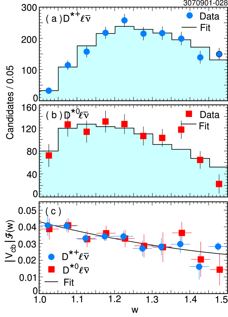
Figure 18: The results of the combined fit to the $w$ distribution: (a) the $D^{*+}\ell\bar{\nu}$ yields (circles) with the results of the fit superimposed (histogram) and (b) the $D^{*0}\ell\bar{\nu}$ yields (squares) and fit (histogram). In (c) the curve shows the best-fit $|V_{cb}|{\cal F}(w)$, and the circles (squares) are the $D^{*+}\ell\bar{\nu}$ ($D^{*0}\ell\bar{\nu}$) yields corrected for efficiency, smearing, and all terms in the differential decay rate apart from $|V_{cb}|{\cal F}(w)$.

These results may be compared to our previous analysis oldcleo that analyzed a subset (approximately 50%) of the current data finding a smaller value for $|V_{cb}|{\cal F}(1)$. The increase may be attributed to several effects. Changes in the measured values of the $D^{0}$ and $D^{*}$ branching fractions and $B$ lifetimes cause a 2.3% increase. Inclusion of final-state radiation shifts $|V_{cb}|{\cal F}(1)$ by 2.4%. More significantly, use of the improved form factor gives an increase of 5.7%. The new form factor has positive curvature, which results in an increase when extrapolating to $w=1$. The analysis of Caprini et al. caprini shows there is correlation between the curvature and slope of the form factor, making this effect more pronounced for the large slope preferred by our data. The remainder of the increase results from the larger data sample.

We test the compatibility of the old and new analyses by restricting the new analysis to the same subset of data and fitting using the old form factor. Adjusting for common values for $D^{0}$ and $D^{*}$ branching fractions and $B$ lifetimes (Table 7) we find a change in $|V_{cb}|{\cal F}(1)$ of $0.0020\pm 0.0010\pm 0.0022$, where the first error is statistical (assessed conservatively assuming all candidates in the old analysis are found in the new analysis) and the second error is an estimate of the uncorrelated systematic uncertainties. The largest of the latter are due to slow pion efficiency, taken to be uncorrelated because of significant differences in the tracking algorithms used in the two analyses. We conclude the old and new analyses are compatible within the systematic uncertainties. Because our new analysis includes the data reported previously and takes advantage of theoretical improvements in the form factor, the results reported here supersede our previous results.

VI Systematic Uncertainties

The systematic uncertainties are summarized in Table 8. The dominant systematic uncertainties arise from our background estimations and from our knowledge of the slow pion reconstruction efficiency.

Table 8: The fractional systematic uncertainties, given in percent, for the $\bar{B^{0}}\to D^{*+}\ell\bar{\nu}$ fit, the $B^{-}\to D^{*0}\ell\bar{\nu}$ fit, and the combined fit.

	$D^{*+}\ell\bar{\nu}$ fit			$D^{*0}\ell\bar{\nu}$ fit			Combined fit
Source	$|V_{cb}|{\cal F}(1)$	$\rho^{2}$	$\Gamma$	$|V_{cb}|{\cal F}(1)$	$\rho^{2}$	$\Gamma$	$|V_{cb}|{\cal F}(1)$	$\rho^{2}$	$\Gamma$
Backgrounds	$1.8$	$3.0$	$1.8$	$2.4$	$5.0$	$2.2$	$1.8$	$3.1$	$1.7$
Reconstruction efficiency	$4.4$	$5.0$	$4.9$	$3.5$	$6.2$	$6.5$	$2.9$	$3.2$	$4.6$
$B$ momentum & mass	$0.2$	$0.0$	$0.5$	$0.6$	$0.5$	$0.8$	$0.1$	$0.1$	$0.2$
$\bar{B}\to D^{*}X\ell\bar{\nu}$ model	$0.3$	$3.5$	$1.2$	$1.2$	$2.7$	$0.5$	$0.3$	$1.6$	$0.9$
Final-state radiation	$0.7$	$0.3$	$1.1$	$0.8$	$0.5$	$1.2$	$0.7$	$0.3$	$1.1$
Number of $B\bar{B}$ events	$0.9$	$0.0$	$1.8$	$0.9$	$0.0$	$1.8$	$0.9$	$0.0$	$1.8$
Subtotal	$4.9$	$6.8$	$5.8$	$4.6$	$8.5$	$7.3$	$3.6$	$4.8$	$5.4$
$\tau_{B}$ and branching fractions	$1.5$	$0.0$	$3.0$	$2.8$	$0.0$	$5.6$	$1.8$	$0.0$	$3.5$
$R_{1}(1)$ and $R_{2}(1)$	$1.6$	$11.7$	$1.8$	$1.1$	$14.3$	$1.8$	$1.4$	$12.0$	$1.8$
Subtotal	$2.2$	$11.7$	$3.5$	$3.0$	$14.3$	$5.9$	$2.3$	$12.0$	$3.9$
Total	$5.3$	$13.5$	$6.8$	$5.5$	$16.6$	$9.3$	$4.3$	$13.0$	$6.6$

VI.1 Background uncertainties

Here we present the systematic uncertainties from our backgrounds.

VI.1.1 Continuum background

Our estimate of background from $e^{+}e^{-}\to q{\bar{q}}$ is taken from data collected below the $\Upsilon(4S)$. The shape of this background in each $w$ bin is taken from off-resonance data, where we scale the energy of the $D^{*}$ and lepton to reflect the difference in the on- and off-resonance center-of-mass energies. This scaling applies to computation of $w$ and $\cos\theta_{B-D^{*}\ell}$. The resulting distribution is scaled by the ratio $({\cal L}_{\text{on}}/{\cal L}_{\text{off}})(E_{\text{off}}^{2}/E_{\text{on}}^{2})$, where the first factor is the ratio of on- to off-resonance luminosities and the $E^{2}$ ratio corrects for the $1/s$ dependence of the hadronic cross section.

The uncertainty on the normalization is small and has negligible effect on the results because the continuum background itself is small. To assess the systematic uncertainty from the $D^{*}$ and lepton energy scaling, we compare our results with the scaling to those obtained without it. The systematic uncertainties are taken to be half this difference, and are 0.03%, 0.2%, and 0.1% for $|V_{cb}|{\cal F}(1)$, $\rho^{2}$, and $\Gamma(\bar{B}\to D^{*}\ell\bar{\nu})$, respectively.

VI.1.2 Combinatoric background

Our method for combinatoric background subtraction assumes that the $\cos\theta_{B-D^{*}\ell}$ distribution of candidates in the $\Delta m$ sideband matches that of those in the signal region. The Monte Carlo simulation should reproduce any differences well since they arise from kinematic effects. We use a sample of 16 million Monte Carlo-simulated inclusive $B\bar{B}$ events to test this assumption. (See also Figs. 9 and 10 and discussion in Section IV.2.2.) We perform our analysis on the simulated events twice, once using the combinatoric background subtraction procedure outlined in Section IV.2.2 and once using the absolutely normalized “true” combinatoric background, i.e., $D^{*}$ candidates in the $\Delta m$ signal region that do not arise from the decay of a $D^{*}$, in place of the $\Delta m$ sideband distribution. Use of the “true” background instead of the estimate results in a shift in the combined fit of $(-1.3\pm 0.9)$% in $|V_{cb}|{\cal F}(1)$, $(-2.6\pm 1.3)$% in $\rho^{2}$, and $(-0.6\pm 0.9)$% in $\Gamma$. Any bias from the use of the $\Delta m$ sideband to estimate the combinatoric background is smaller than the statistical uncertainty of the fit to the data. We conservatively assign systematic errors equal to the quadrature sum of the shift and its statistical uncertainty, a total of 1.6% for $|V_{cb}|{\cal F}(1)$.

The normalization of the background relies on the fits to the $\Delta m$ distributions. We assign an uncertainty for this by repeating our analysis with different functional forms used to fit $\Delta m$. We also include a 0.1% uncertainty because the simulated $\Delta m$ signal peaks are shifted a few tenths of an MeV lower than the data. The statistical error on the background normalization is included in the statistical errors on our result.

The final contribution to the systematic uncertainty from our combinatoric background estimate comes from the decay modes other than $D\to K\pi$ that are reconstructed in our $m(K\pi)$ signal region. The specific modes were given in Table 4. We find the total contribution to our $D^{*}\ell\bar{\nu}$ yield from this source is (0.5$\pm$0.3)%. We add the yield and its uncertainty in quadrature to get a 0.6% uncertainty on our $D^{*}\ell\bar{\nu}$ yield. Because $|V_{cb}|{\cal F}(1)$ is proportional to the amplitude rather than the rate, its error is half as big. We find the total error on $|V_{cb}|{\cal F}(1)$ due to the combinatoric background to be 1.6%. The errors from all components are summarized in Table 9.

Table 9: The uncertainties due to the combinatoric background.

Variation	$|V_{cb}|{\cal F}(1)$ (%)	$\rho^{2}$(%)	$\Gamma(\bar{B}\to D^{*}\ell\bar{\nu})$(%)
$D^{*+}\ell\bar{\nu}$ fit
$\cos\theta_{B-D^{*}\ell}$ distribution of sideband candidates	1.6	2.7	1.3
$\Delta m$ sideband normalizations	0.2	0.3	0.3
Non-$K\pi$ decays(see Table 4)	0.3	0.0	0.6
Total	1.6	2.7	1.4
$D^{*0}\ell\bar{\nu}$ fit
$\cos\theta_{B-D^{*}\ell}$ distribution of sideband candidates	2.2	4.8	1.5
$\Delta m$ sideband normalizations	0.3	0.6	1.2
Non-$K\pi$ decays(see Table 4)	0.3	0.0	0.6
Total	2.2	4.9	2.0
combined fit
$\cos\theta_{B-D^{*}\ell}$ distribution of sideband candidates	1.6	2.9	1.1
$\Delta m$ sideband normalizations	0.2	0.3	0.6
Non-$K\pi$ decays(see Table 4)	0.3	0.0	0.6
Total	1.6	2.9	1.3

VI.1.3 Uncorrelated background

The main source of uncertainty from the uncorrelated background is the normalization of the various contributions. Of these, the most important is the normalization of the upper-vertex $D^{*}$ decays, which we vary by 50%. Smaller uncertainties arise from the primary and secondary lepton rates, the uncertainty in $B^{0}-\bar{B}^{0}$ mixing, and the uncertainty in the rate of exchanging $K$ and $\pi$ particles in $D^{*0}$ candidates. The effects of varying these rates are summarized in Table 10. The systematic uncertainties from the uncorrelated background estimate are at or below the 1% level.

Table 10: The systematic uncertainties for the uncorrelated background in the separate $D^{*+}\ell\bar{\nu}$ and $D^{*0}\ell\bar{\nu}$ fits and the combined fit. The upper-vertex contribution, the lepton normalizations, and $\chi_{d}$ are treated as completely correlated between the two modes; all others are uncorrelated.

Variation	$|V_{cb}|{\cal F}(1)$(%)	$\rho^{2}$(%)	$\Gamma(\bar{B}\to D^{*}\ell\bar{\nu})$(%)
$D^{*+}\ell\bar{\nu}$ fit
Upper-vertex $D^{*}$	0.7	0.9	0.4
Other	0.2	0.2	0.3
Total	0.7	1.0	0.5
$D^{*0}\ell\bar{\nu}$ fit
Upper-vertex $D^{*}$	0.6	0.9	0.4
Other	0.5	0.8	0.3
Total	0.8	1.2	0.5
Combined fit
Upper-vertex $D^{*}$	0.6	0.9	0.4
Other	0.3	0.3	0.3
Total	0.7	1.0	0.5

VI.1.4 Correlated background

We assess the uncertainty arising from the correlated background by varying the branching fractions of the contributing modes simultaneously by 50%. Since this is a small background, this variation has little effect on $|V_{cb}|{\cal F}(1)$, and the uncertainties are 0.1%, 0.6%, and 0.8% on $|V_{cb}|{\cal F}(1)$, $\rho^{2}$, and $\Gamma(\bar{B}\to D^{*}\ell\bar{\nu})$, respectively.

VI.1.5 Fake lepton background

We vary the measured electron and muon fake rates separately by 50%. This is conservative, but it has also almost no effect on our result; the total uncertainty on $|V_{cb}|{\cal F}(1)$ is 0.02%, while the uncertainties on $\rho^{2}$ and $\Gamma(\bar{B}\to D^{*}\ell\bar{\nu})$ are 0.3% and 0.2%, respectively.

VI.2 Slow $\pi$ reconstruction uncertainty

The largest source of uncertainty for the analysis is the efficiency for reconstructing the slow pion from the $D^{*}$ decay. Because of the small energy release in $D^{*}$ decays, the daughter pion has low momentum and travels approximately in the direction of the parent $D^{*}$. For our signal decays, the momentum range of the slow pion is 0 to about 250 MeV/$c$. Note also that $w=E_{D^{*}}/m_{D*}$ in the $B$ rest frame, so the slow-pion momentum is correlated with $w$ [see Fig. 19(a)].

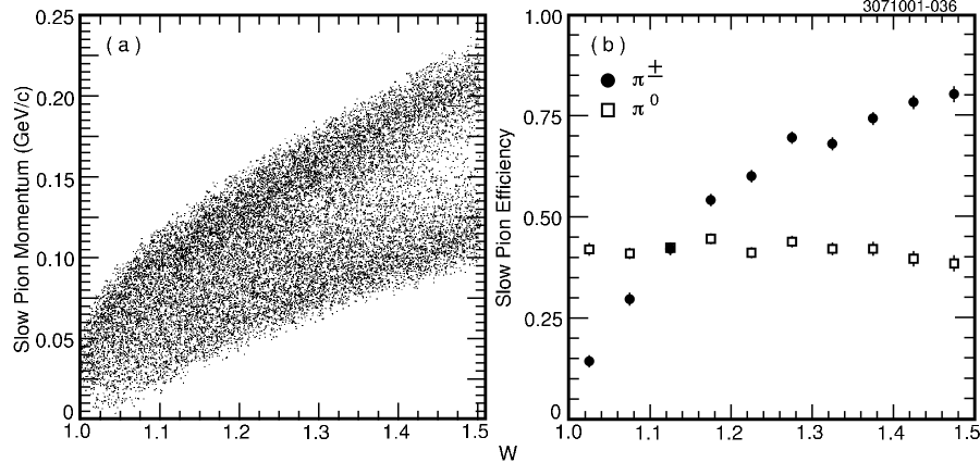
Figure 19: (a) The correlation between the slow pion momentum and $w$; (b) The reconstruction efficiency as a function of $w$ for charged slow pions (solid circles) and neutral slow pions (open squares).

Charged and neutral slow-pion reconstruction efficiencies depend very differently on $w$. Charged pions with momenta less than 50 MeV$/c$ do not penetrate far enough into the tracking chamber to be reconstructed; the slow-pion reconstruction efficiency is therefore low near $w=1$ and increases rapidly over the next few $w$ bins as the pion momentum increases. Neutral slow pions, on the other hand, decay to two low-energy photons (30–230 MeV). The lowest-momentum $\pi^{0}$’s decay almost back-to-back, depositing about equal energy in the calorimeter. As the $\pi^{0}$ momentum increases, the Lorentz boost pushes some of the photons below our minimum energy requirement of 30 MeV. The neutral slow-pion efficiency therefore drops slowly as $w$ increases. The slow-pion efficiencies for both charged and neutral $\pi$’s from $\bar{B}\to D^{*}\ell\bar{\nu}$ decays are shown as a function of $w$ in Fig. 19(b).

Because we rely on Monte Carlo simulation to estimate the slow-pion efficiencies, we investigate possible differences between the simulation and performance of the CLEO detector in order to estimate the systematic uncertainty of slow-pion reconstruction. We consider the effect of nearby tracks and showers on slow-pion reconstruction, comparing the efficiency of data and Monte Carlo-simulated $B\bar{B}$ events to limit a systematic error due to a difference in the “event environment” in data and simulated events. We also consider how much imperfect knowledge of detector material can affect reconstruction efficiency through pion range-out, multiple scattering, hadronic interaction, or photon conversions. Finally, we vary parameters of the detector simulation for the drift chambers and calorimeter to estimate the contribution to the systematic uncertainty.

Monte Carlo-simulated events may have a different number of drift chamber hits or calorimeter showers than the data. The detector activity (track fragments or showers) near a candidate slow pion can affect the reconstruction efficiency. To evaluate the impact of these “environment effects” on the slow-pion reconstruction efficiency, we insert Monte Carlo-generated slow-pion tracks or showers with kinematic distributions appropriate to $D^{*}\ell\bar{\nu}$ decay into samples of hadronic events selected from our data and from simulated $B\bar{B}$ events. In each $w$ bin, we compare the reconstruction efficiency for the tracks embedded into data and simulated events. For $D^{*+}\ell\bar{\nu}$, the efficiency difference is small, $\Delta\epsilon/\epsilon=(0.2\pm 1.1)$% integrated over $w$. Likewise, the effect of event environment is small for $D^{*0}\ell\bar{\nu}$, where we find a net efficiency difference $\Delta\epsilon/\epsilon=(-0.6\pm 1.1)$%. The uncertainties here are from the statistics of the data and Monte Carlo comparison. We measure the impact of the event environment by using the measured data-Monte Carlo efficiency difference in each $w$ bin to modify the efficiency matrix in Eq. 13 and repeating the fit. The slow-pion efficiency may depend on the track or shower multiplicity, which is increased by one or two, respectively, by the embedding study; we find no statistically significant evidence of this in our studies, but we include a small uncertainty [0.3% on $|V_{cb}|{\cal F}(1)$] to cover this effect.

To estimate the uncertainty due to our imperfect knowledge of the detector material inside the outer boundary of the tracking chambers, we vary the material description of the detector by 10% in our simulation and remeasure the slow-pion efficiencies. This 10% variation of material is based on a study that compared the polar angle distribution of $e^{+}e^{-}\to\gamma\gamma$ events in data and simulation. We then repeat the $|V_{cb}|$ fit using these new efficiencies and take the excursions of $|V_{cb}|{\cal F}(1)$, $\rho^{2}$, and $\Gamma(\bar{B}\to D^{*}\ell\bar{\nu})$ as the uncertainty.

In a similar way, we estimate the uncertainty due to our tracking chamber and crystal calorimeter simulation. For charged slow pions, performance of the tracking devices is essential. Differences in hit efficiency and single-hit resolution between data and Monte Carlo simulation can result in a difference in measured efficiency. The tracking simulation parameters are tuned using an independent sample of charged tracks. We vary the tracking chamber hit resolutions by amounts determined from residual distributions in these data, and we vary hit efficiencies according to observed differences in the data and simulated hit efficiencies.

For neutral slow pions, performance of the calorimeter is important. Here we consider differences in the $m(\gamma\gamma)$ and transverse shower profile distributions used for $\pi^{0}$ reconstruction. We calibrate the calorimeter energy scale at high energy (1–5 GeV) using showers from QED event samples ($e^{+}e^{-}\to e^{+}e^{-}$, $e^{+}e^{-}\to\gamma\gamma$, and $e^{+}e^{-}\to e^{+}e^{-}\gamma$). We check this scale with a sample of $\pi^{0}\to\gamma\gamma$ and $\eta\to\gamma\gamma$ candidates, which should peak at the known $\pi^{0}$ and $\eta$ masses. For low-energy showers there can be residual gain mismatches from nonlinearities and noise. Accordingly, we adjust the calorimeter noise and dispersion of crystal gains in the simulation so that it reproduces the transverse spatial distributions of the photon showers and the $m(\gamma\gamma)$ distribution for an independent sample of low-momentum $\pi^{0}$’s. We vary the noise and gain dispersion parameters in the simulation within a range determined from the data to assess the systematic uncertainty. Photons that convert and begin to shower just in front of the calorimeter will have degraded resolution. We vary the material description between the outer tracking chamber boundary and the calorimeter crystals by a conservative 15% to determine its contribution to the uncertainty for slow-$\pi^{0}$ reconstruction. The transverse spatial extent of photon showers varies with the low-energy cutoff in the shower simulation. To assess the uncertainty from the cutoff in our simulation, we lower the minimum energy for photon simulation by a factor of 10, from 1 MeV to 100 keV.

Finally, we assess the systematic uncertainty due to requiring a $D^{*+}$ and $D^{0}$ vertex in the $D^{*+}\ell\bar{\nu}$ analysis by performing the analysis without vertexing. In the separate $D^{*+}\ell\bar{\nu}$ fit without vertexing, the result for $|V_{cb}|{\cal F}(1)$ shifts by $(2.0\pm 1.8)$%, where the uncertainty takes into account correlations between analyses with and without vertexing. We take the quadrature sum of the shift and its uncertainty as a systematic error.

We find that the largest contributions to the uncertainty on $|V_{cb}|{\cal F}(1)$ come from the material description (1.3%), the effects of vertexing (1.5%), and the minimum energy for photon simulation (0.6%). The statistical uncertainty from data and Monte Carlo comparisons also contributes (1.3%). The given uncertainties apply to the combined fit. Table 11 summarizes the uncertainties on slow-pion reconstruction.

Table 11: The systematic errors from the slow-pion reconstruction efficiency for the separate $D^{*+}\ell\bar{\nu}$ and $D^{*0}\ell\bar{\nu}$ fits and the combined fit. We take the uncertainty from the material description to be correlated between the two modes; all other errors are uncorrelated.

Mode	$|V_{cb}|{\cal F}(1)$(%)	$\rho^{2}$(%)	$\Gamma(\bar{B}\to D^{*}\ell\bar{\nu})$(%)
$D^{*+}\ell\bar{\nu}$ fit
Material description	2.6	3.2	2.1
Tracking chamber hit efficiency	0.6	0.2	1.4
Vertexing	2.7	2.7	2.9
Other uncertainties	0.8	1.1	0.7
Statistics (environment)	1.7	2.5	1.4
Total	4.2	5.0	4.1
$D^{*0}\ell\bar{\nu}$ fit
Material description	1.1	3.0	0.6
Photon cutoff	1.5	0.9	2.3
Other uncertainties	1.2	2.9	5.0
Statistics (environment)	2.1	3.3	2.7
Total	3.1	5.4	6.2
Combined fit
Material description	1.3	1.5	1.2
Tracking chamber hit efficiency ($D^{*+}\ell\bar{\nu}$ only)	0.3	0.2	0.9
Vertexing ($D^{*+}\ell\bar{\nu}$ only)	1.5	1.6	1.7
Photon cutoff ($D^{*0}\ell\bar{\nu}$ only)	0.6	0.2	0.9
Other uncertainties	0.9	1.0	1.8
Statistics (environment)	1.3	2.1	1.3
Total	2.6	3.1	3.3

VI.3 Sensitivity to $R_{1}(1)$ and $R_{2}(1)$

The form factor ratios $R_{1}(1)$ and $R_{2}(1)$ affect the lepton spectrum and therefore the fraction of decays satisfying our 0.8 GeV/$c$ electron and 1.4 GeV/$c$ muon momentum requirements. They also affect the relative contributions of the three $D^{*}\ell\bar{\nu}$ form factors, and therefore can affect the form-factor slope $\rho^{2}$.

To estimate the uncertainty due to the measurement errors on $R_{1}(1)$ and $R_{2}(1)$, we use

$$\sigma_{P}^{2}=\sum_{i,j=1}^{2}\frac{\partial P}{\partial R_{i}(1)}\frac{\partial P}{\partial R_{j}(1)}E_{ij},$$ (17)

where $P$ stands for the parameter [$|V_{cb}|{\cal F}(1)$, $\rho^{2}$, or $\Gamma(\bar{B}\to D^{*}\ell\bar{\nu})$] whose uncertainty we are calculating, $E_{ii}=\sigma_{i}^{2}$ and $E_{ij}=\rho_{ij}\sigma_{i}\sigma_{j}$, where $\rho_{12}=-0.82$ is the correlation coefficient from the $R_{1}(1)$ and $R_{2}(1)$ measurement ffprl . We compute the partial derivatives $\partial P/\partial R_{i}(1)$ by shifting $R_{i}$ and repeating our analysis. We find an uncertainty on $|V_{cb}|{\cal F}(1)$ from this source of 1.4%, and a substantial uncertainty on $\rho^{2}$ of 12%.

VI.4 Other uncertainties

We considered the following minor sources of systematic uncertainty, summarized in Table 8.

The efficiency for identifying electrons has been evaluated using radiative Bhabha events embedded in hadronic events, and has an uncertainty of 2.6%. Similarly, the muon identification efficiency has been evaluated using radiative mu-pair events, and has an uncertainty of 1.6%. We determine the total uncertainty from lepton identification by adding in quadrature the shift in results when repeating the analysis with electron and muon efficiencies varied by their momentum-dependent uncertainties. Separate electron and muon analyses of our data give the results shown in Table 12. Including the systematic uncertainties on lepton identification, the separate electron and muon results are consistent at the 35% confidence level.

Table 12: The results from separate analyses using only $D^{*}e^{-}\bar{\nu}$ or $D^{*}\mu^{-}\bar{\nu}$. The errors are statistical only. In these fits $f_{+-}$ is constrained using Ref. sylvia, .

Mode	$|V_{cb}|{\cal F}(1)$(%)	$\rho^{2}$(%)	$\Gamma(\bar{B}\to D^{*}\ell\bar{\nu})$(%)
$D^{*+}\ell\bar{\nu}$
$D^{*+}e^{-}\bar{\nu}$	0.0420$\pm$0.0023	1.65$\pm$0.14	0.0363$\pm$0.0021
$D^{*+}\mu^{-}\bar{\nu}$	0.0448$\pm$0.0026	1.69$\pm$0.15	0.0404$\pm$0.0025
$D^{*0}\ell\bar{\nu}$
$D^{*0}e^{-}\bar{\nu}$	0.0409$\pm$0.0032	1.41$\pm$0.24	0.0396$\pm$0.0030
$D^{*0}\mu^{-}\bar{\nu}$	0.0474$\pm$0.0040	1.80$\pm$0.26	0.0423$\pm$0.0042
combined
$D^{*}e^{-}\bar{\nu}$	0.0420$\pm$0.0018	1.60$\pm$0.12	0.0374$\pm$0.0015
$D^{*}\mu^{-}\bar{\nu}$	0.0457$\pm$0.0021	1.73$\pm$0.13	0.0411$\pm$0.0019

The $B$ momentum is measured directly in the data using fully reconstructed hadronic decays, and is known on average with a precision of 0.0016 GeV/$c$. Variation of the momentum in our reconstruction slightly alters the $\cos\theta_{B-D^{*}\ell}$ distribution that we expect for our signal, and it therefore changes the yields obtained from the $\cos\theta_{B-D^{*}\ell}$ fits. Likewise, CLEO has measured the $B^{0}$- and $B^{+}$-meson masses ershov and when we vary them within their measurement errors, we find a small effect on the yields.

We determine the tracking efficiency uncertainties for the lepton and the $K$ and $\pi$ forming the $D^{0}$ in the same study used for the slow pion from the $D^{*+}$ decay. These uncertainties are confirmed in a study of 1-prong versus 3-prong $\tau$ decay events from our data sample.

The final-state radiation model has a small effect on our $D^{*}\ell\bar{\nu}$ yields because it affects the $D^{*}\ell\bar{\nu}$ $\cos\theta_{B-D^{*}\ell}$ distributions. Because we require $p_{e}\geq 0.8$ GeV/$c$ and $p_{\mu}\geq 1.4$ GeV/$c$, the model also affects the $D^{*}\ell\bar{\nu}$ efficiency. The final-state radiation model is estimated by the authors of Photos to be accurate within 30% photos . We determine our sensitivity to the model by repeating our analysis without including radiative $D^{*}\ell\bar{\nu}$ decays in our $D^{*}\ell\bar{\nu}$ Monte Carlo. We then take 30% of the change to our results as our uncertainty.

Finally, our analysis requires that we know the $\cos\theta_{B-D^{*}\ell}$ distribution of the $D^{*}X\ell\bar{\nu}$ contribution. This distribution in turn depends on both the branching fractions of contributing modes and on their form factors. Variation of all of these branching fractions and form factors is not only cumbersome, but also out of reach given the poor current knowledge of these modes. Instead, we note that the $\bar{B}\to D^{*}\pi\ell\bar{\nu}$ and $\bar{B}\to D_{1}\ell\bar{\nu}$ modes are the ones with the most extreme $\cos\theta_{B-D^{*}\ell}$ distributions (the largest mean and the smallest). These distributions are shown in Fig. 20. We therefore repeat the analysis, first using only $\bar{B}\to D^{*}\pi\ell\bar{\nu}$ to describe our $D^{*}X\ell\bar{\nu}$ decays and then using only $\bar{B}\to D_{1}\ell\bar{\nu}$ to describe these decays; we take the larger of the two excursions as our systematic error.

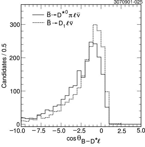
Figure 20: The $\cos\theta_{B-D^{*}\ell}$ distribution of $\bar{B}\to D^{*0}\pi\ell\bar{\nu}$ (solid histogram) and $\bar{B}\to D_{1}\ell\bar{\nu}$ (dashed histogram) decays contributing to the $D^{*}X\ell\bar{\nu}$ sample for $D^{*0}\ell\bar{\nu}$. The histograms are normalized to equal area.

VII Conclusions

We have fit the $w$ distribution of $\bar{B}\to D^{*}\ell\bar{\nu}$ decays for the slope of the form factor and $|V_{cb}|{\cal F}(1)$. For the combined $D^{*+}\ell\bar{\nu}$ and $D^{*0}\ell\bar{\nu}$ fit, we find

$$|V_{cb}|{\cal F}(1) = 0.0431\pm 0.0013\pm 0.0018,\ {\text{and}}$$

$$\rho^{2} = 1.61\pm 0.09\pm 0.21.$$

Including the systematic uncertainties we compute a correlation coefficient $C(|V_{cb}|{\cal F}(1),\rho^{2})=0.22$. Figure 21 shows the total error ellipse for this measurement. The best-fit parameters imply the decay rate

$$\Gamma=0.0394\pm 0.0012\pm 0.0026\ \text{ps}^{-1}.$$

We recover the branching fractions from the rate by dividing by the appropriate $B$-meson lifetimes. These results are sensitive only to the ratio of $B^{+}$ to $B^{0}$ lifetimes. They are

$${\cal B}(\bar{B^{0}}\to D^{*+}\ell\bar{\nu}) = (6.09\pm 0.19\pm 0.40)\%{\ \text{and}}$$

$${\cal B}(B^{-}\to D^{*0}\ell\bar{\nu}) = (6.50\pm 0.20\pm 0.44)\%,$$

where the errors are completely correlated.

A recent lattice calculation yields kronfeld ${\cal F}(1)=0.919^{+0.030}_{-0.035}$ after applying a QED correction of $+0.007$. This value is consistent with ${\cal F}(1)=0.913\pm 0.042$, the evaluation of the authors of Ref. babarbook, , but is more precise. Using the lattice value of ${\cal F}(1)$, our result implies

$$|V_{cb}|=0.0469\pm 0.0014\text{(stat.)}\pm 0.0020\text{(syst.)}\pm 0.0018\text{(theo.)}.$$

Since full radiative corrections have yet to be calculated for ${\cal F}(1)$, it is ambiguous how best to treat radiative decays in the analysis. We include radiative decays in our signal.

This value of $|V_{cb}|$ is consistent with previous values obtained from $D^{*}\ell\bar{\nu}$ decays aleph_dslnu ; opal_dslnu ; delphi_dslnu ; belle_dslnu , but is somewhat higher. However, we note our ability to reconstruct $\cos\theta_{B-D^{*}\ell}$ makes our analysis approximately four times less sensitive to the poorly known $D^{*}X\ell\bar{\nu}$ background, and furthermore allows us to constrain it with the data. This value of $|V_{cb}|$ is also somewhat higher than that obtained using inclusive semileptonic $B$ decays cleomoments . If confirmed, this discrepancy could signal a violation of quark-hadron duality. A larger value of $|V_{cb}|$ shifts constraints on the CKM unitarity triangle from $|V_{ub}/V_{cb}|$ and $CP$ violation in the neutral kaon system, somewhat reducing expectations for indirect $CP$ violation in the $B$ system.

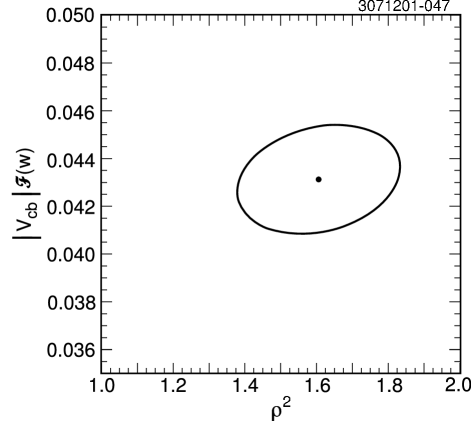
Figure 21: The error ellipse for the combined $D^{*+}\ell\bar{\nu}$ and $D^{*0}\ell\bar{\nu}$ measurement, including statistical and systematic uncertainties.

- (1) N. Cabibbo, Phys. Rev. Lett. 10, 531 (1963).
- (2) M. Kobayashi and T. Maskawa, Prog. Theor. Phys. 49, 652 (1973).
- (3) L. -L. Chau and W. -Y. Keung, Phys. Rev. Lett. 53, 1802 (1984); J. D. Bjorken, Phys. Rev. D 39, 1396 (1989); C. Jarlskog and R. Stora, Phys. Lett. B 208, 268 (1988); J. L. Rosner, A. I. Sanda, and M. P. Schmidt, in Proceedings of the Workshop on High Sensitivity Beauty Physics at Fermilab. Fermilab, November 11-14, 1987, edited by A. J. Slaughter, N. Lockyer, and M. Schmidt (Fermilab, Batavia, 1988), p 165; C. Hamzaoui, J. L. Rosner, and A. I. Sanda, ibid., p 215.
- (4) See, for example, A. J. Buras, M. E. Lautenbacher, and G. Ostermaier, Phys. Rev. D 50, 3433 (1994).
- (5) M. B. Voloshin and M. A. Shifman, Sov. J. Nucl. Phys. 47, 511 (1988).
- (6) N. Isgur and M. B. Wise, Phys. Lett. B 232, 113 (1989); 237, 527 (1990).
- (7) M. E. Luke, Phys. Lett. B 252, 447 (1990).
- (8) A. F. Falk, H. Georgi, B. Grinstein, and M. B. Wise, Nuc. Phys. B343, 1 (1990).
- (9) M. Neubert, Phys. Lett. B 264, 455 (1991).
- (10) B. Grinstein, Nuc. Phys. B339, 253 (1990).
- (11) E. Eichten and F. Feinberg, Phys. Rev. D 23, 2724 (1981); E. Eichten and B. Hill, Phys. Lett. B 234, 511 (1990); 243, 427 (1990).
- (12) H. Georgi, Phys. Lett. B 240, 447 (1990).
- (13) J. G. Körner and G. Thompson, Phys. Lett. B 264, 185 (1991).
- (14) T. Mannel, W. Roberts, and Z. Ryzak, Nuc. Phys. B368, 204 (1992).
- (15) M. Neubert, Phys. Rev. D 46, 2212 (1992).
- (16) A. F. Falk and M. Neubert, Phys. Rev. D 47, 2965 (1993).
- (17) CLEO Collaboration, R. A. Briere et al., Phys. Rev. Lett. 89, 081803 (2002) [hep-ex/0202032].
- (18) CLEO Collaboration, B. Barish et al., Phys. Rev. D 51, 1014 (1995).
- (19) B. L. Valant-Spaight, Ph. D. thesis, Cornell University, 2001.
- (20) CLEO Collaboration, Y. Kubota et al., Nucl. Instrum. Methods Phys. Res., Sect. A 320, 66 (1992).
- (21) R. Brun et al., Geant 3.15, CERN DD/EE/84-1.
- (22) G. C. Fox and S. Wolfram, Phys. Rev. Lett. 41, 1581 (1978).
- (23) P. Billoir, Nucl. Inst. Meth. Res., Sect. A 255, 352 (1984).
- (24) CLEO Collaboration, S.E. Csorna et al., Phys. Rev. D 61, 111101 (2000) [hep-ex/0001013].
- (25) R. Barlow and C. Beeston, Comput. Phys. Commun. 77, 219 (1993).
- (26) I. Caprini, L. Lellouch, and M. Neubert, Nucl. Phys. B530, 153 (1998) [hep-ph/9712417].
- (27) E. Barberio and Z. Wa̧s, Comput. Phys. Commun. 79, 291 (1994).
- (28) D. Scora and N. Isgur, Phys. Rev. D 52, 2783 (1995); N. Isgur et al., Phys. Rev. D 39, 799 (1989).
- (29) J. L. Goity and W. Roberts, Phys. Rev. D 51, 3459 (1995).
- (30) D. E. Groom et al., Eur. Phys. J. C 15, 1 (2000).
- (31) CLEO Collaboration, CONF 97-26 (1997).
- (32) CLEO Collaboration, B. Barish et al., Phys. Rev. Lett. 76, 1570 (1996).
- (33) ALEPH Collaboration, D. Buskulic et al., Z. Phys. C 73, 601 (1997).
- (34) DELPHI Collaboration, P. Abreu et al., Phys. Lett. B 475, 407 (2000).
- (35) J. D. Richman and P. R. Burchat, Rev. Mod. Phys. 67, 893 (1995).
- (36) CLEO Collaboration, J. Duboscq et al., Phys. Rev. Lett. 76, 3898 (1996).
- (37) M. Neubert, Physics Reports, 245, 259 (1994).
- (38) C. G. Boyd, B. Grinstein, and R. F. Lebed, Phys. Rev. D 56, 6895 (1997) [hep-ph/9705252].
- (39) CLEO Collaboration, D. S. Akerib et al., Phys. Rev. Lett. 71, 3070 (1993).
- (40) ALEPH Collaboration, R. Barate et al., Phys. Lett. B 403, 367 (1997).
- (41) CLEO Collaboration, J. P. Alexander et al., Phys. Rev. Lett. 86, 2737 (2001), [hep-ex/0006002].
- (42) S. Hashimoto et al., Phys. Rev. D 66, 014503 (2002), [hep-ph/0110253].
- (43) BaBar Physics Book, edited by P. F. Harrison and H. R. Quinn, SLAC-R-504 (1998).
- (44) ALEPH Collaboration, D. Buskulic et al., Phys. Lett. B 395, 373 (1997).
- (45) OPAL Collaboration, G. Abbiendi et al., Phys. Lett. B 482, 15 (2000).
- (46) DELPHI Collaboration, P. Abreu et al., Phys. Lett. B 510, 55 (2001).
- (47) BELLE Collaboration, K. Abe et al., Phys. Lett. B 526, 258 (2002).
- (48) CLEO Collaboration, D. Cronin-Hennessy et al., Phys. Rev. Lett. 87, 251808 (2001), [hep-ex/0108033].