EUROPEAN ORGANIZATION FOR NUCLEAR RESEARCH

CERN-EP/2002-051

10 July 2002

revised version 26 March 2003

Inclusive Analysis of the b Quark Fragmentation Function in Z Decays at LEP

The OPAL Collaboration

Abstract

A study of $\mathrm{b}$ quark hadronisation is presented using inclusively reconstructed $\mathrm{B}$ hadrons in about four million hadronic $\mathrm{Z}$ decays recorded in 1992–2000 with the OPAL detector at LEP. The data are compared to different theoretical models, and fragmentation function parameters of these models are fitted. The average scaled energy of weakly decaying B hadrons is determined to be

$$\langle\mathit{x}_{\,\mathrm{E}}\rangle=0.7193\pm 0.0016(stat)^{+0.0038}_{-0.0033}(syst)\ .$$

(Submitted to Eur. Phys. J. C)

The OPAL Collaboration

G. Abbiendi², C. Ainsley⁵, P.F. Åkesson³, G. Alexander²², J. Allison¹⁶, P. Amaral⁹, G. Anagnostou¹, K.J. Anderson⁹, S. Arcelli², S. Asai²³, D. Axen²⁷, G. Azuelos^18,a, I. Bailey²⁶, E. Barberio⁸, R.J. Barlow¹⁶, R.J. Batley⁵, P. Bechtle²⁵, T. Behnke²⁵, K.W. Bell²⁰, P.J. Bell¹, G. Bella²², A. Bellerive⁶, G. Benelli⁴, S. Bethke³², O. Biebel³², I.J. Bloodworth¹, O. Boeriu¹⁰, P. Bock¹¹, D. Bonacorsi², M. Boutemeur³¹, S. Braibant⁸, L. Brigliadori², R.M. Brown²⁰, K. Buesser²⁵, H.J. Burckhart⁸, J. Cammin³, S. Campana⁴, R.K. Carnegie⁶, B. Caron²⁸, A.A. Carter¹³, J.R. Carter⁵, C.Y. Chang¹⁷, D.G. Charlton^1,b, I. Cohen²², A. Csilling^8,g, M. Cuffiani², S. Dado²¹, G.M. Dallavalle², S. Dallison¹⁶, A. De Roeck⁸, E.A. De Wolf⁸, K. Desch²⁵, M. Donkers⁶, J. Dubbert³¹, E. Duchovni²⁴, G. Duckeck³¹, I.P. Duerdoth¹⁶, E. Elfgren¹⁸, E. Etzion²², F. Fabbri², L. Feld¹⁰, P. Ferrari¹², F. Fiedler³¹, I. Fleck¹⁰, M. Ford⁵, A. Frey⁸, A. Fürtjes⁸, P. Gagnon¹², J.W. Gary⁴, G. Gaycken²⁵, C. Geich-Gimbel³, G. Giacomelli², P. Giacomelli², M. Giunta⁴, J. Goldberg²¹, E. Gross²⁴, J. Grunhaus²², M. Gruwé⁸, P.O. Günther³, A. Gupta⁹, C. Hajdu²⁹, M. Hamann²⁵, G.G. Hanson⁴, K. Harder²⁵, A. Harel²¹, M. Harin-Dirac⁴, M. Hauschild⁸, J. Hauschildt²⁵, C.M. Hawkes¹, R. Hawkings⁸, R.J. Hemingway⁶, C. Hensel²⁵, G. Herten¹⁰, R.D. Heuer²⁵, J.C. Hill⁵, K. Hoffman⁹, R.J. Homer¹, D. Horváth^29,c, R. Howard²⁷, P. Hüntemeyer²⁵, P. Igo-Kemenes¹¹, K. Ishii²³, H. Jeremie¹⁸, P. Jovanovic¹, T.R. Junk⁶, N. Kanaya²⁶, J. Kanzaki²³, G. Karapetian¹⁸, D. Karlen⁶, V. Kartvelishvili¹⁶, K. Kawagoe²³, T. Kawamoto²³, R.K. Keeler²⁶, R.G. Kellogg¹⁷, B.W. Kennedy²⁰, D.H. Kim¹⁹, K. Klein¹¹, A. Klier²⁴, S. Kluth³², T. Kobayashi²³, M. Kobel³, T.P. Kokott³, S. Komamiya²³, L. Kormos²⁶, R.V. Kowalewski²⁶, T. Krämer²⁵, T. Kress⁴, P. Krieger^6,l, J. von Krogh¹¹, D. Krop¹², M. Kupper²⁴, P. Kyberd¹³, G.D. Lafferty¹⁶, H. Landsman²¹, D. Lanske¹⁴, J.G. Layter⁴, A. Leins³¹, D. Lellouch²⁴, J. Letts¹², L. Levinson²⁴, J. Lillich¹⁰, S.L. Lloyd¹³, F.K. Loebinger¹⁶, J. Lu²⁷, J. Ludwig¹⁰, A. Macpherson^28,i, W. Mader³, S. Marcellini², T.E. Marchant¹⁶, A.J. Martin¹³, J.P. Martin¹⁸, G. Masetti², T. Mashimo²³, P. Mättig^m, W.J. McDonald²⁸, J. McKenna²⁷, T.J. McMahon¹, R.A. McPherson²⁶, F. Meijers⁸, P. Mendez-Lorenzo³¹, W. Menges²⁵, F.S. Merritt⁹, H. Mes^6,a, A. Michelini², S. Mihara²³, G. Mikenberg²⁴, D.J. Miller¹⁵, S. Moed²¹, W. Mohr¹⁰, T. Mori²³, A. Mutter¹⁰, K. Nagai¹³, I. Nakamura²³, H.A. Neal³³, R. Nisius⁸, S.W. O’Neale¹, A. Oh⁸, A. Okpara¹¹, M.J. Oreglia⁹, S. Orito²³, C. Pahl³², G. Pásztor^8,g, J.R. Pater¹⁶, G.N. Patrick²⁰, J.E. Pilcher⁹, J. Pinfold²⁸, D.E. Plane⁸, B. Poli², J. Polok⁸, O. Pooth¹⁴, M. Przybycień^8,j, A. Quadt³, K. Rabbertz⁸, C. Rembser⁸, P. Renkel²⁴, H. Rick⁴, J.M. Roney²⁶, S. Rosati³, Y. Rozen²¹, K. Runge¹⁰, D.R. Rust¹², K. Sachs⁶, T. Saeki²³, O. Sahr³¹, E.K.G. Sarkisyan^8,j, A.D. Schaile³¹, O. Schaile³¹, P. Scharff-Hansen⁸, J. Schieck³², T. Schoerner-Sadenius⁸, M. Schröder⁸, M. Schumacher³, C. Schwick⁸, W.G. Scott²⁰, R. Seuster^14,f, T.G. Shears^8,h, B.C. Shen⁴, C.H. Shepherd-Themistocleous⁵, P. Sherwood¹⁵, G. Siroli², A. Skuja¹⁷, A.M. Smith⁸, R. Sobie²⁶, S. Söldner-Rembold^10,d, S. Spagnolo²⁰, F. Spano⁹, A. Stahl³, K. Stephens¹⁶, D. Strom¹⁹, R. Ströhmer³¹, S. Tarem²¹, M. Tasevsky⁸, R.J. Taylor¹⁵, R. Teuscher⁹, M.A. Thomson⁵, E. Torrence¹⁹, D. Toya²³, P. Tran⁴, T. Trefzger³¹, A. Tricoli², I. Trigger⁸, Z. Trócsányi^30,e, E. Tsur²², M.F. Turner-Watson¹, I. Ueda²³, B. Ujvári^30,e, B. Vachon²⁶, C.F. Vollmer³¹, P. Vannerem¹⁰, M. Verzocchi¹⁷, H. Voss⁸, J. Vossebeld⁸, D. Waller⁶, C.P. Ward⁵, D.R. Ward⁵, P.M. Watkins¹, A.T. Watson¹, N.K. Watson¹, P.S. Wells⁸, T. Wengler⁸, N. Wermes³, D. Wetterling¹¹ G.W. Wilson^16,k, J.A. Wilson¹, G. Wolf²⁴, T.R. Wyatt¹⁶, S. Yamashita²³, V. Zacek¹⁸, D. Zer-Zion⁴, L. Zivkovic²⁴

¹School of Physics and Astronomy, University of Birmingham, Birmingham B15 2TT, UK
²Dipartimento di Fisica dell’ Università di Bologna and INFN, I-40126 Bologna, Italy
³Physikalisches Institut, Universität Bonn, D-53115 Bonn, Germany
⁴Department of Physics, University of California, Riverside CA 92521, USA
⁵Cavendish Laboratory, Cambridge CB3 0HE, UK
⁶Ottawa-Carleton Institute for Physics, Department of Physics, Carleton University, Ottawa, Ontario K1S 5B6, Canada
⁸CERN, European Organisation for Nuclear Research, CH-1211 Geneva 23, Switzerland
⁹Enrico Fermi Institute and Department of Physics, University of Chicago, Chicago IL 60637, USA
¹⁰Fakultät für Physik, Albert-Ludwigs-Universität Freiburg, D-79104 Freiburg, Germany
¹¹Physikalisches Institut, Universität Heidelberg, D-69120 Heidelberg, Germany
¹²Indiana University, Department of Physics, Swain Hall West 117, Bloomington IN 47405, USA
¹³Queen Mary and Westfield College, University of London, London E1 4NS, UK
¹⁴Technische Hochschule Aachen, III Physikalisches Institut, Sommerfeldstrasse 26-28, D-52056 Aachen, Germany
¹⁵University College London, London WC1E 6BT, UK
¹⁶Department of Physics, Schuster Laboratory, The University, Manchester M13 9PL, UK
¹⁷Department of Physics, University of Maryland, College Park, MD 20742, USA
¹⁸Laboratoire de Physique Nucléaire, Université de Montréal,  Montréal, Québec H3C 3J7, Canada
¹⁹University of Oregon, Department of Physics, Eugene OR 97403, USA
²⁰CLRC Rutherford Appleton Laboratory, Chilton, Didcot, Oxfordshire OX11 0QX, UK
²¹Department of Physics, Technion-Israel Institute of Technology, Haifa 32000, Israel
²²Department of Physics and Astronomy, Tel Aviv University, Tel Aviv 69978, Israel
²³International Centre for Elementary Particle Physics and Department of Physics, University of Tokyo, Tokyo 113-0033, and Kobe University, Kobe 657-8501, Japan
²⁴Particle Physics Department, Weizmann Institute of Science, Rehovot 76100, Israel
²⁵Universität Hamburg/DESY, Institut für Experimentalphysik, Notkestrasse 85, D-22607 Hamburg, Germany
²⁶University of Victoria, Department of Physics, P O Box 3055, Victoria BC V8W 3P6, Canada
²⁷University of British Columbia, Department of Physics, Vancouver BC V6T 1Z1, Canada
²⁸University of Alberta, Department of Physics, Edmonton AB T6G 2J1, Canada
²⁹Research Institute for Particle and Nuclear Physics, H-1525 Budapest, P O Box 49, Hungary
³⁰Institute of Nuclear Research, H-4001 Debrecen, P O Box 51, Hungary
³¹Ludwig-Maximilians-Universität München, Sektion Physik, Am Coulombwall 1, D-85748 Garching, Germany
³²Max-Planck-Institute für Physik, Föhringer Ring 6, D-80805 München, Germany
³³Yale University, Department of Physics, New Haven, CT 06520, USA

^a and at TRIUMF, Vancouver, Canada V6T 2A3
^b and Royal Society University Research Fellow
^c and Institute of Nuclear Research, Debrecen, Hungary
^d and Heisenberg Fellow
^e and Department of Experimental Physics, Lajos Kossuth University, Debrecen, Hungary
^f and MPI München
^g and Research Institute for Particle and Nuclear Physics, Budapest, Hungary
^h now at University of Liverpool, Dept of Physics, Liverpool L69 3BX, UK
ⁱ and CERN, EP Div, 1211 Geneva 23
^j and Universitaire Instelling Antwerpen, Physics Department, B-2610 Antwerpen, Belgium
^k now at University of Kansas, Dept of Physics and Astronomy, Lawrence, KS 66045, USA
^l now at University of Toronto, Dept of Physics, Toronto, Canada
^m current address Bergische Universität, Wuppertal, Germany

1 Introduction

Hadronisation, the transition of quarks into hadrons, is a strong interaction phenomenon which cannot yet be calculated from first principles within QCD. Monte Carlo event generators are used instead which rely on phenomenological models of this process. To some extent these models can be distinguished from each other by the shape of the predicted hadron energy distribution. Hadronisation of heavy quarks leads to a significantly harder hadron energy spectrum than for lighter quarks [1]. Experimentally, heavy quark hadronisation is of special interest, because in this case the hadron containing the primary quark can easily be identified.

A precise measurement of the $\mathrm{B}$ hadron energy distribution allows the various hadronisation models available to be tested, and also helps to reduce one of the most important systematic uncertainties in many heavy flavour analyses. Earlier measurements of the $\mathrm{B}$ hadron energy distribution usually fell into one of three categories. 1) Some analyses were based on a measurement of the energy distribution of certain exclusive $\mathrm{B}$ hadron decays, mostly $\mathrm{B}\to\mathrm{D}^{*}\ell\nu$, to constrain the $\mathrm{B}$ hadron energy as precisely as possible [2, 3]. However, this leads to small candidate samples and thus to a large statistical uncertainty. 2) Other analyses attempted to increase the sample size by extracting the energy distribution of leptons from inclusive $\mathrm{B}\to\ell$ decays. Unfortunately the modelling of the lepton energy spectrum introduces large additional systematic uncertainties [4, 5]. 3) The most precise results so far have been achieved through the fully inclusive reconstruction of the $\mathrm{B}$ hadron energy [6]. The analysis presented here identifies $\mathrm{B}$ hadrons inclusively using secondary vertices.

2 Data sample and event selection

This analysis uses data taken at or near the $\mathrm{Z}$ resonance with the OPAL detector at LEP between 1992–2000. A detailed description of the OPAL detector can be found elsewhere [7]. The most important components of the detector for this analysis are the silicon microvertex detector, the tracking chambers, and the electromagnetic calorimeter. The microvertex detector consisted of two layers of silicon strip detectors which provided high spatial resolution near the interaction region. The central jet chamber was optimised for good spatial resolution in the plane perpendicular to the beam axis. The resolution along the beam direction was improved by the $z$ information delivered by the silicon microvertex detector (except in the first version present in 1992), by a vertex drift chamber between the silicon detector and the jet chamber, and by dedicated $z$-chambers surrounding the other tracking chambers. The central detector provided good double track resolution and precise determination of the momenta of charged particles by measuring the curvature of their trajectories in a magnetic field of $0.435\;$T. The solenoid was mounted outside the tracking chambers but inside the electromagnetic calorimeter, which consisted of approximately $12\thinspace 000$ lead glass blocks. The electromagnetic calorimeter was surrounded by a hadronic calorimeter and muon detectors.

Hadronic events are selected as described in Ref. [8], giving a hadronic $\mathrm{Z}$ selection efficiency of $(98.1\pm 0.5)\,\%$ and a background of less than $0.1\,\%$. Only data that were taken with the silicon microvertex detector in operation are used for this analysis. A data sample of about 3.91 million hadronic events is selected. This includes 0.41 million events taken for detector calibration purposes during the years 1996–2000, when LEP was operating at higher energies.

A total of 23.81 million Monte Carlo simulated events are used: 16.81 million events were generated with the JETSET 7.4 generator [9], 2 million events were generated with HERWIG 5.9 [10], and 5 million events were produced by HERWIG 6.2 [11]. The JETSET event sample includes 4.93 million $\mathrm{b}\overline{\mathrm{b}}$ events and 3.19 million $\mathrm{c}\overline{\mathrm{c}}$ events in dedicated heavy flavour samples. All other samples are mixed five flavour $\mathrm{Z}\to\mathrm{q}\overline{\mathrm{q}}$ event samples. The choice of important parameters of the event generators is described in [12]. All Monte Carlo simulated events are passed through a detailed detector simulation [13]. The same reconstruction algorithms as for data are applied to simulated events.

The analysis is performed separately for the data of different years, where detector upgrades, in particular of the silicon microvertex detector [14], and recalibrations lead to different conditions. Separate samples of JETSET Monte Carlo are available for all years. HERWIG Monte Carlo is only available for the largest homogeneous dataset taken in 1994, and therefore HERWIG-related studies are performed exclusively for this dataset.

In the 1993 and 1995 runs, part of the data was taken at centre-of-mass energies about $1.8\;\mathrm{GeV}$ above and below the peak of the $\mathrm{Z}$ resonance. The $\mathrm{B}$ hadron energy distribution is sensitive to energy losses due to initial state radiation prior to the annihilation process. Initial state radiation is heavily suppressed at and just below the $\mathrm{Z}$ resonance, but it has significant impact in the dataset taken at an energy of $m_{\mathrm{Z}}+1.8\;\mathrm{GeV}$. The latter samples are therefore treated separately, with Monte Carlo samples simulated for the appropriate energy, giving a total of eleven separate data and JETSET Monte Carlo samples.

3 Preselection of $\mathrm{Z}\to\mathrm{b}\overline{\mathrm{b}}$ events

The thrust axis is calculated for each event using tracks and electromagnetic clusters not associated with any tracks. To select events within the fiducial acceptance of the silicon microvertex detector and the barrel electromagnetic calorimeter, the thrust axis direction is required to satisfy $|\cos\theta_{T}|<0.8$, where $\theta_{T}$ is the thrust angle with respect to the beam direction.

To achieve optimal $\mathrm{b}$-tagging performance, each event is forced into a 2-jet topology using the Durham jet-finding scheme [15]. In calculating the visible energies and momenta of the event and of individual jets, corrections are applied to prevent double counting of energy in the case of tracks with associated clusters [16]. A $\mathrm{b}$-tagging algorithm is applied to each jet using three independent methods: lifetime tag, high $p_{t}$ lepton tag and jet-shape tag. This algorithm was developed for and used in the OPAL Higgs boson searches. A detailed description of the algorithm can be found in [17]. Its applicability to events recorded at the $\mathrm{Z}$ resonance peak was already shown in [18]. The $\mathrm{b}$-tagging discriminants calculated for each of the jets in the event are combined to yield an event $\mathrm{b}$ likelihood ${\cal B}_{\rm event}$. Both the jet b-tagging discriminant and ${\cal B}_{\rm event}$ have values between zero and one and correspond approximately to the probability of a true $\mathrm{b}$ jet or $\mathrm{b}\overline{\mathrm{b}}$ event, respectively. For each event, ${\cal B}_{\rm event}>0.2$ is required. The $\mathrm{Z}\to\mathrm{b}\overline{\mathrm{b}}$ event purity is 83% after this requirement, and the efficiency is 54% at this stage.

The $\mathrm{b}$ hemisphere tag efficiency obtained from Monte Carlo simulation is compared to the actual value in data using a double tag approach as described in [19]. The efficiencies obtained this way in both simulation and real data are found to agree to within 5% in all subsamples. Nevertheless a correction is applied to the Monte Carlo efficiency to further improve the agreement.

4 Reconstruction of $\mathrm{B}$ hadron energy

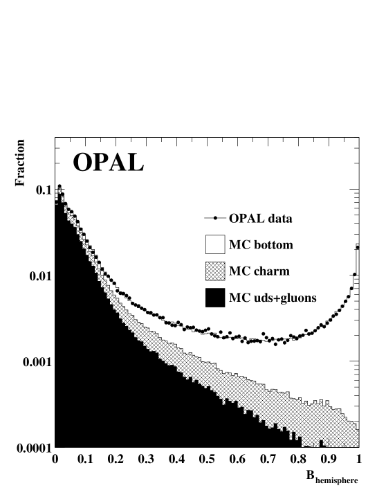
Figure 1: Distribution of the jet b-tagging discriminant in data (points with error bars) and Monte Carlo (histograms). The contributions from $\mathrm{b}$ jets, $\mathrm{c}$ jets, and light quark or gluon jets are shown as open, hatched, and black area respectively. Jets with a b-tagging discriminant above 0.8 in a jet in the opposite hemisphere are retained for analysis.

The primary event vertex is reconstructed using the tracks in the event constrained to the average position of the $\mathrm{e}^{+}\mathrm{e}^{-}$ collision point. For the $\mathrm{B}$ hadron reconstruction, tracks and electromagnetic calorimeter clusters with no associated track are combined into jets using a cone algorithm [20] with a cone half-angle of $0.65\rm\,rad$ and a minimum jet energy of $5.0\;\mathrm{GeV}$. The two most energetic jets of each event are assumed to contain the $\mathrm{B}$ hadrons. Only jets where the opposite hemisphere yields a $\mathrm{b}$-tagging discriminant of at least 0.8, corresponding to a $\mathrm{b}$ probability of about 80%, are used in the analysis. The distribution of the $\mathrm{b}$-tagging discriminant is shown in Figure 1.

Each remaining jet is searched for secondary vertices using a vertex reconstruction algorithm similar to that described in [21], making use of the tracking information in both the $r\phi$ and $rz$ planes where available. If a secondary vertex is found, the primary vertex is re-fitted excluding the tracks assigned to the secondary vertex. Secondary vertex candidates are accepted and called ‘good’ secondary vertices if they contain at least three tracks. If there is more than one good secondary vertex attached to a jet, the vertex with the largest number of significant tracks is taken. If there are two or more such vertices, the secondary vertex with the larger separation significance with respect to the primary vertex is taken. Jets without an associated secondary vertex are rejected. This increases the $\mathrm{b}$ jet purity and improves the energy resolution of the $\mathrm{B}$ hadron reconstruction described in the following.

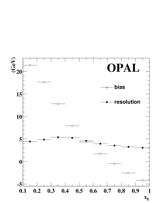
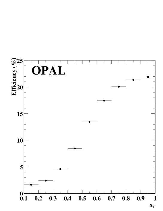
Figure 2: a) Dependence of the $\mathrm{B}$ hadron energy resolution (black circles) and reconstruction bias (open circles) on the generated $\mathrm{B}$ hadron energy. b) Dependence of the $\mathrm{B}$ hadron reconstruction efficiency on the generated $\mathrm{B}$ hadron energy.

Weakly decaying $\mathrm{B}$ hadrons are reconstructed inclusively with a method described in an earlier publication [22]. In each hemisphere defined by the positive axis of the jet found by the cone algorithm, a weight is assigned to each track and each cluster, where the weight corresponds to the probability that this track or cluster is a product of the $\mathrm{B}$ hadron decay. This weight is obtained from artificial neural networks [23] exploiting information from track impact parameters with respect to the primary and secondary vertices, and from kinematic quantities like the transverse momentum associated with a track or cluster, measured with respect to the cone jet axis. A list of all variables is shown in Table 1. The $\mathrm{B}$ hadron momentum is then reconstructed by summing the weighted momenta of the tracks and clusters. A beam energy constraint assuming a two-body decay of the $\mathrm{Z}$ and the world average $\mathrm{B}$ meson mass of $5.279\;\mathrm{GeV}/\mathit{c}^{\mathrm{2}}$ [24] for the $\mathrm{B}$ hadron is applied to improve the energy resolution. The constraints lead to a biased energy reconstruction, particularly when the true $\mathrm{B}$ hadron energy is very small, as can be seen in Figure 2a. However, only a small fraction of the data sample is in the low-energy region affected by a large bias. For most events, in the peak of the $\mathrm{B}$ hadron energy distribution, the bias is small, and all biases are taken into account by the fitting procedures used in both the model-dependent and model-independent analyses. Possible systematic uncertainties arising from the biased energy reconstruction are discussed in Section 7 of this paper. The energy of the weakly decaying $\mathrm{B}$ hadron is expressed in terms of the scaled energy $\mathit{x}_{\,\mathrm{E}}=E_{\mathrm{B}}/E_{beam}$, where $E_{beam}=\sqrt{s}/2$ is the LEP beam energy for the event. The quantity $\mathit{x}_{\,\mathrm{E}}$ is restricted to values above $5.279\;\mathrm{GeV}/E_{beam}\approx 0.1$ by the $\mathrm{B}$ meson mass constraint, and it cannot exceed 1.0 due to the beam energy constraint.

track neural network
track momentum
track rapidity with respect to estimated $\mathrm{B}$ hadron flight direction
track impact parameter with respect to primary vertex in $r\phi$ projection ($d_{0}$)
track impact parameter with respect to primary vertex in $z$ projection ($z_{0}$)
$d_{0}$ impact parameter significance
$z_{0}$ impact parameter significance
3d impact parameter significance with respect to the primary vertex
3d impact parameter significance with respect to the secondary vertex
cluster neural network
cluster energy
cluster rapidity with respect to estimated $\mathrm{B}$ hadron flight direction

Table 1: Variables used in artificial neural networks to estimate the probability that a track or calorimeter cluster originates from a $\mathrm{B}$ hadron decay. The impact parameter significance is defined as the impact parameter divided by its uncertainty.

After all these requirements, the distribution of the difference between the reconstructed energy and that of generated $\mathrm{B}$ hadrons in simulated data has a rms width of $4.8\;\mathrm{GeV}$. The energy dependence of the $\mathrm{B}$ hadron energy resolution is shown in Figure 2a. The complete $\mathrm{B}$ hadron selection applied to the full data sample results in $270\,707$ tagged jets with a $\mathrm{b}$ purity of 96%. The average $\mathrm{B}$ hadron selection efficiency is 16%, with an energy dependence as shown in Figure 2b. The measured $\mathrm{B}$ hadron energy distribution, scaled to the beam energy, is shown in Figures 3–6, and compared to the various models described in the next section.

5 Test of hadronisation models

fragmentation function	functional form	parameters
Kartvelishvili et al. [25]	$Nz^{\alpha_{\mathrm{b}}}(1-z)$	$\alpha_{\mathrm{b}}$
Bowler [26]	$N{1\over z^{1+bm_{\perp}^{2}}}(1-z)^{a}\exp(-{bm_{\perp}^{2}\over z})$	$a$, $bm_{\perp}^{2}$
Lund symmetric [27]	$N{1\over z}(1-z)^{a}\exp(-{bm_{\perp}^{2}\over z})$	$a$, $bm_{\perp}^{2}$
Peterson et al. [28]	$N{1\over z}(1-{1\over z}-{\varepsilon_{\mathrm{b}}\over 1-z})^{-2}$	$\varepsilon_{\mathrm{b}}$
Collins-Spiller [29]	$N({1-z\over z}+{(2-z)\varepsilon_{\mathrm{b}}\over 1-z})(1+z^{2})(1-{1\over z}-{\varepsilon_{\mathrm{b}}\over 1-z})^{-2}$	$\varepsilon_{\mathrm{b}}$

Table 2: Fragmentation functions for the JETSET 7.4 string scheme that are fitted to data in this paper. $N$ is a normalisation constant, different for each fragmentation function.

The $\mathrm{B}$ hadron energy distributions predicted by the JETSET 7.4, HERWIG 5.9, and HERWIG 6.2 Monte Carlo models are compared to the OPAL data. All Monte Carlo simulated events are passed through a detailed detector simulation [13]. The comparison is performed using the distribution of the reconstructed scaled energy of the weakly decaying $\mathrm{B}$ hadron $\mathit{x}_{\,\mathrm{E}}$.

The HERWIG Monte Carlo uses a parton shower fragmentation followed by cluster hadronisation model with few parameters. No parameters are varied in this analysis. This simplifies the model test to a mere comparison of the $\mathit{x}_{\,\mathrm{E}}$ distributions obtained with data and Monte Carlo simulation. Both HERWIG versions are set up to conserve the initial $\mathrm{b}$ quark direction in the $\mathrm{B}$ hadron creation during cluster decay (cldir=1). The main difference between the two HERWIG samples used in this analysis is that Gaussian smearing of the $\mathrm{B}$ hadron direction around the initial $\mathrm{b}$ quark flight direction is applied in the HERWIG 5.9 sample (clsmr=0.35), while smearing is not used in the HERWIG 6.2 sample (clsmr(2)=0).

The JETSET Monte Carlo is based on a parton shower fragmentation followed by string hadronisation scheme. It requires a fragmentation function to describe the distribution of the fraction $z$ of the string light cone momentum that is assigned to a hadron produced at the end of the string. The JETSET sample in this analysis is reweighted to use the fragmentation functions of Kartvelishvili et al. [25], Bowler [26], the Lund symmetric model [27], and the fragmentation functions of Peterson et al. [28], and Collins-Spiller [29]. The Lund symmetric and Bowler functions are simplified by assuming the transverse mass of the $\mathrm{b}$ quark, $m_{\perp}$, to be constant, which is justified by the smallness of the average transverse momentum compared to the $\mathrm{b}$ quark mass. A further simplification in the Bowler parametrisation is the assumption of an equality of $\mathrm{b}$ quark and hadron masses. The functional forms of the fragmentation functions are given in Table 2. The parameters of the respective fragmentation functions are fitted to obtain a best match of the observed $\mathit{x}_{\,\mathrm{E}}$ distributions in data and Monte Carlo simulation. In the case of the Peterson et al., Collins-Spiller, and Kartvelishvili et al. models, one free parameter is available. The Lund and Bowler models each have two free fit parameters. A $\chi^{2}$ fit is performed in 46 bins in the $\mathit{x}_{\,\mathrm{E}}$ range of 0.5 to 0.95, where in all samples the number of candidates in each bin is large enough to justify the assumption of Gaussian errors on the bin content. The fragmentation function and its parameters are adjusted during the fit by reweighting the Monte Carlo simulated events, similar to the procedure applied in [19].

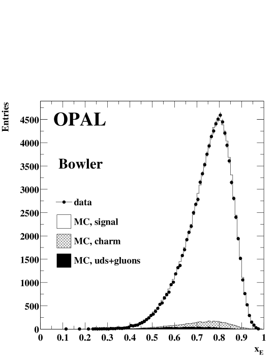
Figure 3: Results of the fit to the data of various hadronisation models for JETSET 7.4. The points with error bars are the uncorrected reconstructed scaled energy distribution in the 1994 data sample. Only statistical errors are shown. The histogram represents the best match as obtained from the respective fragmentation function fits. Background from charm jets is shown as hatched histogram, and light quark and gluon background is indicated by the black area. Charm jets are preferentially passing the selection if the $\mathrm{c}$ quark flight length is large due to a large boost. The mean energy of reconstructed charm candidates is therefore close to that of $\mathrm{b}$ jets.

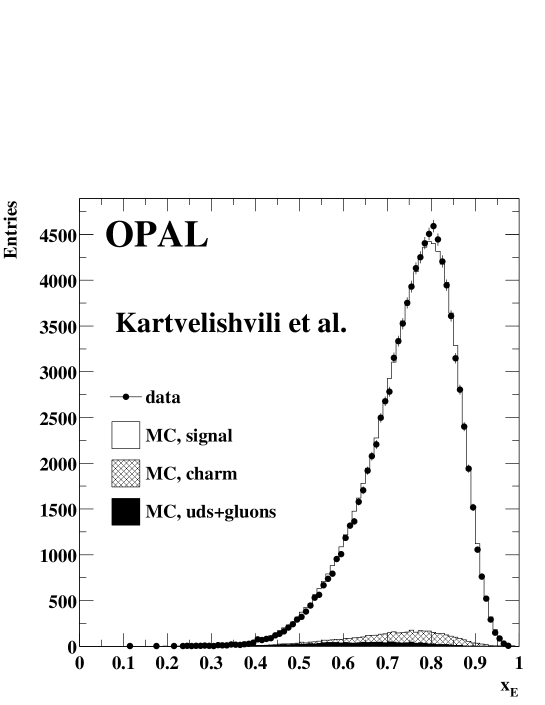
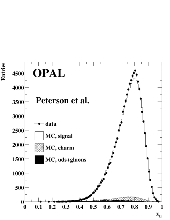
Figure 4: Results of the fit to the data of various hadronisation models for JETSET 7.4. The points with error bars are the uncorrected reconstructed scaled energy distribution in the 1994 data sample. Only statistical errors are shown. The histogram represents the best match as obtained from the respective fragmentation function fits. Background from charm jets is shown as hatched histogram, and light quark and gluon background is indicated by the black area. Charm jets are preferentially passing the selection if the $\mathrm{c}$ quark flight length is large due to a large boost. The mean energy of reconstructed charm candidates is therefore close to that of $\mathrm{b}$ jets.

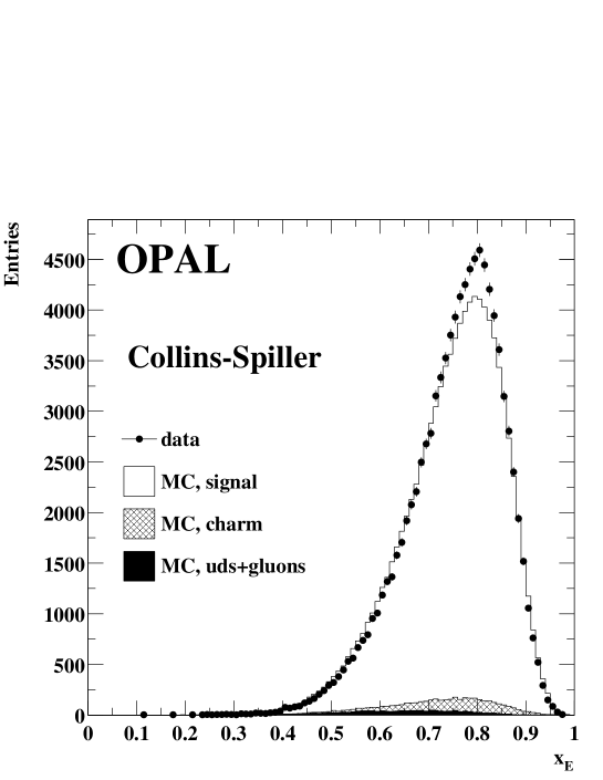
Figure 5: Result of the fit to the data of the Collins-Spiller hadronisation model for JETSET 7.4. The points with error bars are the uncorrected reconstructed scaled energy distribution in the 1994 data sample. Only statistical errors are shown. The histogram represents the best match as obtained from the fragmentation function fit. Background from charm jets is shown as hatched histogram, and light quark and gluon background is indicated by the black area. Charm jets are preferentially passing the selection if the $\mathrm{c}$ quark flight length is large due to a large boost. The mean energy of reconstructed charm candidates is therefore close to that of $\mathrm{b}$ jets.

model	parameters	$\langle\mathit{x}_{\,\mathrm{E}}\rangle$	$\chi^{2}$/d.o.f.
Bowler [26]	$bm_{\perp}^{2}=65.1^{+4.8}_{-3.5}\ {}^{+16.6}_{-13.9}$	$0.7207^{+0.0008}_{-0.0007}\ {}^{+0.0028}_{-0.0029}$	67/44
	$a=0.80^{+0.08}_{-0.06}\ {}^{+0.20}_{-0.21}$
Lund symmetric [27]	$bm_{\perp}^{2}=15.0^{+1.0}_{-0.7}\pm 2.1$	$0.7200^{+0.0009}_{-0.0008}\ {}^{+0.0028}_{-0.0030}$	75/44
	$a=1.59^{+0.13}_{-0.10}\pm 0.27$
Kartvelishvili et al. [25]	$\alpha_{\mathrm{b}}=11.9\pm 0.1\pm 0.5$	$0.7151\pm 0.0006\ ^{+0.0020}_{-0.0023}$	99/45
Peterson et al. [28]	$\varepsilon_{\mathrm{b}}=(41.2\pm 0.7\ ^{+3.6}_{-3.5})\times 10^{-4}$	$0.7023\pm 0.0006\pm 0.0019$	159/45
Collins-Spiller [29]	$\varepsilon_{\mathrm{b}}=(22.3^{+0.7}_{-0.6}\ {}^{+3.5}_{-4.9})\times 10^{-4}$	$0.6870\pm 0.0006\ ^{+0.0035}_{-0.0019}$	407/45
HERWIG 6.2	cldir=1, clsmr(2)=0	0.7074	540/46
HERWIG 5.9	cldir=1, clsmr=0.35	0.6546	4279/46

Table 3: Results of the comparison of hadronisation models to OPAL data. The parameter fit results and corresponding $\mathit{x}_{\,\mathrm{E}}$ values are weighted averages over all datasets from the years 1992–2000, where the weights are chosen according to the subsample size. The first errors on the parameters are statistical, the second systematic. The correlation of the statistical errors of $a$ and $bm_{\perp}^{2}$ is 98.5% for the Lund symmetric model, and 96.4% for the Bowler fragmentation function. The errors on $\langle\mathit{x}_{\,\mathrm{E}}\rangle$ are the propagated statistical parameter errors. The $\chi^{2}$/d.o.f. values are quoted for the 1994 dataset only, which is the largest sample. Only statistical errors are included. The errors of the two parameters of the Lund and Bowler models are almost fully correlated. The parameters given for the HERWIG Monte Carlo are not obtained from a fit, but are the values used for the generation of each sample.

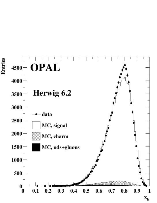
Figure 6: Comparison of different setups of the HERWIG Monte Carlo generator with data. The points with error bars are the uncorrected reconstructed scaled energy distribution in the 1994 data sample. Only statistical errors are shown. The histogram represents the HERWIG prediction. Background from charm jets is shown as hatched histogram, and light quark and gluon background is indicated by the black area.

The reweighting fit is performed separately for each data sample, and the fit results are averaged with weights according to the size of the respective datasets. Consistent results are obtained for all datasets. The average parameter values are summarised in Table 3. For each parametrisation the corresponding model-dependent mean scaled energy of weakly decaying $\mathrm{B}$ hadrons is given. Data samples at $\sqrt{s}=m_{\mathrm{Z}}+1.8\;\mathrm{GeV}$ are excluded in the calculation of the average $\langle\mathit{x}_{\,\mathrm{E}}\rangle$. Table 3 also gives a comparison of the fit quality of all JETSET 7.4 fits on the 1994 data, and the HERWIG 5.9 and HERWIG 6.2 results. The fit results on the 1994 data are shown in Figures 3–6. The ordering of the models according to the goodness of the fits in 1994 data agrees with all other large data samples; only in a few smaller samples is a slightly different ordering observed. The quoted $\chi^{2}$/d.o.f. values only take into account the statistical uncertainty of data and Monte Carlo simulation. Systematic uncertainties are discussed later. The Bowler, Lund symmetric, and Kartvelishvili et al. models are preferred by the data, with respective $\chi^{2}$/d.o.f. values of 67/44, 75/44, and 99/45 in the 1994 sample. Figures 3–6 show that the Peterson et al. and Collins-Spiller parametrisations for JETSET, as well as the HERWIG 6.2 model, are too broad. The HERWIG 5.9 model is too soft.

6 Model-independent measurement of $\langle\mathit{x}_{\,\mathrm{E}}\rangle$

In the previous section, information was extracted from the observed energy distribution making explicit use of a set of models to describe the data. In this section, a measurement of the mean scaled energy of $\mathrm{B}$ hadrons, $\langle\mathit{x}_{\,\mathrm{E}}\rangle$, outside a specific model framework will be presented. This is accomplished by unfolding the observed energy distribution.

Two complementary unfolding procedures are used to obtain an estimate of the true $\mathit{x}_{\,\mathrm{E}}$ distribution from the observed distribution of the reconstructed scaled $\mathrm{B}$ hadron energy. In both cases the amount and energy distribution of background in the $\mathrm{B}$ hadron candidate sample is estimated from the Monte Carlo simulation and subtracted from the data.

The main method starts by fitting the observed data $\mathit{x}_{\,\mathrm{E}}$ distribution, and the observed and the true $\mathit{x}_{\,\mathrm{E}}$ distribution in the Monte Carlo simulation with smooth functions (splines). The true and observed Monte Carlo distributions are then reweighted simultaneously until the observed $\mathit{x}_{\,\mathrm{E}}$ distribution agrees in data and simulation. The reweighted true $\mathit{x}_{\,\mathrm{E}}$ distribution of the Monte Carlo simulation then provides an estimate of the corresponding distribution in data. Details of how the result is stabilised are described later. This method is almost independent of the initial Monte Carlo distribution and thus reduces model-dependence in the unfolding process. Furthermore, the result is represented as an unbinned spline function, which is optimal for the calculation of the mean value of the unfolded distribution. This algorithm is coded using the software package RUN [30] and was already used in [31].

The second approach makes use of the SVD-GURU software package [32]. The correspondence between the observed and true $\mathrm{B}$ hadron energy distributions in the Monte Carlo simulation is represented by a $20\times 20$ matrix. The unfolding process comprises a matrix inversion to obtain an estimate of the true data $\mathit{x}_{\,\mathrm{E}}$ distribution from the observed distribution. In this approach, the model dependence was found to be stronger than when using the RUN program. Furthermore, a coarse binning appropriately adapted to the detector’s resolution and the amount of available data might lead to systematic effects when describing the energy distribution in terms of its mean value. Therefore SVD-GURU is only used to cross-check the result obtained by RUN and to provide an estimate of the systematic uncertainty due to unfolding.

Raw unfolding solutions often oscillate strongly around the correct solution. In the case of a binned representation of the data this effect can simply be understood by strong negative bin-by-bin correlations introduced by the finite detector resolution. Both methods used here suppress these oscillations by limiting the number of degrees of freedom of the unfolding solution. The RUN algorithm represents the unfolding result as expansion into a set of orthogonal functions. The uncertainties on the coefficients of these functions are determined, and only those functions with coefficients significantly different from zero are taken into account. SVD-GURU rotates the unfolding matrix to estimate its effective rank. The unfolding is then performed in a rotated space with a smaller matrix including only the significant contributions. The number of degrees of freedom used for the unfolding procedure was found to agree in the RUN and SVD-GURU approaches in all subsamples described below. A further means of regularisation is available in the RUN package. Of all remaining solutions to the unfolding problem, one is chosen that minimises the integral over the squared first derivative of the unfolding solution. Monte Carlo studies show that this regularisation leads to essentially bias-free results on all samples. The performance of the unfolding algorithms is illustrated in Figure 7.

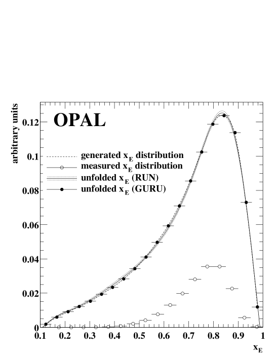
Figure 7: Performance of the unfolding algorithms used in this analysis. The dashed line represents the generated scaled energy distribution of weakly decaying $\mathrm{B}$ hadrons. Open circles with error bars represent the observed $\mathit{x}_{\,\mathrm{E}}$ distribution for Monte Carlo simulated events corresponding to the 1994 OPAL detector setup. Shape and normalisation are different from the generated distribution due to limited and energy-dependent efficiency, detector resolution and reconstruction bias. Full circles with error bars and the solid line with error band indicate the SVD-GURU and RUN unfolding results for this sample.

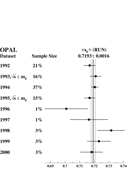
Figure 8: Unfolding results of all data samples with a centre-of-mass energy on or below the $\mathrm{Z}$ mass, obtained with the RUN unfolding package. The fraction of the total data sample contributed by each subsample is given on the left. The vertical line indicates the weighted average $\langle\mathit{x}_{\,\mathrm{E}}\rangle$, and the shaded region represents the uncertainty of this average.

The unfolding is performed separately for data from all years of 1992–2000. The 1993 and 1995 datasets at a centre-of-mass energy below $m_{\mathrm{Z}}$ show $\mathit{x}_{\,\mathrm{E}}$ distributions that are compatible with those taken at the $\mathrm{Z}$ resonance peak in the Monte Carlo simulation. The 1993 and 1995 datasets at $m_{\mathrm{Z}}+1.8\;\mathrm{GeV}$ show a significantly lower $\langle\mathit{x}_{\,\mathrm{E}}\rangle$, caused by a large amount of initial state radiation at this energy. In this case the quark energy prior to fragmentation is lower on average than the beam energy. As the beam energy is used as an estimator of the quark energy prior to fragmentation, the average $\mathit{x}_{\,\mathrm{E}}$ value is lower than in samples without significant initial state radiation. The $m_{\mathrm{Z}}+1.8\;\mathrm{GeV}$ samples are therefore analysed separately.

Both RUN and SVD-GURU analyses are performed with a Monte Carlo simulation that is reweighted to match the best result of the model-dependent reweighting fits for the respective datasets. This procedure is also followed by SLD in their latest $\mathrm{b}$ hadronisation analysis [6]. The goal is to reduce the dependence of the unfolding result on the Monte Carlo sample used for unfolding. The effect of not using the best parametrisation, but the second and third best instead, are studied below as a systematic effect. JETSET 7.4 Monte Carlo simulation samples are used to obtain the central result, and will be compared to unfolding results using HERWIG in the discussion of systematic effects below.

Figure 9: Spline representation of the RUN unfolding result (line with error band), and binned GURU unfolding result (points with error bars), for the full data sample at $\sqrt{s}\leq m_{\mathrm{Z}}$. The narrower error band around the RUN unfolding results corresponds to the statistical uncertainty, the broader error band represents the total uncertainty.

The unfolding result for all data samples at or below the $\mathrm{Z}$ resonance is shown in Figure 8. The mean scaled $\mathrm{B}$ hadron energy, obtained with the RUN unfolding algorithm and averaged over all datasets by using the subsample size for the weights, is

$$\langle\mathit{x}_{\,\mathrm{E}}\rangle=0.7193\pm 0.0016(stat)\ ,$$

where the uncertainty includes the statistical uncertainties due to limited data and Monte Carlo sample sizes, and the statistical uncertainty on the Monte Carlo efficiency. Consistent $\langle\mathit{x}_{\,\mathrm{E}}\rangle$ values were obtained for the individual data samples (see Figure 8). This model-independent measurement agrees with the $\langle\mathit{x}_{\,\mathrm{E}}\rangle$ values in the framework of the best models as seen in Table 3. The unfolding result spline for the full dataset is plotted in Figure 9.

The mean scaled energy observed in the $m_{\mathrm{Z}}+1.8\;\mathrm{GeV}$ samples is found to be

$$\langle\mathit{x}_{\,\mathrm{E}}\rangle=0.7130\pm 0.0056(stat)\ .$$

The 1993 and 1995 $m_{\mathrm{Z}}+1.8\;\mathrm{GeV}$ data samples give consistent values of $\langle\mathit{x}_{\,\mathrm{E}}\rangle$. The difference of the results for the different energies is consistent with the prediction obtained from Monte Carlo samples at similar energies.

The results obtained with the unfolding program SVD-GURU ($0.7195\pm 0.0015(stat)$ for the main dataset, $0.7152\pm 0.0053(stat)$ for the $m_{\mathrm{Z}}+1.8\;\mathrm{GeV}$ samples) are in very good agreement with the ones achieved with the RUN package. This is also demonstrated in Figure 9, where the results obtained from the full $\sqrt{s}\leq m_{\mathrm{Z}}$ data sample by both algorithms are compared. The statistical uncertainties of both methods are also very similar.

7 Systematic uncertainties

Given the large data sample collected with the OPAL detector, and the inclusive character of the analysis presented here, the statistical uncertainties on the results of the previous sections are expected to be small compared to the systematic uncertainties introduced by limited knowledge of physics parameters which possibly affect the measured quantities. In this section, an overview of all systematic checks is given for the reweighting fit and for the unfolding analysis.

The distribution of the $\mathrm{b}$-tagging discriminant in data agrees well with the Monte Carlo simulation. However, it is necessary for this analysis to ensure that this is separately true for different $\mathrm{B}$ hadron energy regions. Therefore the $\mathrm{b}$-tagging discriminant was investigated in ten bins in $\mathit{x}_{\,\mathrm{E}}$. The ratio of the $\mathrm{b}$-tagging discriminant distributions of data and Monte Carlo simulation is calculated and fitted by a linear function in each energy bin separately. The slope of this function is an indicator of the quality of agreement of data and simulation. All fitted slopes are compatible with zero within two standard deviations.

Systematic uncertainties for fits to various models

The systematic checks performed for the fits to models are listed below. The resulting systematic uncertainty estimates for the mean scaled energy $\langle\mathit{x}_{\,\mathrm{E}}\rangle$ in the framework of the respective models are summarised in Table 4.

• The energy resolution of the OPAL calorimeters in the Monte Carlo simulation is varied by $\pm 10\%$ relative to its central value. This range is motivated by jet energy resolution studies in two-jet events, where a difference between the resolution in data and the Monte Carlo simulation of 3.6% was found in some datasets. Under the assumptions that 50% of the total jet energy are contributed by neutral particles and that the observed difference can be fully accounted to the calorimeters, the above variation range covers this effect.

• Similar studies indicate a possible difference of the energy scale between data and simulation of up to 0.4% in some datasets. The energy scale is varied within this range, and the resulting difference of the fit results is taken as systematic uncertainty.

• The resolution of the $r\phi$-related track parameters $d_{0}$ (transverse impact parameter), $\phi_{0}$ (initial azimuth), and $\kappa$ (curvature) is varied in the range $\pm 10\%$ [19].

• The resolution of the $rz$-related track parameters $z_{0}$ (longitudinal impact parameter) and $\tan{\lambda}$ (dip angle, $\lambda=\pi/2-\theta$) is varied by $\pm 10\%$ [19].

• Figure 2a shows a large energy reconstruction bias for low energy $\mathrm{B}$ hadrons. Both the number of low energy $\mathrm{B}$ hadrons and the efficiency for reconstructing them are small. This large bias therefore only affects a very small fraction of the candidates. The effect of possible mismodeling of the bias in the Monte Carlo simulation is evaluated by varying the bias around the values that describe the data best. The reconstruction bias in the high energy region cannot be changed by more than $\pm 1\%$ without leading to a significant degradation of the agreement between data and Monte Carlo simulation. The bias for low energy $\mathrm{B}$ hadrons, with a reconstructed $\mathit{x}_{\,\mathrm{E}}$ below 0.6, is varied by $\pm 10\%$. This range is also motivated by significant degradation of the agreement between data and Monte Carlo simulation. The largest deviations of the measured quantities are taken as systematic uncertainties.

• The relative fraction of different $\mathrm{B}$ hadron species in the sample of primary $\mathrm{B}$ hadrons influences the measurement, because different $\mathrm{B}$ hadron species have different energy distributions. All values obtained in this analysis are calculated with Monte Carlo samples that are reweighted to reflect the current best knowledge of the hadron fractions. The associated systematic uncertainty is estimated by varying the $\mathrm{b}$ baryon fraction within the range $(10.3\pm 1.8)\%$ [33] given by the average of the LEP/SLD/CDF measurements of this quantity. The fraction of $\mathrm{B_{s}}$ in the sample is varied in the range of $(9.8\pm 1.2)\%$ [33].

• The amount of orbitally excited $\mathrm{B}^{(*)}_{\mathit{J}}$ mesons has been measured by all LEP collaborations [21, 34]. An error weighted average of the LEP measurements is $(28.4\pm 3.5)\%$, and the fraction of orbitally excited $\mathrm{B}^{(*)}_{\mathit{J}}$ mesons is varied within this range.

• The Q-value of orbitally excited $\mathrm{B}^{(*)}_{\mathit{J}}$ mesons [24] is about $40\;\mathrm{MeV}$ smaller than the value in the Monte Carlo samples used in this analysis. All results are corrected for this effect, and the difference to the values obtained without correction is taken as systematic uncertainty.

• The average multiplicity of charged particles from a $\mathrm{B}$ hadron decay was found at LEP to be $4.955\pm 0.062$ [33], and is varied within this range.

• The average lifetime of weakly decaying $\mathrm{B}$ hadrons affects the efficiency of secondary vertex reconstruction, and is varied in the range $(1.577\pm 0.016)\;\mathrm{ps}$ [24].

• The average lifetime of weakly decaying charm hadrons determines the amount of charm background found in the $\mathrm{B}$ hadron candidate sample. The $\mathrm{D}^{0}$, $\mathrm{D}^{+}$, $\mathrm{D_{s}}^{+}$, and $\mathrm{\Lambda_{c}}^{+}$ lifetimes are varied within the uncertainties quoted in [24].

• The charm background in the Monte Carlo simulation samples is reweighted to the same hadronisation model as the $\mathrm{B}$ hadron distribution in the respective fits. The central values and uncertainties of the charm fragmentation function are taken from earlier OPAL measurements [35]. For the evaluation of the systematic uncertainty the parameters are varied within their uncertainties.

• Jets from gluon splitting to $\mathrm{b}\overline{\mathrm{b}}$ quark pairs are treated as background in this analysis. To account for the uncertainty of the average LEP result of the gluon splitting rate, $0.00254\pm 0.00050$ $\mathrm{b}\overline{\mathrm{b}}$ pairs per hadronic event [33], the rate is varied within this range.

• The number of $\mathrm{c}\overline{\mathrm{c}}$ pairs from gluon splitting per hadronic event is varied within the LEP uncertainty of $0.0299\pm 0.0039$ [33].

• The partial width of the $\mathrm{Z}$ into $\mathrm{b}\overline{\mathrm{b}}$ quark pairs, normalised to the total hadronic width of the $\mathrm{Z}$, is measured to be $\mathrm{R}_{\mathrm{b}}=0.21646\pm 0.00065$ [24]. Varying this fraction within the quoted uncertainty leads to varying background levels in the unfolding Monte Carlo sample. This causes negligible changes of the fit results.

• The analogous quantity for charm quark pairs, $\mathrm{R}_{\mathrm{c}}$, is less well known, with a current best value of $0.1719\pm 0.0031$ [24]. The impact on the fit results of varying $\mathrm{R}_{\mathrm{c}}$ within this range is negligible.

• Limited knowledge of the LEP beam energy produces a corresponding uncertainty on $\mathit{x}_{\,\mathrm{E}}$, although the dependency of $\mathit{x}_{\,\mathrm{E}}$ on the beam energy is reduced due to the fact that the beam energy also enters the calculation of the reconstructed $\mathrm{B}$ hadron energy via the beam energy constraint. The assumed LEP beam energy is varied within $\pm 8\;\mathrm{MeV}$, which is the largest reported uncertainty for any sample at or close to the $\mathrm{Z}$ resonance [36]. A correlation of 100% between the resulting uncertainties for the different data taking years is assumed.

• The parameter values depend slightly on the $\mathit{x}_{\,\mathrm{E}}$ range used for the fit. The lower end of the fit range is varied within $\mathit{x}_{\,\mathrm{E}}=0.5\pm 0.1$, and the upper range is varied within $\mathit{x}_{\,\mathrm{E}}=0.95\pm 0.05$. The largest deviation from the result obtained using the central values is taken as the systematic uncertainty.

• The bin width used in the fit is varied by $\pm 10\%$. The maximum deviation from the result with standard binning is used to estimate the associated systematic uncertainty.

	Kartvelishvili	Bowler	Lund	Peterson	Collins-Spiller
	et al. [25]	[26]	[27]	et al. [28]	[29]
energy resolution	$\pm 0.0010$	$\pm 0.0015$	$\pm 0.0016$	$\pm 0.0008$	$\pm 0.0010$
energy scale	$\pm 0.0003$	$\pm 0.0004$	${}^{+0.0004}_{-0.0005}$	$\pm 0.0003$	$\pm 0.0003$
$r\phi$ tracking	$\pm 0.0015$	$\pm 0.0021$	$\pm 0.0021$	$\pm 0.0014$	$\pm 0.0013$
$z$ tracking	$\pm 0.0002$	$\pm 0.0003$	$\pm 0.0003$	$\pm 0.0001$	$\pm 0.0001$
bias modeling	$<0.0001$	$\pm 0.0001$	$<0.0001$	$\pm 0.0001$	$\pm 0.0003$
$\mathrm{b}$ baryons	$\pm 0.0002$	${}^{+0.0001}_{-0.0000}$	$<0.0001$	$\pm 0.0002$	$\pm 0.0002$
$\mathrm{B_{s}}$ fraction	$\pm 0.0002$	$\pm 0.0002$	$\pm 0.0002$	${}^{+0.0002}_{-0.0001}$	$\pm 0.0001$
$\mathrm{B}^{(*)}_{\mathit{J}}$ fraction	$\pm 0.0004$	$\pm 0.0001$	$\pm 0.0001$	$\pm 0.0003$	$\pm 0.0003$
$\mathrm{B}^{(*)}_{\mathit{J}}$ Q-value	$<0.0001$	$<0.0001$	$<0.0001$	$<0.0001$	$<0.0001$
$\mathrm{b}$ decay multiplicity	$\pm 0.0002$	$\pm 0.0004$	$\pm 0.0004$	$\pm 0.0002$	$\pm 0.0002$
$\mathrm{b}$ lifetime	$\pm 0.0001$	$\pm 0.0001$	$\pm 0.0001$	$\pm 0.0001$	$\pm 0.0001$
$\mathrm{c}$ lifetime	${}^{+0.0001}_{-0.0002}$	${}^{+0.0001}_{-0.0003}$	${}^{+0.0001}_{-0.0002}$	${}^{+0.0001}_{-0.0002}$	${}^{+0.0001}_{-0.0002}$
charm fragmentation	$\pm 0.0001$	$\pm 0.0001$	$\pm 0.0001$	$\pm 0.0001$	${}^{+0.0000}_{-0.0001}$
$\mathrm{g\to\mathrm{b}\overline{\mathrm{b}}}$ rate	$<0.0001$	$<0.0001$	$\pm 0.0001$	$<0.0001$	$<0.0001$
$\mathrm{g\to\mathrm{c}\overline{\mathrm{c}}}$ rate	$\pm 0.0001$	$\pm 0.0002$	$\pm 0.0002$	$\pm 0.0001$	$\pm 0.0001$
$\mathrm{R}_{\mathrm{b}}$	$<0.0001$	$<0.0001$	$<0.0001$	$<0.0001$	$<0.0001$
$\mathrm{R}_{\mathrm{c}}$	$<0.0001$	$<0.0001$	$<0.0001$	$<0.0001$	$<0.0001$
beam energy	$\pm 0.0001$	$\pm 0.0001$	$\pm 0.0001$	$\pm 0.0001$	$\pm 0.0001$
fit range	${}^{+0.0004}_{-0.0011}$	${}^{+0.0004}_{-0.0009}$	${}^{+0.0005}_{-0.0012}$	${}^{+0.0009}_{-0.0008}$	${}^{+0.0030}_{-0.0008}$
binning effects	$\pm 0.0002$	$\pm 0.0003$	${}^{+0.0003}_{-0.0002}$	$<0.0001$	$<0.0001$
total	${}^{+0.0020}_{-0.0023}$	${}^{+0.0028}_{-0.0029}$	${}^{+0.0028}_{-0.0030}$	$\pm 0.0019$	${}^{+0.0035}_{-0.0019}$

Table 4: Overview of systematic uncertainty contributions to the model-dependent $\langle\mathit{x}_{\,\mathrm{E}}\rangle$ measurements.

The JETSET 7.4 Monte Carlo samples used for the reweighting fit were generated using the Peterson et al. fragmentation function with $\varepsilon_{\mathrm{b}}=38\times 10^{-4}$. The fit result for the Peterson et al. function in data is $\varepsilon_{\mathrm{b}}=(41.2\pm 0.7)\times 10^{-4}$. The fact that the Monte Carlo tuning and the data fit result are close has the advantage that adverse effects due to weights far from 1.0 are not expected. However, additional studies were performed to verify that the closeness of the two values is not introduced by improper reweighting. An older sample of 4 million hadronic JETSET 7.4 events with Peterson et al. fragmentation function with $\varepsilon_{\mathrm{b}}=57\times 10^{-4}$ is used to repeat the fit for the 1994 data sample. The fit result obtained with this sample ($\varepsilon_{\mathrm{b}}=(40.3\pm 1.1)\times 10^{-4}$) is in agreement with the result obtained with the main $\varepsilon_{\mathrm{b}}=38\times 10^{-4}$ 1994 Monte Carlo sample ($\varepsilon_{\mathrm{b}}=(40.6\pm 1.0)\times 10^{-4}$).

Systematic uncertainties of the unfolding analysis

The same systematic uncertainties as for the fragmentation function fits are evaluated also for the $\langle\mathit{x}_{\,\mathrm{E}}\rangle$ measurement, with the exception of fit range effects, which are specific to the model-dependent fit procedure. Binning effects are not present in RUN. The resulting systematic uncertainties are summarised in Table 5.

An additional uncertainty is introduced by the dependence of the $\langle\mathit{x}_{\,\mathrm{E}}\rangle$ measurement on detector and acceptance modelling in the Monte Carlo simulation. As in all unfolding problems, one needs the resolution (or spectral) function $g(x_{0},x)$ where $x_{0}$ is the energy of the hadrons entering the detector and $x$ their measured energy. This function is not measured, but calculated by the OPAL detector simulation [13]. Since the detector simulation is generally made in the framework of some specific Monte-Carlo program generating hadron distributions, a small residual dependency of $g(x_{0},x)$ on the particular Monte Carlo event generator remains. To estimate the associated systematic uncertainty, the unfolding procedure was repeated using not only the best reweighting fit result, but also all other models as initial estimators of the true distribution. This study was performed independently for all datasets. The unfolding was also performed with the JETSET Monte Carlo sample replaced by HERWIG 5.9 and 6.2 samples. The check using JETSET with the Collins-Spiller parametrisation dominates the modelling uncertainty in the negative direction, which is taken as the largest observed deviation from the central $\langle\mathit{x}_{\,\mathrm{E}}\rangle$ value. The uncertainty in the positive direction is dominated by the third best model, which in almost all datasets is the Kartvelishvili et al. parametrisation. The resulting model uncertainty is found to be ${}^{+0.0024}_{-0.0016}$.

The result of the unfolding procedure with the RUN algorithm is cross-checked with the SVD-GURU method, and the difference between the two results is assigned as systematic uncertainty. Furthermore, a difference of similar size is observed between the spline unfolding result of the RUN method and a binned representation of the unfolded distribution. This difference is also included in the unfolding method uncertainty.

	uncertainty contribution
model dependence	${}^{+0.0024}_{-0.0016}$
energy resolution	$\pm 0.0018$
energy scale	$\pm 0.0006$
$r\phi$ tracking	$\pm 0.0013$
$z$ tracking	$\pm 0.0002$
bias modeling	$\pm 0.0011$
$\mathrm{b}$ baryons	$<0.0001$
$\mathrm{B_{s}}$ fraction	$\pm 0.0002$
$\mathrm{B}^{(*)}_{\mathit{J}}$ fraction	$\pm 0.0006$
$\mathrm{B}^{(*)}_{\mathit{J}}$ Q-value	$<0.0001$
$\mathrm{b}$ decay multiplicity	$\pm 0.0006$
$\mathrm{b}$ lifetime	$\pm 0.0007$
$\mathrm{c}$ lifetime	$\pm 0.0001$
charm fragmentation	$\pm 0.0001$
$\mathrm{g\to\mathrm{b}\overline{\mathrm{b}}}$ rate	$\pm 0.0001$
$\mathrm{g\to\mathrm{c}\overline{\mathrm{c}}}$ rate	$\pm 0.0005$
$\mathrm{R}_{\mathrm{b}}$	$<0.0001$
$\mathrm{R}_{\mathrm{c}}$	$<0.0001$
beam energy	$\pm 0.0001$
binning effects	$<0.0001$
unfolding method	$\pm 0.0002$
total	${}^{+0.0038}_{-0.0033}$

Table 5: Summary of all contributions to the total systematic uncertainty of the $\langle\mathit{x}_{\,\mathrm{E}}\rangle$ measurement from the unfolding analysis.

Summing all systematic uncertainties in quadrature yields a total systematic uncertainty on $\langle\mathit{x}_{\,\mathrm{E}}\rangle$ of ${}^{+0.0038}_{-0.0033}$. As expected, the systematic uncertainty is larger than the statistical precision.

Table 6 shows a representation of the RUN result in 20 bins in the $\mathit{x}_{\,\mathrm{E}}$ range between 0.1 and 1.0. This table, along with the full correlation matrix of statistical (Table 7) and systematic (Tables 8 and 9) uncertainties can be used to compare the OPAL results with further hadronisation models not discussed here. It has to be pointed out again that the $\langle\mathit{x}_{\,\mathrm{E}}\rangle$ value obtained from the binned RUN result is smaller than the unbinned result by $\Delta\langle\mathit{x}_{\,\mathrm{E}}\rangle=-0.0002$. This is caused by binning effects which are reduced by using a small bin width, but cannot be entirely avoided.

8 Summary and discussion

Using an unfolding technique to reduce the dependence on $\mathrm{b}$ quark hadronisation models, the mean scaled energy of weakly decaying $\mathrm{B}$ hadrons in $\mathrm{Z}$ decays is measured to be

$$\langle\mathit{x}_{\,\mathrm{E}}\rangle=0.7193\pm 0.0016(stat)^{+0.0038}_{-0.0033}(syst)\ .$$

This is the most precise available measurement of this quantity. Consistent results are obtained using an alternative unfolding method and from model-dependent reweighting fits.

The result obtained here is in good agreement with a recent result from the ALEPH Collaboration [3], $\langle\mathit{x}_{\,\mathrm{E}}\rangle=0.716\pm 0.006(stat)\pm 0.006(syst)$. ALEPH uses exclusive semileptonic $\mathrm{B}$ decays, leading to a smaller candidate sample and thus a larger statistical uncertainty. Another new measurement by SLD [6] gives a somewhat lower value: $\langle\mathit{x}_{\,\mathrm{E}}\rangle=0.709\pm 0.003(stat)\pm 0.003(syst)\pm 0.002(model)$. The difference between the OPAL and the SLD measurements has a statistical significance of less than $2$ standard deviations taking only the uncorrelated uncertainties into account. Another $\langle\mathit{x}_{\,\mathrm{E}}\rangle$ measurement was recently performed using inclusive $\mathrm{B}\to\ell$ decays [5]. Modelling of the lepton energy spectrum introduces additional systematic errors in the lepton-based analysis. The result of $\langle\mathit{x}_{\,\mathrm{E}}\rangle=0.709\pm 0.003(stat)\pm 0.003(syst)\pm 0.013(model)$ is compatible with the analysis presented here, especially given that the result in [5] is not model-independent, but based on a Peterson et al. parametrisation. The LEP average result for $\langle\mathit{x}_{\,\mathrm{E}}\rangle$ in the framework of the Peterson et al. model, obtained from earlier analyses [33], is $0.702\pm 0.008$, again in excellent agreement with the value of $0.7023\pm 0.0006(stat)\pm 0.0019(syst)$ found in this analysis.

The best description of the data with a fragmentation function with one free parameter is achieved with the Kartvelishvili et al. model. The Peterson et al. and Collins-Spiller models produce energy distributions which are too broad to describe the data. Similar features have been observed by SLD and ALEPH in their recent publications. The Bowler and Lund parametrisations, each having two free parameters, achieve a better $\chi^{2}$/d.o.f. in this analysis and are clearly compatible with the data. The same conclusion is reached by SLD while ALEPH did not test these models. The HERWIG cluster model is clearly disfavoured. The main difference of the two HERWIG versions tested in this analysis is the amount of smearing of the $\mathrm{B}$ hadron direction around the initial $\mathrm{b}$ quark direction. Significant smearing is used in the HERWIG 5.9 sample, softening the spectrum too much. The HERWIG 6.2 sample is used without any smearing, giving an $\mathit{x}_{\,\mathrm{E}}$ distribution which is in much better agreement with the data, but which is still too broad. Similar results are obtained by SLD.

The fitted values of the parameters describing each hadronisation model agree less well between the different experiments than the measured $\langle\mathit{x}_{\,\mathrm{E}}\rangle$ values. The parameter values depend critically on details of the Monte Carlo tuning, which is not identical in all respects among the collaborations, although efforts have been made to correct most relevant Monte Carlo parameters to a common set of values.

A general conclusion of the analysis presented here is that the parton shower plus string hadronisation Monte Carlo models provide a good description of the current data. The fragmentation functions derived from intrinsic symmetries of the string model (Bowler, Lund symmetric) are favoured over the phenomenological approaches of Kartvelishvili et al., Peterson et al., and Collins-Spiller.

Acknowledgements

We particularly wish to thank the SL Division for the efficient operation of the LEP accelerator at all energies and for their close cooperation with our experimental group. In addition to the support staff at our own institutions we are pleased to acknowledge the
Department of Energy, USA,
National Science Foundation, USA,
Particle Physics and Astronomy Research Council, UK,
Natural Sciences and Engineering Research Council, Canada,
Israel Science Foundation, administered by the Israel Academy of Science and Humanities,
Benoziyo Center for High Energy Physics,
Japanese Ministry of Education, Culture, Sports, Science and Technology (MEXT) and a grant under the MEXT International Science Research Program,
Japanese Society for the Promotion of Science (JSPS),
German Israeli Bi-national Science Foundation (GIF),
Bundesministerium für Bildung und Forschung, Germany,
National Research Council of Canada,
Hungarian Foundation for Scientific Research, OTKA T-029328, and T-038240,
Fund for Scientific Research, Flanders, F.W.O.-Vlaanderen, Belgium.

bin	$\mathit{x}_{\,\mathrm{E}}$ range	$1/\sigma\ \mathrm{d}\sigma/\mathrm{d}N$
1	0.100–0.145	0.00142 $\pm$ 0.00003  ${}^{+0.00014}_{-0.00011}$
2	0.145–0.190	0.00526 $\pm$ 0.00010  ${}^{+0.00051}_{-0.00044}$
3	0.190–0.235	0.00786 $\pm$ 0.00014  ${}^{+0.00083}_{-0.00061}$
4	0.235–0.280	0.00987 $\pm$ 0.00018  ${}^{+0.00095}_{-0.00045}$
5	0.280–0.325	0.01208 $\pm$ 0.00022  ${}^{+0.00097}_{-0.00044}$
6	0.325–0.370	0.01502 $\pm$ 0.00027  ${}^{+0.00109}_{-0.00076}$
7	0.370–0.415	0.01895 $\pm$ 0.00033  ${}^{+0.00140}_{-0.00079}$
8	0.415–0.460	0.02358 $\pm$ 0.00039  ${}^{+0.00158}_{-0.00080}$
9	0.460–0.505	0.02839 $\pm$ 0.00043  ${}^{+0.00115}_{-0.00129}$
10	0.505–0.550	0.03364 $\pm$ 0.00042  ${}^{+0.00112}_{-0.00269}$
11	0.550–0.595	0.04154 $\pm$ 0.00043  ${}^{+0.00222}_{-0.00380}$
12	0.595–0.640	0.05469 $\pm$ 0.00047  ${}^{+0.00250}_{-0.00340}$
13	0.640–0.685	0.07333 $\pm$ 0.00049  ${}^{+0.00238}_{-0.00250}$
14	0.685–0.730	0.09490 $\pm$ 0.00065  ${}^{+0.00263}_{-0.00220}$
15	0.730–0.775	0.11843 $\pm$ 0.00083  ${}^{+0.00211}_{-0.00212}$
16	0.775–0.820	0.14007 $\pm$ 0.00069  ${}^{+0.00265}_{-0.00860}$
17	0.820–0.865	0.14425 $\pm$ 0.00061  ${}^{+0.00567}_{-0.01376}$
18	0.865–0.910	0.11268 $\pm$ 0.00065  ${}^{+0.00378}_{-0.00560}$
19	0.910–0.955	0.05472 $\pm$ 0.00047  ${}^{+0.00391}_{-0.01055}$
20	0.955–1.000	0.00933 $\pm$ 0.00012  ${}^{+0.00123}_{-0.00322}$

Table 6: Unfolded $\mathit{x}_{\,\mathrm{E}}$ distribution obtained from the RUN program. Statistical and systematic uncertainties are given for each bin. The corresponding correlation matrices are given in Table 7 (statistical uncertainties), Table 8 (positive systematic uncertainties), and Table 9 (negative systematic uncertainties). A binned representation of the RUN result will naturally lead to a slightly different $\langle\mathit{x}_{\,\mathrm{E}}\rangle$ than that calculated from the spline result.

bin	1	2	3	4	5	6	7	8	9	10	11	12	13	14	15	16	17	18	19	20
1	1.00	1.00	1.00	1.00	1.00	1.00	1.00	0.99	0.97	0.91	0.72	0.37	-0.10	-0.48	-0.54	-0.44	-0.02	0.21	0.17	0.08
2		1.00	1.00	1.00	1.00	1.00	1.00	0.99	0.98	0.92	0.71	0.37	-0.10	-0.48	-0.54	-0.44	-0.02	0.21	0.16	0.08
3			1.00	1.00	1.00	1.00	1.00	0.99	0.97	0.91	0.71	0.36	-0.10	-0.48	-0.53	-0.44	-0.02	0.21	0.16	0.08
4				1.00	1.00	1.00	1.00	0.99	0.97	0.91	0.71	0.37	-0.10	-0.48	-0.54	-0.44	-0.02	0.21	0.17	0.08
5					1.00	1.00	1.00	0.99	0.98	0.92	0.72	0.37	-0.09	-0.48	-0.54	-0.44	-0.03	0.21	0.17	0.09
6						1.00	1.00	0.99	0.98	0.92	0.72	0.38	-0.09	-0.48	-0.54	-0.45	-0.03	0.21	0.17	0.08
7							1.00	1.00	0.99	0.93	0.73	0.38	-0.09	-0.48	-0.54	-0.44	-0.02	0.20	0.16	0.07
8								1.00	0.99	0.94	0.75	0.40	-0.08	-0.47	-0.54	-0.45	-0.03	0.20	0.15	0.07
9									1.00	0.97	0.81	0.48	-0.00	-0.45	-0.56	-0.49	-0.06	0.20	0.17	0.08
10										1.00	0.92	0.67	0.19	-0.39	-0.60	-0.60	-0.15	0.19	0.22	0.15
11											1.00	0.90	0.49	-0.20	-0.57	-0.69	-0.30	0.13	0.26	0.25
12												1.00	0.80	0.14	-0.33	-0.60	-0.46	-0.05	0.18	0.26
13													1.00	0.69	0.26	-0.18	-0.57	-0.43	-0.13	0.06
14														1.00	0.87	0.49	-0.37	-0.69	-0.51	-0.28
15															1.00	0.83	-0.02	-0.58	-0.61	-0.46
16																1.00	0.52	-0.16	-0.46	-0.51
17																	1.00	0.72	0.26	-0.05
18																		1.00	0.83	0.57
19																			1.00	0.93
20																				1.00

Table 7: Correlation matrix of statistical uncertainties of the distribution in Table 6.

bin	1	2	3	4	5	6	7	8	9	10	11	12	13	14	15	16	17	18	19	20
1	1.00	1.00	1.00	1.00	0.99	0.99	0.99	0.98	0.89	-0.28	-0.69	-0.67	-0.50	-0.51	-0.65	0.17	0.44	0.18	-0.94	-0.74
2		1.00	1.00	1.00	1.00	0.99	0.99	0.99	0.90	-0.28	-0.69	-0.67	-0.51	-0.52	-0.66	0.17	0.44	0.18	-0.94	-0.74
3			1.00	1.00	0.99	0.99	0.99	0.98	0.88	-0.32	-0.72	-0.70	-0.54	-0.56	-0.67	0.21	0.48	0.23	-0.95	-0.77
4				1.00	1.00	0.99	0.99	0.99	0.89	-0.29	-0.70	-0.68	-0.53	-0.55	-0.68	0.18	0.46	0.21	-0.94	-0.76
5					1.00	1.00	1.00	1.00	0.92	-0.22	-0.64	-0.63	-0.48	-0.52	-0.68	0.11	0.40	0.15	-0.92	-0.71
6						1.00	1.00	1.00	0.94	-0.17	-0.61	-0.60	-0.45	-0.50	-0.69	0.06	0.37	0.13	-0.90	-0.69
7							1.00	1.00	0.93	-0.19	-0.63	-0.62	-0.48	-0.53	-0.71	0.09	0.40	0.16	-0.91	-0.71
8								1.00	0.95	-0.16	-0.60	-0.59	-0.46	-0.52	-0.72	0.05	0.38	0.14	-0.89	-0.69
9									1.00	0.17	-0.31	-0.31	-0.20	-0.34	-0.68	-0.27	0.09	-0.11	-0.71	-0.44
10										1.00	0.88	0.86	0.78	0.57	0.13	-0.98	-0.88	-0.77	0.54	0.77
11											1.00	0.99	0.87	0.74	0.47	-0.82	-0.91	-0.72	0.86	0.96
12												1.00	0.94	0.83	0.57	-0.83	-0.95	-0.80	0.82	0.98
13													1.00	0.95	0.69	-0.80	-0.98	-0.93	0.62	0.92
14														1.00	0.86	-0.60	-0.89	-0.89	0.56	0.85
15															1.00	-0.13	-0.56	-0.55	0.54	0.66
16																1.00	0.89	0.83	-0.44	-0.74
17																	1.00	0.94	-0.62	-0.92
18																		1.00	-0.34	-0.75
19																			1.00	0.87
20																				1.00

Table 8: Correlation matrix of positive systematic uncertainties of the distribution in Table 6.

bin	1	2	3	4	5	6	7	8	9	10	11	12	13	14	15	16	17	18	19	20
1	1.00	0.99	0.99	0.94	-0.00	-0.40	-0.28	-0.10	-0.44	-0.70	-0.75	-0.69	-0.45	-0.24	0.58	0.75	0.73	0.49	-0.90	-0.82
2		1.00	1.00	0.93	-0.06	-0.45	-0.34	-0.16	-0.49	-0.74	-0.79	-0.73	-0.50	-0.28	0.59	0.79	0.77	0.54	-0.92	-0.86
3			1.00	0.93	-0.05	-0.45	-0.33	-0.15	-0.48	-0.74	-0.79	-0.73	-0.51	-0.30	0.58	0.78	0.77	0.54	-0.92	-0.86
4				1.00	0.31	-0.10	0.03	0.21	-0.15	-0.45	-0.52	-0.46	-0.24	-0.11	0.39	0.52	0.51	0.25	-0.72	-0.62
5					1.00	0.92	0.96	0.98	0.88	0.70	0.64	0.67	0.70	0.51	-0.45	-0.65	-0.65	-0.76	0.43	0.54
6						1.00	0.99	0.94	0.98	0.92	0.89	0.89	0.83	0.56	-0.64	-0.89	-0.89	-0.89	0.76	0.83
7							1.00	0.98	0.98	0.87	0.83	0.84	0.79	0.53	-0.63	-0.83	-0.82	-0.85	0.67	0.75
8								1.00	0.94	0.77	0.72	0.74	0.73	0.47	-0.57	-0.72	-0.70	-0.78	0.52	0.61
9									1.00	0.95	0.92	0.92	0.84	0.55	-0.70	-0.92	-0.90	-0.89	0.78	0.84
10										1.00	1.00	0.99	0.85	0.55	-0.74	-1.00	-0.98	-0.90	0.94	0.97
11											1.00	0.99	0.85	0.57	-0.72	-1.00	-0.99	-0.89	0.96	0.98
12												1.00	0.92	0.66	-0.64	-0.99	-0.99	-0.94	0.92	0.97
13													1.00	0.89	-0.30	-0.85	-0.90	-0.99	0.71	0.83
14														1.00	0.15	-0.57	-0.67	-0.86	0.44	0.59
15															1.00	0.71	0.61	0.38	-0.72	-0.65
16																1.00	0.99	0.90	-0.96	-0.99
17																	1.00	0.94	-0.94	-0.99
18																		1.00	-0.77	-0.88
19																			1.00	0.98
20																				1.00

Table 9: Correlation matrix of negative systematic uncertainties of the distribution in Table 6.

References

-
[1]
Ya.I. Azimov, L.L. Frankfurt, V.A. Khoze,
Leningrad preprint LNPI-222, 1976,
in Proceedings of XVIII Int. Conf. on High Energy Physics (Tbilisi, 1976),
Dubna, II, B10, 1977;
J.D. Bjorken, Phys. Rev. D17 (1978) 171. -
[2]
ALEPH Collaboration, D. Buskulic et al.,
Phys. Lett. B357 (1995) 699;
OPAL Collaboration, G. Alexander et al., Phys. Lett. B364 (1995) 93. - [3] ALEPH Collaboration, A. Heister et al., Phys. Lett. B512 (2001) 30.
-
[4]
ALEPH Collaboration, D. Buskulic et al.,
Z. Phys. C62 (1994) 179;
DELPHI Collaboration, P. Abreu et al., Z. Phys. C66 (1995) 323;
OPAL Collaboration, R. Akers et al., Z. Phys. C60 (1993) 199. - [5] OPAL Collaboration, G. Abbiendi et al., Eur. Phys. J. C13 (2000) 225.
- [6] SLD Collaboration, K. Abe et al., Phys. Rev. D65 (2002) 092006.
-
[7]
OPAL Collaboration, K. Ahmet et al.,
Nucl. Instr. Meth. A305 (1991) 275;
OPAL Collaboration, P.P. Allport et al., Nucl. Instr. Meth. A324 (1993) 34;
M. Hauschild et al., Nucl. Instr. Meth. A314 (1992) 74;
O. Biebel et al., Nucl. Instr. Meth. A323 (1992) 169. - [8] OPAL Collaboration, G. Abbiendi et al., Z. Phys. C74 (1997) 1.
- [9] T. Sjöstrand, Comp. Phys. Comm. 82 (1994) 74.
- [10] G. Marchesini et al., Comp. Phys. Comm. 67 (1992) 465.
- [11] G. Corcella et al., JHEP 0101 (2001) 010.
-
[12]
Jetset 7.4 and Herwig 5.8/5.9:
OPAL Collaboration, G. Alexander et al., Z. Phys. C69 (1996) 543;
Herwig 6.2:
OPAL Collaboration, G. Alexander et al., Phys. Lett. B539 (2002) 13. - [13] J. Allison et al., Nucl. Instr. Meth. A317 (1991) 47.
-
[14]
OPAL Collaboration, P.P. Allport et al.,
Nucl. Instr. Meth. A346 (1994) 476;
OPAL Collaboration, S. Anderson et al., Nucl. Instr. Meth. A403 (1998) 326. -
[15]
N. Brown, W.J. Stirling, Phys. Lett. B252 (1990) 657;
S. Bethke, Z. Kunszt, D. Soper, W.J. Stirling, Nucl. Phys. B370 (1992) 310;
S. Catani et al., Phys. Lett. B269 (1991) 432;
N. Brown, W.J. Stirling, Z. Phys. C53 (1992) 629. - [16] OPAL Collaboration, K. Ackerstaff et al., Eur. Phys. J. C2 (1998) 213.
- [17] OPAL Collaboration, G. Abbiendi et al., Eur. Phys. J. C7 (1999) 407.
- [18] OPAL Collaboration, G. Abbiendi et al., Eur. Phys. J. C23 (2002) 397.
- [19] OPAL Collaboration, G. Abbiendi et al., Eur. Phys. J. C8 (1999) 217.
- [20] OPAL Collaboration, R. Akers et al., Z. Phys. C63 (1994) 197.
- [21] OPAL Collaboration, G. Alexander et al., Z. Phys. C66 (1995) 19.
- [22] OPAL Collaboration, G. Abbiendi et al., Eur. Phys. J. C23 (2002) 437.
-
[23]
The neural networks were trained using JETNET 3:
C. Peterson, T. Rögnvaldsson and L. Lönnblad, Comp. Phys. Comm. 81 (1994) 185. - [24] Particle Data Group, D.E. Groom et al., Eur. Phys. J. C15 (2000) 1.
- [25] V.G. Kartvelishvili, A.K. Likhoded, V.A. Petrov, Phys. Lett. B78 (1978) 615.
- [26] M.G. Bowler, Z. Phys. C11 (1981) 169.
- [27] B. Andersson, G. Gustafson, B. Söderberg, Z. Phys. C20 (1983) 317.
- [28] C. Peterson, D. Schlatter, I. Schmitt, P.M. Zerwas, Phys. Rev. D27 (1983) 105.
- [29] P.D.B. Collins, T.P. Spiller, J. Phys. G11 (1985) 1289.
- [30] V. Blobel, Unfolding Methods for High-Energy Physics Experiments, in Proceedings of CERN Computing School, 1984 (Aiguablava, Spain, 1984), CERN Yellow Report CERN 85-09, C. Verkerk (Ed.), p. 88, and DESY 84-118 (1984)
- [31] OPAL Collaboration, G. Abbiendi et al., Eur. Phys. J. C18 (2000) 15.
- [32] A. Hocker, V. Kartvelishvili, Nucl. Instr. Meth. A372 (1996) 469.
- [33] ALEPH, CDF, DELPHI, L3, OPAL, and SLD Collaborations, Combined Results on b-Hadron Production Rates and Decay Properties, CERN-EP/2001-050.
-
[34]
DELPHI Collaboration,
P. Abreu et al., Phys. Lett. B345 (1995) 598;
ALEPH Collaboration, R. Barate et al., Phys. Lett. B425 (1998) 215;
L3 Collaboration, M. Acciarri et al., Phys. Lett. B465 (1999) 323. - [35] OPAL Collaboration, K. Ackerstaff et al., Eur. Phys. J. C1 (1998) 439.
-
[36]
LEP Energy Working Group, R. Assmann et al.,
Phys. Lett. B307 (1993) 187;
LEP Energy Working Group, R. Assmann et al., Eur. Phys. J. C6 (1999) 187.