EUROPEAN ORGANIZATION FOR NUCLEAR RESEARCH

CERN-EP/2002-053

July 12, 2002

Measurement of the b quark forward-backward asymmetry around the $\rm Z^{0}$ peak using an inclusive tag

The OPAL collaboration

The b quark forward-backward asymmetry has been measured using hadronic $\rm Z^{0}$ decays collected by the OPAL experiment at LEP. $\rm\mbox{$\rm Z^{0}$}\rightarrow\mbox{$\rm b\overline{b}$}$ decays were selected using a combination of secondary vertex and lepton tags, and the sign of the b quark charge was determined using an inclusive tag based on jet, vertex and kaon charges. The results, corrected to the quark level, are:

$A^{\rm b}_{\rm FB}$	=	$0.0582\pm 0.0153\pm 0.0012$	at  $\sqrt{s}=89.50$ GeV
$A^{\rm b}_{\rm FB}$	=	$0.0977\pm 0.0036\pm 0.0018$	at  $\sqrt{s}=91.26$ GeV
$A^{\rm b}_{\rm FB}$	=	$0.1221\pm 0.0123\pm 0.0025$	at  $\sqrt{s}=92.91$ GeV

where the first error is statistical and the second systematic in each case. Within the framework of the Standard Model, the result is interpreted as a measurement of the effective weak mixing angle for electrons of $\mbox{$\rm\sin^{2}\theta_{W}^{eff,e}$}=0.23205\pm 0.00068$.

Submitted to Physics Letters B.

The OPAL Collaboration

G. Abbiendi², C. Ainsley⁵, P.F. Åkesson³, G. Alexander²², J. Allison¹⁶, P. Amaral⁹, G. Anagnostou¹, K.J. Anderson⁹, S. Arcelli², S. Asai²³, D. Axen²⁷, G. Azuelos^18,a, I. Bailey²⁶, E. Barberio⁸, R.J. Barlow¹⁶, R.J. Batley⁵, P. Bechtle²⁵, T. Behnke²⁵, K.W. Bell²⁰, P.J. Bell¹, G. Bella²², A. Bellerive⁶, G. Benelli⁴, S. Bethke³², O. Biebel³¹, I.J. Bloodworth¹, O. Boeriu¹⁰, P. Bock¹¹, D. Bonacorsi², M. Boutemeur³¹, S. Braibant⁸, L. Brigliadori², R.M. Brown²⁰, K. Buesser²⁵, H.J. Burckhart⁸, S. Campana⁴, R.K. Carnegie⁶, B. Caron²⁸, A.A. Carter¹³, J.R. Carter⁵, C.Y. Chang¹⁷, D.G. Charlton^1,b, A. Csilling^8,g, M. Cuffiani², S. Dado²¹, G.M. Dallavalle², S. Dallison¹⁶, A. De Roeck⁸, E.A. De Wolf⁸, K. Desch²⁵, B. Dienes³⁰, M. Donkers⁶, J. Dubbert³¹, E. Duchovni²⁴, G. Duckeck³¹, I.P. Duerdoth¹⁶, E. Elfgren¹⁸, E. Etzion²², F. Fabbri², L. Feld¹⁰, P. Ferrari⁸, F. Fiedler³¹, I. Fleck¹⁰, M. Ford⁵, A. Frey⁸, A. Fürtjes⁸, P. Gagnon¹², J.W. Gary⁴, G. Gaycken²⁵, C. Geich-Gimbel³, G. Giacomelli², P. Giacomelli², M. Giunta⁴, J. Goldberg²¹, E. Gross²⁴, J. Grunhaus²², M. Gruwé⁸, P.O. Günther³, A. Gupta⁹, C. Hajdu²⁹, M. Hamann²⁵, G.G. Hanson⁴, K. Harder²⁵, A. Harel²¹, M. Harin-Dirac⁴, M. Hauschild⁸, J. Hauschildt²⁵, C.M. Hawkes¹, R. Hawkings⁸, R.J. Hemingway⁶, C. Hensel²⁵, G. Herten¹⁰, R.D. Heuer²⁵, J.C. Hill⁵, K. Hoffman⁹, R.J. Homer¹, D. Horváth^29,c, R. Howard²⁷, P. Hüntemeyer²⁵, P. Igo-Kemenes¹¹, K. Ishii²³, H. Jeremie¹⁸, P. Jovanovic¹, T.R. Junk⁶, N. Kanaya²⁶, J. Kanzaki²³, G. Karapetian¹⁸, D. Karlen⁶, V. Kartvelishvili¹⁶, K. Kawagoe²³, T. Kawamoto²³, R.K. Keeler²⁶, R.G. Kellogg¹⁷, B.W. Kennedy²⁰, D.H. Kim¹⁹, K. Klein¹¹, A. Klier²⁴, S. Kluth³², T. Kobayashi²³, M. Kobel³, S. Komamiya²³, L. Kormos²⁶, R.V. Kowalewski²⁶, T. Krämer²⁵, T. Kress⁴, P. Krieger^6,l, J. von Krogh¹¹, D. Krop¹², K. Kruger⁸, M. Kupper²⁴, G.D. Lafferty¹⁶, H. Landsman²¹, D. Lanske¹⁴, J.G. Layter⁴, A. Leins³¹, D. Lellouch²⁴, J. Letts¹², L. Levinson²⁴, J. Lillich¹⁰, S.L. Lloyd¹³, F.K. Loebinger¹⁶, J. Lu²⁷, J. Ludwig¹⁰, A. Macpherson^28,i, W. Mader³, S. Marcellini², T.E. Marchant¹⁶, A.J. Martin¹³, J.P. Martin¹⁸, G. Masetti², T. Mashimo²³, P. Mättig^m, W.J. McDonald²⁸, J. McKenna²⁷, T.J. McMahon¹, R.A. McPherson²⁶, F. Meijers⁸, P. Mendez-Lorenzo³¹, W. Menges²⁵, F.S. Merritt⁹, H. Mes^6,a, A. Michelini², S. Mihara²³, G. Mikenberg²⁴, D.J. Miller¹⁵, S. Moed²¹, W. Mohr¹⁰, T. Mori²³, A. Mutter¹⁰, K. Nagai¹³, I. Nakamura²³, H.A. Neal³³, R. Nisius³², S.W. O’Neale¹, A. Oh⁸, A. Okpara¹¹, M.J. Oreglia⁹, S. Orito²³, C. Pahl³², G. Pásztor^4,g, J.R. Pater¹⁶, G.N. Patrick²⁰, J.E. Pilcher⁹, J. Pinfold²⁸, D.E. Plane⁸, B. Poli², J. Polok⁸, O. Pooth¹⁴, M. Przybycień^8,n, A. Quadt³, K. Rabbertz⁸, C. Rembser⁸, P. Renkel²⁴, H. Rick⁴, J.M. Roney²⁶, S. Rosati³, Y. Rozen²¹, K. Runge¹⁰, K. Sachs⁶, T. Saeki²³, O. Sahr³¹, E.K.G. Sarkisyan^8,j, A.D. Schaile³¹, O. Schaile³¹, P. Scharff-Hansen⁸, J. Schieck³², T. Schörner-Sadenius⁸, M. Schröder⁸, M. Schumacher³, C. Schwick⁸, W.G. Scott²⁰, R. Seuster^14,f, T.G. Shears^8,h, B.C. Shen⁴, C.H. Shepherd-Themistocleous⁵, P. Sherwood¹⁵, G. Siroli², A. Skuja¹⁷, A.M. Smith⁸, R. Sobie²⁶, S. Söldner-Rembold^10,d, S. Spagnolo²⁰, F. Spano⁹, A. Stahl³, K. Stephens¹⁶, D. Strom¹⁹, R. Ströhmer³¹, S. Tarem²¹, M. Tasevsky⁸, R.J. Taylor¹⁵, R. Teuscher⁹, M.A. Thomson⁵, E. Torrence¹⁹, D. Toya²³, P. Tran⁴, T. Trefzger³¹, A. Tricoli², I. Trigger⁸, Z. Trócsányi^30,e, E. Tsur²², M.F. Turner-Watson¹, I. Ueda²³, B. Ujvári^30,e, B. Vachon²⁶, C.F. Vollmer³¹, P. Vannerem¹⁰, M. Verzocchi¹⁷, H. Voss⁸, J. Vossebeld^8,h, D. Waller⁶, C.P. Ward⁵, D.R. Ward⁵, P.M. Watkins¹, A.T. Watson¹, N.K. Watson¹, P.S. Wells⁸, T. Wengler⁸, N. Wermes³, D. Wetterling¹¹ G.W. Wilson^16,k, J.A. Wilson¹, G. Wolf²⁴, T.R. Wyatt¹⁶, S. Yamashita²³, D. Zer-Zion⁴, L. Zivkovic²⁴

¹School of Physics and Astronomy, University of Birmingham, Birmingham B15 2TT, UK
²Dipartimento di Fisica dell’ Università di Bologna and INFN, I-40126 Bologna, Italy
³Physikalisches Institut, Universität Bonn, D-53115 Bonn, Germany
⁴Department of Physics, University of California, Riverside CA 92521, USA
⁵Cavendish Laboratory, Cambridge CB3 0HE, UK
⁶Ottawa-Carleton Institute for Physics, Department of Physics, Carleton University, Ottawa, Ontario K1S 5B6, Canada
⁸CERN, European Organisation for Nuclear Research, CH-1211 Geneva 23, Switzerland
⁹Enrico Fermi Institute and Department of Physics, University of Chicago, Chicago IL 60637, USA
¹⁰Fakultät für Physik, Albert-Ludwigs-Universität Freiburg, D-79104 Freiburg, Germany
¹¹Physikalisches Institut, Universität Heidelberg, D-69120 Heidelberg, Germany
¹²Indiana University, Department of Physics, Swain Hall West 117, Bloomington IN 47405, USA
¹³Queen Mary and Westfield College, University of London, London E1 4NS, UK
¹⁴Technische Hochschule Aachen, III Physikalisches Institut, Sommerfeldstrasse 26-28, D-52056 Aachen, Germany
¹⁵University College London, London WC1E 6BT, UK
¹⁶Department of Physics, Schuster Laboratory, The University, Manchester M13 9PL, UK
¹⁷Department of Physics, University of Maryland, College Park, MD 20742, USA
¹⁸Laboratoire de Physique Nucléaire, Université de Montréal, Montréal, Quebec H3C 3J7, Canada
¹⁹University of Oregon, Department of Physics, Eugene OR 97403, USA
²⁰CLRC Rutherford Appleton Laboratory, Chilton, Didcot, Oxfordshire OX11 0QX, UK
²¹Department of Physics, Technion-Israel Institute of Technology, Haifa 32000, Israel
²²Department of Physics and Astronomy, Tel Aviv University, Tel Aviv 69978, Israel
²³International Centre for Elementary Particle Physics and Department of Physics, University of Tokyo, Tokyo 113-0033, and Kobe University, Kobe 657-8501, Japan
²⁴Particle Physics Department, Weizmann Institute of Science, Rehovot 76100, Israel
²⁵Universität Hamburg/DESY, Institut für Experimentalphysik, Notkestrasse 85, D-22607 Hamburg, Germany
²⁶University of Victoria, Department of Physics, P O Box 3055, Victoria BC V8W 3P6, Canada
²⁷University of British Columbia, Department of Physics, Vancouver BC V6T 1Z1, Canada
²⁸University of Alberta, Department of Physics, Edmonton AB T6G 2J1, Canada
²⁹Research Institute for Particle and Nuclear Physics, H-1525 Budapest, P O Box 49, Hungary
³⁰Institute of Nuclear Research, H-4001 Debrecen, P O Box 51, Hungary
³¹Ludwig-Maximilians-Universität München, Sektion Physik, Am Coulombwall 1, D-85748 Garching, Germany
³²Max-Planck-Institute für Physik, Föhringer Ring 6, D-80805 München, Germany
³³Yale University, Department of Physics, New Haven, CT 06520, USA

^a and at TRIUMF, Vancouver, Canada V6T 2A3
^b and Royal Society University Research Fellow
^c and Institute of Nuclear Research, Debrecen, Hungary
^d and Heisenberg Fellow
^e and Department of Experimental Physics, Lajos Kossuth University, Debrecen, Hungary
^f and MPI München
^g and Research Institute for Particle and Nuclear Physics, Budapest, Hungary
^h now at University of Liverpool, Dept of Physics, Liverpool L69 3BX, UK
ⁱ and CERN, EP Div, 1211 Geneva 23
^j and Universitaire Instelling Antwerpen, Physics Department, B-2610 Antwerpen, Belgium
^k now at University of Kansas, Dept of Physics and Astronomy, Lawrence, KS 66045, USA
^l now at University of Toronto, Dept of Physics, Toronto, Canada
^m current address Bergische Universität, Wuppertal, Germany
ⁿ and University of Mining and Metallurgy, Cracow, Poland

1 Introduction

The measurement of $A^{\rm b}_{\rm FB}$, the forward-backward asymmetry of b quarks produced in $\mbox{$\rm e^{+}e^{-}$}\rightarrow\mbox{$\rm b\overline{b}$}$ events, provides an important test of the Standard Model, allowing the effective weak mixing angle $\rm\sin^{2}\theta_{W}^{eff}$ to be determined with high precision [1]. The differential cross-section for the production of $\rm b\overline{b}$ pairs can be written as

$$\frac{{\rm d}\sigma}{{\rm d}\cos\theta}\propto 1+\cos^{2}\theta+\frac{8}{3}\mbox{$A^{\rm b}_{\rm FB}$}\cos\theta\,,$$

where $\theta$ is the angle between the directions of the incoming electron and outgoing b quark, and where initial and final state radiation, quark mass and higher order terms have been neglected. The Standard Model prediction of the $\rm Z^{0}$ pole asymmetry $A^{\rm b,0}_{\rm FB}$ can be written

$$\mbox{$A^{\rm b,0}_{\rm FB}$}=\frac{3}{4}\left(\frac{2g^{\rm e}_{V}g^{\rm e}_{A}}{(g^{\rm e}_{V})^{2}+(g^{\rm e}_{A})^{2}}\right)\left(\frac{2g^{\rm b}_{V}g^{\rm b}_{A}}{(g^{\rm b}_{V})^{2}+(g^{\rm b}_{A})^{2}}\right)\,,$$

where $g_{V}^{\rm e,b}$ and $g_{A}^{\rm e,b}$ are the effective vector and axial-vector couplings of the electron and b quark to the $\rm Z^{0}$. The effective weak mixing angle $\rm\sin^{2}\theta_{W}^{eff,f}$ for a charged fermion f can be expressed as

$$\mbox{$\rm\sin^{2}\theta_{W}^{eff,f}$}=\frac{1}{4|q_{\rm f}|}\left(1-\frac{g^{\rm f}_{V}}{g^{\rm f}_{A}}\right)\,,$$

where $q_{\rm f}$ is the electric charge of the fermion in units of the electron charge. With the values of the electron and b quark couplings predicted in the Standard Model, the asymmetry $A^{\rm b,0}_{\rm FB}$ is mainly sensitive to the weak mixing angle for electrons, $\rm\sin^{2}\theta_{W}^{eff,e}$, and insensitive to that for b quarks. The weak mixing angle $\rm\sin^{2}\theta_{W}^{eff,e}$ can therefore be determined from the measured asymmetry within the context of the Standard Model, which also predicts the centre-of-mass energy dependence of the asymmetry arising from $\rm Z^{0}$-$\gamma$ interference [1].

The most sensitive measurements of $\rm\sin^{2}\theta_{W}^{eff,e}$ at LEP come from the measurements of the b quark asymmetry, using techniques based on jet charges, secondary vertices and high momentum leptons [2, 3, 4]. This paper reports an improved measurement of $A^{\rm b}_{\rm FB}$ using jet, vertex and kaon charges combined in an inclusive tag. Compared to the previous OPAL analysis using jet and vertex charges [3], the measurement is improved by using the high-performance b-tagging technique developed for the measurement of $R_{\rm b}$ [5] incorporating both vertex- and lepton-based b-tags, b quark charge tagging methods developed for $\rm B^{0}$ oscillation and CP-violation measurements [6, 7, 8], an increased angular acceptance and a more sophisticated fitting technique measuring more of the required event properties from the data themselves. The data sample is also increased by adding about 0.5 million $\rm Z^{0}$ decays recorded primarily for calibration purposes during the LEP2 physics programme between 1996 and 2000.

A brief outline of the analysis method is given in the following section, followed by a description of the data sample, the $\rm b\overline{b}$ event tagging and the b quark charge tagging in sections 3 to 5. The fit method and results are described in section 6, and a discussion of systematic uncertainties is given in section 7. A summary of the asymmetry results and interpretation in terms of $\rm\sin^{2}\theta_{W}^{eff,e}$ are given in section 8.

2 Analysis method

The analysis method exploits the structure of $\mbox{$\rm Z^{0}$}\rightarrow\mbox{$\rm b\overline{b}$}$ events, which tend to be composed of two back-to-back jets, each containing the decay products of one of the b quarks. Each event was divided into two hemispheres by the plane perpendicular to the thrust axis and containing the interaction point, and the two hemispheres, each typically containing one b jet, were considered independently. The direction of the thrust axis, in particular its polar angle $\theta_{T}$, was used as an estimate of the original b quark direction. The hemisphere containing the positive $z$-axis, i.e. the outgoing electron beam direction, was labelled ‘forward’, and the other hemisphere labelled ‘backward’. Two b-tagging algorithms, based on secondary vertices and high momentum leptons, were applied to each hemisphere, and used to define four classes of b-tagged hemispheres of differing purity (see section 4). The numbers of events with b-tags in one or both hemispheres, together with externally-input values of $R_{\rm b}$ and $R_{\rm c}$ (the fraction of hadronic $\rm Z^{0}$ decays to $\rm b\overline{b}$ and $\rm c\overline{c}$) provide enough information to determine the b and c quark tagging efficiencies for each tag with only small dependence on Monte Carlo simulation. Jet, vertex and kaon charge information in each hemisphere was then used to determine the production flavour of the b hadron in the hemisphere, and hence the sign of the underlying quark charge (b or $\rm\overline{b}$—see section 5). The two hemisphere determinations were combined to produce a better estimate for the whole event. Since each event contains a b and a $\rm\overline{b}$ quark, the fraction of events where the two tags agree can be used to produce an estimate of the reliability (mistag fraction) of the production flavour tag. The asymmetry $A^{\rm b}_{\rm FB}$ was then extracted from the production flavour tag distributions in forward and backward hemispheres, for five bins in $|\mbox{$\cos\theta_{T}$}|$ and 14 event classes with different combinations of b-tags in each hemisphere.

In this method, the most important quantities needed for the analysis, i.e. the b- and c-tagging efficiencies and the fraction of hemispheres with an incorrect production flavour tag, are extracted directly from the data as a function of $|\mbox{$\cos\theta_{T}$}|$. Monte Carlo simulation is needed to determine the tagging efficiencies and mistag fractions for light quark events, the mistag fraction for charm events, and the effects of correlations between the two hemispheres in $\rm b\overline{b}$ events, which result in small corrections to both the b efficiencies and mistag fractions. The uncertainties in all these input quantities result in systematic errors that are much smaller than the data statistical error.

3 Data sample and event simulation

The OPAL detector is well described elsewhere [9, 10, 11]. This analysis relies mainly on charged particle track reconstruction using the central tracking chambers and the silicon microvertex detector. The latter was first operational in 1991, providing measurements in the $r$-$\phi$ plane only. In 1993 it was upgraded to measure tracks in both $r$-$\phi$ and $r$-$z$ planes [10], and in 1996 the $\cos\theta$ coverage for at least one silicon measurement was extended from $|\cos\theta|<0.83$ to $|\cos\theta|<0.93$ [11]. To account for the changing detector performance with time, the analysis was performed separately for data taken in 1991–1992, 1993, 1994, 1995 and 1996–2000, and the results were finally combined.

Hadronic $\rm Z^{0}$ decays were selected using standard criteria, as in [5]. The thrust axis direction was calculated using charged particle tracks and electromagnetic calorimeter clusters not associated to any track. The polar angle of the thrust axis $\theta_{T}$ was required to satisfy $|\mbox{$\cos\theta_{T}$}|<0.95$. The complete event selection has an efficiency of about 95 % for hadronic $\rm Z^{0}$ decays and selected 3 755 967 data events. Of these, around 5 % were recorded at centre-of-mass energies approximately 2 GeV below the $\rm Z^{0}$ peak, and 7 % approximately 2 GeV above the $\rm Z^{0}$ peak. This allows the b quark forward-backward asymmetry to be measured precisely at three separate energy points.

Charged tracks and electromagnetic calorimeter clusters with no associated track were combined into jets using a cone algorithm [12] with a cone half-angle of 0.65 rad and a minimum jet energy of 5 GeV. Using a cone rather than a recombination based algorithm increases the fraction of tracks in the jet coming from the b hadron decay, which improves both the b-tagging and production flavour tagging performance. The transverse and longitudinal momenta of each track were defined relative to the axis of the jet containing it, where the jet axis was calculated including the momentum of the track.

Monte Carlo simulated events were generated using JETSET 7.4 [13] with parameters tuned by OPAL [14]. The fragmentation function of Peterson et al. [15] was used to describe the fragmentation of b and c quarks. The generated events were passed through a program that simulated the response of the OPAL detector [16] and through the same reconstruction algorithms as the data.

4 Tagging $\rm b\overline{b}$ events

Two methods were used to tag $\rm b\overline{b}$ events, based on displaced secondary vertices and high momentum leptons. The first method exploits the long lifetime, hard fragmentation, high decay multiplicity and high mass of b hadrons, and is fully described in [5]. The primary vertex position was first reconstructed separately in each event hemisphere, using tracks from that hemisphere combined with a common beamspot constraint. Reconstructing separate primary vertices in each hemisphere strongly reduces inter-hemisphere tagging correlations. An attempt was then made to reconstruct a secondary vertex in each jet of the event, using a subset of well-measured tracks with momentum $p>0.5$ GeV. If a secondary vertex was found with a significant separation from the hemisphere primary vertex, an artificial neural network was used to further separate b decays from charm and light quark background. This neural network has five inputs, derived from decay length, vertex multiplicity and invariant mass information. The vertex tag variable $B$ for each hemisphere was then derived from the largest neural network output from any jet in the hemisphere [5].

The distribution of the tagging variable $B$ for 1994 data is shown in Figure 1(a–b) together with the expectation from Monte Carlo simulation. The distributions are shown separately for the barrel region ($|\mbox{$\cos\theta_{T}$}|<0.8$) and the forward region ($|\mbox{$\cos\theta_{T}$}|>0.8$) where the tagging performance is reduced due to the silicon microvertex detector acceptance. Three classes of hemisphere tags were defined: a ‘tight’ vertex tag T for hemispheres with $B>2.3$, a ‘medium’ tag M for $1.6<B<2.3$ and a ‘soft’ tag S for $1.2<B<1.6$. The hemisphere b-tagging efficiencies of the T, M and S tags are about 18 %, 6 % and 5 %, and the fractions of tagged hemispheres originating from non-$\rm b\overline{b}$ events are about 3 %, 15 % and 25 %. The tagging efficiencies vary by up to about 15 % from year to year due to the differing silicon microvertex detector configurations. Events with $B<0$ have secondary vertices which are displaced from the primary vertex in the opposite direction to that of the jet momentum. The rate of these ‘backward tags’ is sensitive to the detector resolution, and is slightly higher in data than in Monte Carlo, in both barrel and forward regions. The effect of this resolution mis-modelling is discussed in section 7.2.

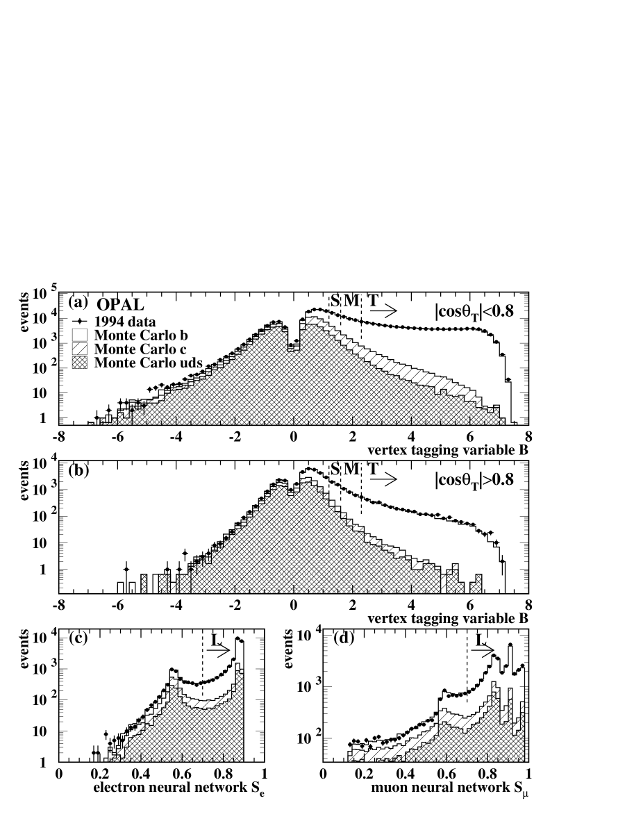
Figure 1: Distributions of (a–b) the vertex tagging variable $B$ in different regions of $|\mbox{$\cos\theta_{T}$}|$; (c) the electron tag neural network $S_{e}$; (d) the muon tag neural network $S_{\mu}$ for the 1994 data (points) and Monte Carlo simulation (histogram). The contributions from hemispheres containing light (uds), c and b quarks are indicated, and the cuts defining the hemisphere T, M, S and L tags are shown by the dashed lines. Distributions for the other years are similar.

Electrons and muons with momentum $p>2$ GeV and transverse momentum $p_{t}>1\,$GeV were also used to tag $\rm b\overline{b}$ events. Electrons were identified in the polar angle region $|\cos\theta|<0.96$ using the neural network algorithm described in [5]. The identification relies on ionisation energy loss (${\rm d}E/{\rm d}x$) measured in the tracking chamber, together with spatial and energy-momentum ($E/p$) matching between tracking and calorimetry. Photon conversions were rejected using another neural network algorithm [5]. Muons were identified in the same polar angle region by requiring a spatial match between a track reconstructed in the tracking detectors and a track segment reconstructed in the external muon chambers, as in [17].

The tagged lepton hemispheres were further enhanced in semileptonic b decays by using information from the lepton $p$ and $p_{t}$ and its degree of isolation from the rest of the jet in a neural network algorithm [18]. The distribution of the neural network output variable $S_{\ell}$ ($\ell=\rm e,\mu$) for identified electrons and muons is shown in Figure 1(c) and (d). Hemispheres were defined to be tagged with the lepton tag L if any lepton in the hemisphere had an output $S_{\ell}>0.7$, corresponding to a b-tagging efficiency of 8 % and a non-$\rm b\overline{b}$ impurity of 20 %. If a vertex T, M or S tag was also present in the hemisphere, it was ignored and the hemisphere considered only as an L tag.

Events containing at least one hemisphere with a T, M, S or L b-tag were considered selected and used for the asymmetry analysis. Each combination of tags in the two hemispheres (T-nothing, L-nothing, T-T, T-S etc.) defined a separate tagging class, making a total of 14 tagging classes. In the data, 520133 b-tagged events were selected in one of the 14 classes, with a $\rm b\overline{b}$ event tagging efficiency of about 54 %. The most important tagging classes are those with a T, L, S or M tag opposite an untagged hemisphere, which comprise 33 %, 22 %, 14 % and 13 % of the tagged data sample.

5 Tagging the b production flavour

The production flavour (b or $\rm\overline{b}$) of the b quark was determined independently in the two hemispheres of each selected event, irrespective of which hemispheres were tagged by the T, M, S or L b-tags described above. Up to four pieces of information were used per hemisphere: the momentum-weighted average track charge with two different weighting factors (evaluated for the highest energy jet in each hemisphere), the charge of a secondary vertex reconstructed in the hemisphere, and the charge of any kaon in the hemisphere, identified using ${\rm d}E/{\rm d}x$ information. The jet charges can be calculated for every hemisphere, whilst the vertex and kaon charges are only available for a subset of hemispheres. The available information was combined using a neural network algorithm to produce a single production flavour tag variable $Q$ for each hemisphere. Note that although semileptonic b decays were used to tag $\rm b\overline{b}$ events, the charge of the lepton in L-tagged hemispheres was not used in the production flavour tag $Q$, in order to reduce the correlation with the b quark asymmetry analysis based on leptons [2].

The jet charge ${Q^{\kappa}_{\rm jet}}$ was calculated for the highest energy jet in each hemisphere as:

$$\mbox{${Q^{\kappa}_{\rm jet}}$}=\frac{\sum_{i}(p^{l}_{i})^{\kappa}q_{i}}{\sum_{i}(p^{l}_{i})^{\kappa}}\,,$$

where $p^{l}_{i}$ is the longitudinal momentum component with respect to the jet axis and $q_{i}$ the charge ($\pm 1$) of track $i$, and the sum was taken over all tracks in the jet [19]. Two jet charges ${Q^{\kappa=0.5}_{\rm jet}}$ and ${Q^{\kappa=1.0}_{\rm jet}}$ were calculated for each jet, with the exponent $\kappa$ set to 0.5 and 1.0. The value $\kappa=0.5$ optimises the separation between hemispheres containing b and $\rm\overline{b}$ quarks for a single jet charge [6], and including the second jet charge with $\kappa=1.0$ provides a small amount of additional separation power, although the two jet charges are strongly correlated.

For hemispheres containing a reconstructed secondary vertex, the charge of this vertex $Q_{\rm vtx}$ was calculated as:

$$\mbox{$Q_{\rm vtx}$}=\sum_{i}w_{i}q_{i}\,,$$

and the uncertainty $\sigma_{Q_{\rm vtx}}$ as:

$$\mbox{$\sigma_{Q_{\rm vtx}}$}=\sum_{i}w_{i}(1-w_{i})q_{i}\,,$$

where $w_{i}$ is the weight for track $i$ to have come from the secondary, rather than the primary, vertex [20], and the sum was again taken over all tracks in the jet. The weights $w_{i}$ were obtained from a neural network algorithm using as input the track momentum, transverse momentum with respect to the jet axis, and impact parameters with respect to the reconstructed primary and secondary vertices, as in [6]. A well-reconstructed (small $\sigma_{Q_{\rm vtx}}$) vertex charge close to $+1$ ($-1$) indicates a $\rm B^{+}$ ($\rm B^{-}$) hadron, tagging the hemisphere as containing a $\rm\overline{b}$(b) quark, whilst a vertex charge close to zero indicates a neutral b hadron, (e.g. $\rm B^{0}$ or $\rm\bar{B}^{0}$), giving no information on the b quark production flavour. A vertex charge with large $\sigma_{Q_{\rm vtx}}$ cannot distinguish between charged and neutral b hadrons, and also provides no information on the b quark production flavour.

Charged kaons produced from the b hadron decay can also be used to tag the b production flavour, via the underlying quark decay cascade $\rm b\rightarrow c\rightarrow s$. Candidate kaon tracks were selected in the highest energy jet in each hemisphere by using ${\rm d}E/{\rm d}x$ information, requiring the track to have a probability to be consistent with a kaon of at least 5 %, and rejecting any tracks with a probability to be consistent with a pion exceeding 1 %. If more than one track in the jet was selected, the one with the highest weight $w_{i}$ to come from the secondary vertex was retained. If no secondary vertex was reconstructed in the jet, the weights were calculated using only the track momentum, transverse momentum and impact parameters with respect to the primary vertex.

The hemispheres were then categorised into one of four classes, as follows: (1) neither vertex nor kaon charge, (2) vertex charge only, (3) kaon charge only (4) both vertex and kaon charges. The available tagging variables were combined using a neural network with up to five inputs: the two jet charges ${Q^{\kappa=0.5}_{\rm jet}}$ and ${Q^{\kappa=1.0}_{\rm jet}}$, the vertex charge $Q_{\rm vtx}$ and error $\sigma_{Q_{\rm vtx}}$  and the weight $w_{i}$ of the kaon track, signed by its charge. Separate neural networks were trained for each of the four classes. The continuous tagging variable $Q$ is derived from the output $x$ of the neural network, and is defined such that

$$Q=\frac{N_{\rm\bar{b}}(x)-N_{\rm b}(x)}{N_{\rm\bar{b}}(x)+N_{\rm b}(x)}\,,$$

where $N_{\rm b}(x)$ and $N_{\rm\bar{b}}(x)$ are the number densities of Monte Carlo b and $\rm\overline{b}$ hemispheres with a particular value of $x$. Hemispheres with $Q=+1$ ($-1$) are tagged with complete confidence as being produced from $\rm\overline{b}$(b) quarks, and hemispheres with $Q=0$ are equally likely to be from either. The modulus $|Q|$ satisfies $|Q|=1-2\xi$ where $\xi$ is the ‘mis-tag’ probability, i.e. the probability to tag the production flavour incorrectly. The effects of $\rm B^{0}$ and $\rm B_{s}$ mixing contribute to the mis-tag probability, since the decay flavour of a mixed b hadron is opposite to its production flavour. A similar tagging procedure was used in [7, 8], though with leptons rather than charged kaons included in the tagging information.

The jet and vertex charge distributions are not charge symmetric, since detector effects cause differences in the rate and reconstruction of positive and negative tracks. These effects are caused by hadronic interactions in the detector material and the Lorentz angle in the tracking chambers [21]. They were removed by subtracting the mean value of each charge variable from the measured value before the calculation of $Q$. A final offset was then subtracted from $Q$ as part of the asymmetry fit procedure.

The distributions of $Q$ in the four tagging classes are shown for all selected events in the 1994 data and Monte Carlo simulation in Figure 2. Some discrepancies are visible, particularly in class 1. These are not important since the tagging power of $Q$ is measured directly from the data for $\rm b\overline{b}$ events, and the corresponding effect on charm and light quark events is covered by the physics simulation systematic uncertainties. The four classes comprise about 25 %, 36 %, 15 % and 24 % of the data sample, and have effective mistag fractions of 33.1 %, 31.2 %, 32.5 % and 29.1 %.

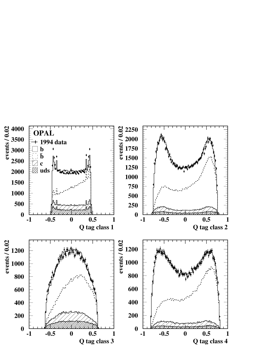
Figure 2: Distributions of the production flavour tag $Q$ in the four tagging classes for 1994 data (points) and Monte Carlo simulation (histogram). The contributions from hemispheres containing b and $\rm\overline{b}$ quarks are shown, together with the charm and light quark (uds) background. Distributions for the other years are similar.

6 Fit and Results

The procedure which is used to derive the forward-backward asymmetry $A^{\rm b}_{\rm FB}$ follows closely that in [3], the main difference being the definition of the production flavour tag $Q$. In [3], $Q$ was defined to be a jet charge with $\kappa=0.5$ and the vertex charge information was used in a separate fit. In this analysis, $Q$ is defined to be the output of the artificial neural network tag described in the preceding section, which incorporates all information from the jet, vertex and kaon charges.

In the case of a data sample consisting of only $\rm b\overline{b}$ events without contamination from lighter quarks, and neglecting acceptance effects, it can be shown that

$$\langle Q_{\rm F}-Q_{\rm B}\rangle=\mbox{$A^{\rm b}_{\rm FB}$}\cdot\delta_{\rm b}\,,$$

where $Q_{\rm F}$ and $Q_{\rm B}$ are the production flavour tags in the forward and backward hemispheres as measured in the data, and $\langle Q_{\rm F}-Q_{\rm B}\rangle$ is the mean difference of the production flavour tag values in the two hemispheres. The variable $\delta_{\rm b}$ is equal to $\langle Q_{-}-Q_{+}\rangle$, where $Q_{-}$ ($Q_{+}$) is the charge in the hemisphere containing the negatively (positively) charged primary b ($\rm\overline{b}$) quark. It measures the mean charge separation between negatively and positively charged hemispheres and is sensitive to the tagging power of $Q$ [22].

In the presence of charm and light quark backgrounds in the data sample, and in case of tagging efficiencies varying as a function of $|\cos\theta_{T}|$, the above equation must be modified:

$$\langle Q_{\rm F}-Q_{\rm B}\rangle=\sum_{{\rm flavours}\ f}s_{f}P_{f}C_{f}\delta_{f}\mbox{$A^{f}_{\rm FB}$}.$$ (1)

In this equation, $s_{f}$ is $+1$ for down-like and $-1$ for up-like quarks, $P_{f}$ is the fraction of events of flavour $f$ in the data sample, derived mainly from the data as described below, and $\delta_{f}$ is the charge separation for flavour $f$ which is determined directly from the data for $\rm b\overline{b}$ events and from Monte Carlo simulation for the other quark flavours. The factors $C_{f}$, which are taken from Monte Carlo simulation, account for variations of the asymmetry and the tagging efficiency with $\cos\theta_{T}$ and are given by

$$C_{f}=\frac{8}{3}\frac{\int\overline{\eta}_{f}(y)y\,{\rm d}y}{\int\overline{\eta}_{f}(y)(1+y^{2})\,{\rm d}y}=\frac{8}{3}\frac{\sum_{\rm events}y}{\sum_{\rm events}(1+y^{2})}\,,$$ (2)

with $y=|\cos\theta_{T}|$; $\overline{\eta}_{f}$ is the efficiency to tag an event of flavour $f$ in a given small interval of $y$. The sums run over all tagged Monte Carlo events of flavour $f$.

In the absence of correlations between the charges $Q$ measured in both hemispheres (except for primary quark charges), and if there are no charge biases, i.e. if the mean hemisphere charge of all hemispheres is zero, the mean charge separation $\delta$ can be derived directly from the data according to

$$\frac{\delta^{2}}{4}=-\langle Q_{\rm F}\cdot Q_{\rm B}\rangle.$$ (3)

In the presence of charge biases (due to detector effects as discussed in Section 5) and correlations between the hemispheres, equation (3) must be modified and becomes [22]

$$\frac{\delta^{2}}{4}=\frac{-\langle Q_{\rm F}\cdot Q_{\rm B}\rangle+\rho\cdot\sigma^{2}+\mu^{2}}{1+\rho}\,,$$

where $\mu$ and $\sigma^{2}$ are the mean and variance of the hemisphere charge for all hemispheres measured from data. The variable $\rho$ is the correlation between $Q_{-}$ and $Q_{+}$, evaluated in Monte Carlo $\rm b\overline{b}$ events and given by

$$\rho=\frac{\langle Q_{+}\cdot Q_{-}\rangle-\langle Q_{+}\rangle\cdot\langle Q_{-}\rangle}{\sigma_{Q_{+}}\sigma_{Q_{-}}}\,,$$ (4)

where $\sigma^{2}_{Q_{+}}$ and $\sigma^{2}_{Q_{-}}$ are the variances of the distributions of $Q_{+}$ and $Q_{-}$. In the presence of charm and light flavour background, the measured charge separation $\delta$ receives contributions from all flavours according to their fraction of the data sample:

$$\delta=\sum_{{\rm flavours}\ f}P_{f}\delta_{f}\,.$$ (5)

The values of $\delta_{f}$ for charm and light quarks can be derived from Monte Carlo simulation according to

$$\delta_{f}=s_{f}\cdot\langle Q_{-}-Q_{+}\rangle_{f}$$

where $\langle Q_{-}-Q_{+}\rangle_{f}$ is determined in events of flavour $f$. This allows $\delta_{\rm b}$ to be determined from equation (5) once the flavour fractions $P_{f}$ are known, and then allows the b quark asymmetry $A^{\rm b}_{\rm FB}$ to be derived by solving equation (1), using assumed values for the charm and light quark asymmetries.

These asymmetries, together with fractions $R_{f}$ of hadronic $\rm Z^{0}$ decays to each quark flavour, were set to the Standard Model expectations as calculated by ZFITTER 6.36 [23], and are given in Table 1. Since part of the data sample was taken at centre-of-mass energies above and below the $\rm Z^{0}$ peak, the values of $\langle Q_{\rm F}-Q_{\rm B}\rangle$ were calculated separately for three energy bins, allowing the corresponding values of $A^{\rm b}_{\rm FB}$ to be determined. The energy bin limits and mean centre-of-mass energy in each bin are also given in Table 1. All data were used for the calculation of $\delta_{\rm b}$ since it does not vary significantly with centre-of-mass energy.

Flavour	$R_{f}$	$A^{f}_{\rm FB}$ $(\langle\sqrt{s}\rangle=$89.50 GeV)	$A^{f}_{\rm FB}$ $(\langle\sqrt{s}\rangle=$91.26 GeV)	$A^{f}_{\rm FB}$ $(\langle\sqrt{s}\rangle=$92.91 GeV)
		(88.40–90.40 GeV)	(91.05–91.50 GeV)	(91.70–94.00 GeV)
$\rm b\overline{b}$	0.2155	–	–	–
$\rm c\overline{c}$	0.1726	$-0.0309$	0.0633	0.1211
$\rm s\overline{s}$	0.2196	0.0595	0.0964	0.1189
$\rm u\overline{u}$	0.1728	$-0.0308$	0.0632	0.1207
$\rm d\overline{d}$	0.2196	0.0595	0.0964	0.1189

Table 1: Values for $R_{f}$ for bottom, charm and light quarks and forward-backward asymmetries for charm and light quarks as calculated from ZFITTER [23] for the three different energy bins. For each energy bin, the mean energy and the bin limits are also given.

The above procedure was applied separately to each of the 14 tag classes and in five bins of $|\mbox{$\cos\theta_{T}$}|$ with bin edges at $|\mbox{$\cos\theta_{T}$}|=0$, 0.2, 0.4, 0.6, 0.8 and 0.95. The flavour fractions $P_{f}$ were determined simultaneously for all 14 tag classes in each $|\mbox{$\cos\theta_{T}$}|$ bin using the measured tagging rates for each class. Within the tagging class $kl$, where $k$,$l$={T, M, S, L or nothing }, i.e. tagged in one hemisphere by b-tag $k$ and in the other hemisphere by b-tag $l$, the fraction of events $P^{kl}_{f}$ of flavour $f$={b,c,uds} is given by

$$P^{kl}_{f}=\frac{R_{f}D^{kl}_{f}\epsilon^{k}_{f}\epsilon^{l}_{f}}{\sum_{i}R_{i}D^{kl}_{i}\epsilon^{k}_{i}\epsilon^{l}_{i}}\,,$$ (6)

where the sum in the denominator runs over b, c and light quark (uds) flavours, $\epsilon_{f}^{k}$ is the hemisphere tagging efficiency of tag $k$ for flavour $f$, and the correlation $D_{f}^{kl}$ is defined by $D^{kl}_{f}=\epsilon^{kl}_{f}/(\epsilon^{k}_{f}\epsilon^{l}_{f})$, where $\epsilon^{kl}_{f}$ is the efficiency for an event of flavour $f$ to be tagged by tag $k$ in one hemisphere and tag $l$ in the other hemisphere. Deviations of $D^{kl}_{f}$ from unity account for the fact that the tagging in the two hemispheres is not completely independent. For light quark events, these correlations have negligible effect and are set to one. The fraction of hemispheres $f_{s}^{i}$ in the $|\mbox{$\cos\theta_{T}$}|$ bin that are tagged by b-tag $i$, and the fraction of events $f_{d}^{kl}$ tagged by b-tag $k$ in one hemisphere and b-tag $l$ in the other hemisphere are then given by

$$f_{s}^{i} = \epsilon_{\rm b}^{i}\mbox{$R_{\rm b}$}+\epsilon_{\rm c}^{i}\mbox{$R_{\rm c}$}+\epsilon_{\rm uds}^{i}(1-\mbox{$R_{\rm b}$}-\mbox{$R_{\rm c}$})\,,$$

$$f_{d}^{kl} = \epsilon_{\rm b}^{k}\epsilon_{\rm b}^{l}D_{\rm b}^{kl}\mbox{$R_{\rm b}$}+\epsilon_{\rm c}^{k}\epsilon_{\rm c}^{l}D_{\rm c}^{kl}\mbox{$R_{\rm c}$}+\epsilon_{\rm uds}^{k}\epsilon_{\rm uds}^{l}(1-\mbox{$R_{\rm b}$}-\mbox{$R_{\rm c}$})\ .$$

This system of equations was solved using a maximum likelihood fit. The uds tagging efficiencies and all correlation terms were fixed to values determined from Monte Carlo simulation, and the b- and c-tagging efficiencies of the T, M, S and L tags were allowed to vary in order to minimise the difference between the observed and predicted tag fractions. Then the flavour fractions $P_{f}^{kl}$ for each tagging class were calculated from equation (6), defining the untagged efficiencies for each flavour as $\epsilon^{\rm nothing}_{f}=1-\epsilon^{\rm T}_{f}-\epsilon^{\rm M}_{f}-\epsilon^{\rm S}_{f}-\epsilon^{\rm L}_{f}$. The values for $R_{\rm b}$ and $R_{\rm c}$ were computed using ZFITTER (see Table 1).

The asymmetry fit procedure was applied separately to the events collected in each of the five $|\mbox{$\cos\theta_{T}$}|$ bins and 14 tag classes, resulting in 70 different values for $A^{\rm b}_{\rm FB}$ for each energy bin and data taking period (1991–2, 1993, 1994, 1995 and 1996–2000). All the $A^{\rm b}_{\rm FB}$ measurements for each energy point were then combined, weighted according to their statistical errors. The mean charge flow $\langle Q_{\rm F}-Q_{\rm B}\rangle$ as a function of $|\mbox{$\cos\theta_{T}$}|$ is shown for $\rm Z^{0}$ peak events with either hemisphere tagged by a L, S, M or T tag in Figure 3(a–d), and for all tagged events at the off-peak energy points in Figure 3(e) and (f). The expected distribution from the result of the asymmetry fit is also shown in each case.

Figure 3: The mean charge flow as a function of $|\mbox{$\cos\theta_{T}$}|$ in the entire dataset (points with error bars showing the statistical errors), together with the prediction from the asymmetry fit (histogram). Figures (a–d) show the distributions for $\rm Z^{0}$ peak events tagged in either hemisphere with an L, S, M or T tag, whilst (e) and (f) show all tagged events at the two off-peak energy points.

These fitted asymmetry values do not correspond directly to the b quark forward-backward asymmetry because of the effects of gluon radiation from the primary quark pair and the approximation of the original quark direction by the experimentally measured thrust axis [24]. The effects of gluon radiation have been calculated to second order in $\alpha_{s}$, using the parton level thrust axis to define the asymmetry [25]. The correction needed to go from the parton level to the hadron level thrust axis (calculated using all final state particles without detector effects) has been determined using Monte Carlo hadronisation models [24]. However, these corrections cannot be applied directly to this analysis, since the determination of the production flavour tagging power directly from the data already accounts for most of the effects of gluon radiation. Therefore, a large sample of Monte Carlo simulated events was used to determine the correction to the measured asymmetries directly, by comparing the asymmetry fit results on this sample with the true primary b quark asymmetry. This correction factor was rescaled so as to take the quark to hadron level correction from the theoretical calculation discussed above, since the calculation is expected to be more accurate than the Monte Carlo simulation for this part of the overall correction. Combining all effects, the measured asymmetries were scaled by $0.9923\pm 0.0063\pm 0.0038$ to determine the quark level asymmetries, where the first error is due to theoretical uncertainties in the quark to hadron level calculation [24, 26] and the second to Monte Carlo statistics.

The measured asymmetry values, after correcting to the quark level, are:

$A^{\rm b}_{\rm FB}$	=	$0.0582\pm 0.0153$	at  $\sqrt{s}=89.50$ GeV
$A^{\rm b}_{\rm FB}$	=	$0.0977\pm 0.0036$	at  $\sqrt{s}=91.26$ GeV
$A^{\rm b}_{\rm FB}$	=	$0.1221\pm 0.0123$	at  $\sqrt{s}=92.91$ GeV

where the errors are statistical only.

7 Systematic errors

Systematic errors on $A^{\rm b}_{\rm FB}$ arise from uncertainties in the input quantities which are taken from Monte Carlo, namely the b-tagging correlations $D_{\rm b}$, the production flavour tag correlations $\rho_{\rm b}$, the charge separations $\delta_{f}$ for charm and light quark events, the light quark tagging efficiencies $\epsilon_{\rm uds}$ and the efficiency correction factors $C_{f}$. Additional uncertainties result from material asymmetries in the detector and the calculation of the QCD corrections to the raw measured asymmetries. The systematic errors are summarised in Table 2 and discussed in more detail below.

Uncertainty	$\langle\sqrt{s}\rangle=$ 89.50 GeV	$\langle\sqrt{s}\rangle=$ 91.26 GeV	$\langle\sqrt{s}\rangle=$ 92.91 GeV
b fragmentation	0.00021	0.00033	0.00053
$\rm B_{s}$ rate	0.00006	0.00005	0.00007
b baryon rate	0.00002	0.00003	0.00006
b lifetimes	0.00001	0.00001	0.00001
b charged multiplicity	0.00002	0.00001	0.00003
$D_{\rm b}$ kinematics	0.00004	0.00019	0.00029
$D_{\rm b}$ geom-kin independence	0.00009	0.00072	0.00122
$\rho_{\rm b}$ flavour tag correlation	0.00065	0.00089	0.00118
Total b physics	0.00069	0.00121	0.00180
c fragmentation	0.00008	0.00016	0.00025
$\rm D^{+}$ production fraction	0.00005	0.00014	0.00022
$\rm D_{s}$ production fraction	0.00006	0.00016	0.00024
$\Lambda_{\rm c}$ production fraction	0.00004	0.00015	0.00023
$\rm D^{*}$, $\rm D^{**}$ fractions	0.00008	0.00006	0.00013
c lifetimes	0.00001	0.00001	0.00002
c charged multiplicities	0.00003	0.00014	0.00025
$\rm D\rightarrow K^{0},\Lambda$ multiplicities	0.00004	0.00024	0.00042
c neutral multiplicities	0.00005	0.00032	0.00054
$\rm D\rightarrow K^{+}$ multiplicity	0.00002	0.00013	0.00020
Total c physics	0.00017	0.00054	0.00090
Strange particle production	0.00001	0.00003	0.00004
Light quark fragmentation	0.00012	0.00012	0.00012
g$\rightarrow\rm{b\overline{b}}$ rate	0.00001	0.00007	0.00006
g$\rightarrow\rm{c\overline{c}}$ rate	0.00001	0.00008	0.00014
$r$-$\phi$ tracking resolution	0.00065	0.00068	0.00056
$r$-$z$ tracking resolution	0.00036	0.00033	0.00048
Silicon hit efficiency	0.00044	0.00047	0.00082
Silicon alignment	0.00002	0.00003	0.00009
Electron fake rate	0.00002	0.00014	0.00021
Muon fake rate	0.00004	0.00022	0.00034
Material asymmetry	0.00009	0.00009	0.00009
Total detector	0.00087	0.00093	0.00117
QCD and thrust axis correction	0.00043	0.00073	0.00091
Event selection bias	0.00002	0.00011	0.00016
LEP centre-of-mass energy	0.00008	0.00010	0.00003
Total systematic uncertainty	0.00121	0.00179	0.00252

Table 2: Summary of systematic uncertainties on the measured values of $A^{\rm b}_{\rm FB}$ for the three different energy bins.

7.1 Hemisphere correlations

The following uncertainties in the simulation of b hadron production and decay affect the estimates of both the b-tag correlations $D_{\rm b}$ and the production flavour tag correlations $\rho_{\rm b}$. They were estimated by reweighting the Monte Carlo sample used to derive the correlations and repeating the asymmetry fit using the modified parameters.

b quark fragmentation:

The Monte Carlo was reweighted so as to vary the average scaled energy $\langle{x_{E}}\rangle$ of weakly decaying b hadrons in the range $\mbox{$\langle{x_{E}}\rangle$}=0.702\pm 0.008$, as determined by the LEP electroweak working group [26]. The fragmentation functions of Peterson et al., Collins and Spiller, Kartvelishvili et al. and the Lund group [15, 27] were each used as models to determine the event weights, and the largest observed variations in $A^{\rm b}_{\rm FB}$ were assigned as the systematic errors.

b hadron production fractions:

The fractions of b quarks hadronising to form $\rm B_{s}$ mesons and $\rm\Lambda_{b}$ baryons were varied in the ranges $f(\rm b\rightarrow\mbox{$\rm B_{s}$})=(10.7\pm 1.4)$ % and $f(\rm b\rightarrow\mbox{$\rm\Lambda_{b}$})=(11.6\pm 2.0)$ % [28].

b lifetimes:

The lifetimes of b mesons were varied by $\pm 0.02$ ps and b baryons by $\pm 0.05$ ps, based on the uncertainties on the measured values [28].

b decay charged multiplicity:

The average charged decay multiplicity of b hadrons was varied by $\pm 0.062$, reflecting the accuracy of the measurements by LEP experiments [26].

Hemisphere b-tagging correlations $D_{\rm b}$ were extensively studied for the measurement of $R_{\rm b}$ [5] and found to result from two main sources: (i) kinematical correlations between the momenta of the two b quarks in a $\rm b\overline{b}$ event (due to hard gluon radiation and soft particles produced in the hadronisation of the two b quarks); and (ii) geometrical correlations caused by the strong dependence of the b-tagging efficiency on $|\mbox{$\cos\theta_{T}$}|$. Kinematical correlations were found to be small, and modelled in the Monte Carlo to a precision of $\Delta\mbox{$D_{\rm b}$}=0.0022$ [5]. The systematic error for the $A^{\rm b}_{\rm FB}$ analysis was assessed by simultaneously changing the b-tag correlations $D_{\rm b}$ for all 70 analysis bins by $\pm 0.0022$ and repeating the asymmetry fit.

The geometrical correlation contributions to $D_{\rm b}$ were measured directly from the data in each of the 70 analysis bins, using the rate of tagged events as a function of the polar and azimuthal angles of the thrust axis, as described in [5]. At high $|\mbox{$\cos\theta_{T}$}|$, the geometrical correlations are large, rising to around $\mbox{$D_{\rm b}$}-1=+0.5$ for the T-T double-tagged events at $|\mbox{$\cos\theta_{T}$}|>0.9$. Here, the assumption of independent geometrical and kinematic correlations breaks down, and their sum overestimates the overall correlation determined directly from the Monte Carlo single and double tag efficiencies. To account for possible Monte Carlo mis-modelling of this effect, the full difference between the correlation component sum and the overall correlation was taken as an additional systematic error on $D_{\rm b}$, for all analysis bins where this difference was statistically significant. To assess the corresponding systematic error on $A^{\rm b}_{\rm FB}$, the asymmetry fit was repeated with the $D_{\rm b}$ correlations for all such bins shifted simultaneously.

The largest single contribution to the overall systematic uncertainty arises from the correlation $\rho_{\rm b}$ between the production flavour tag determinations in the hemispheres of the primary b and $\rm\overline{b}$ quarks, $Q_{-}$ and $Q_{+}$ (see equation (4)). The values of $\rho_{\rm b}$ are typically between zero and $-10$ %, depending on tagging class and $|\mbox{$\cos\theta_{T}$}|$. The origin of the correlation is primarily events with significant gluon radiation, which reduces the momenta of both b hadrons, and may also lead to a third jet shared between the two hemispheres. Both of these effects reduce the average tagging power in both hemispheres of the event, leading to a tagging correlation. This can be seen in Figure 4(a), which shows the overall correlation $\rho_{\rm b}$ averaged over all 70 tagging bins as a function of thrust. The correlation is stronger in events with low thrust values, corresponding to significant gluon radiation and a three-jet topology.

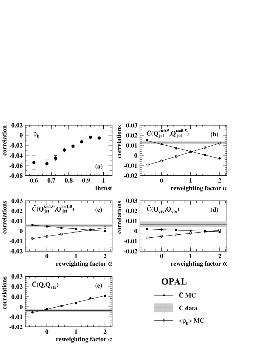
Figure 4: Studies of the production flavour tag hemisphere correlations $\rho_{\rm b}$ (see text): (a) Average value of $\rho_{\rm b}$ as a function of thrust; (b–d) correlation test variables $\tilde{C}$ for ${Q^{\kappa=0.5}_{\rm jet}}$, ${Q^{\kappa=1.0}_{\rm jet}}$ and $Q_{\rm vtx}$ in data (with shaded error band) and Monte Carlo (as a function of correlation reweighting factor $\alpha$), together with corresponding values of $\rho_{\rm b}$; (e) correlation between $Q_{\rm vtx}$ and production flavour tag $Q$ in data and Monte Carlo (as a function of correlation reweighting factor $\alpha$). The lines through the points in Figures (b–e) show the result of linear fits used to parameterise the dependence of the correlations on $\alpha$.

In order to check the modelling of the correlation $\rho_{\rm b}$ in the Monte Carlo simulation, the variables that contribute to the correlation were determined, and studied using a reweighting procedure. For a variable $X$ possibly contributing to $\rho_{\rm b}$, the correlation

$$C_{X}=\frac{\langle X_{+}\cdot X_{-}\rangle-\langle X_{+}\rangle\cdot\langle X_{-}\rangle}{\sigma_{X_{+}}\sigma_{X_{-}}}$$

was determined in Monte Carlo events, where $X_{+}$ and $X_{-}$ are the values of the variable in the hemispheres of the primary $\rm\overline{b}$ and b quarks. Event weights were then determined in small bins of $X_{+}$ and $X_{-}$ such that the correlation between $X_{+}$ and $X_{-}$ could be removed, and the effect on the overall correlation $\rho_{\rm b}$ was studied. Using this procedure, the two jet charges ${Q^{\kappa=0.5}_{\rm jet}}$ and ${Q^{\kappa=1.0}_{\rm jet}}$ and the vertex charge $Q_{\rm vtx}$ were identified to be the relevant variables contributing to the non-zero value of $\rho_{\rm b}$.

Since the determination of $C_{X}$ is possible only in Monte Carlo events, where the hemisphere of the original b quark is known, an additional set of correlations were defined according to

$$\tilde{C}_{X}=\frac{\langle|X_{F}|\cdot|X_{B}|\rangle-\langle|X_{F}|\rangle\cdot\langle|X_{B}|\rangle}{\sigma_{X_{F}}\sigma_{X_{B}}}\,,$$

where $X_{F}$ and $X_{B}$ are the values of the variable $X$ in the forward and backward hemispheres. These $\tilde{C}_{X}$ are sensitive to the correlation $C_{X}$ and can also be measured in data, to check the Monte Carlo modelling of the hemisphere correlation of the variable $X$. This was done by applying scale factors $\alpha$ to the weights used to remove the correlation, and calculating $\tilde{C}_{X}$ in Monte Carlo events as a function of $\alpha$. The values of $\tilde{C}_{X}$ were then compared to $\tilde{C}_{X}$ measured in data to determine the range of $\alpha$ allowed by the data. This procedure is illustrated in Figure 4(b–d), which show for the three variables of interest the data value of $\tilde{C}_{X}$ together with the Monte Carlo values of $\tilde{C}_{X}$ and the overall correlation $\rho_{\rm b}$ as a function of the scale factor $\alpha$.

For the two jet charges ${Q^{\kappa=0.5}_{\rm jet}}$ and ${Q^{\kappa=1.0}_{\rm jet}}$, the agreement between data and unweighted Monte Carlo is good, and the correlations $\tilde{C}_{X}$ are sensitive measurements of the corresponding contributions to $\rho_{\rm b}$. The systematic error on $A^{\rm b}_{\rm FB}$ was calculated by varying the amount of reweighting in the range allowed by the data, recalculating the values of $\rho_{\rm b}$ for all 70 analysis bins and refitting the asymmetries. This procedure results in systematic uncertainties of 0.00048 and 0.00070 on $A^{\rm b}_{\rm FB}$ in the $\rm Z^{0}$ peak energy bin for the jet charges ${Q^{\kappa=0.5}_{\rm jet}}$ and ${Q^{\kappa=1.0}_{\rm jet}}$ respectively. For the vertex charge $Q_{\rm vtx}$, Figure 4(d) shows that data and Monte Carlo are consistent (within two standard deviations), but that the size of the statistical error is too large and the effect on $\rho_{\rm b}$ too weak to draw precise conclusions about the Monte Carlo modelling of the $Q_{\rm vtx}$ correlation. Figure 4(e) shows a more sensitive variable, the correlation $\tilde{C}$ of the vertex charge in one hemisphere and the production flavour tag in the other hemisphere, where again good agreement between data and Monte Carlo is seen, giving confidence in the Monte Carlo description of the vertex charge correlations. However, since this test is more indirect and cannot be directly applied to the vertex charge reweighting, the systematic error on $A^{\rm b}_{\rm FB}$ is assessed by reweighting based directly on the vertex charges in the two hemispheres, so as to increase or decrease the correlation $\tilde{C}_{Q_{\rm vtx}}$ by 50 %. This gives an additional systematic error on $A^{\rm b}_{\rm FB}$ of 0.00026. Adding the contributions of the three variables in quadrature gives a total error due to the modelling of the $\rho_{\rm b}$ hemisphere correlations of 0.00089.

7.2 Detector Simulation

Both the tagging correlations $D_{\rm b}$ and $\rho_{\rm b}$, and the other input parameters $\delta$, $\epsilon_{\rm uds}$ and $C_{f}$ are sensitive to details of the detector simulation, in particular the tracking and lepton identification performance.

Tracking resolution:

The error due to uncertainties in the tracking resolution was assessed by applying a global 10 % degradation to the resolution of all tracks, independently in the $r$-$\phi$ and $r$-$z$ planes, as in [5]. This degradation accounts for the discrepancies between data and Monte Carlo backward tagging rates seen in Figure 1(a) and (b). The resolution is also sensitive to the efficiency for associating silicon hits to tracks, which was varied by $\pm 1$ % in the $r$-$\phi$ and $\pm 2$ % in the $r$-$z$ planes to cover residual discrepancies between data and Monte Carlo hit association rates.

Silicon alignment:

The b-tagging performance is sensitive to knowledge of the radial positions of the silicon microvertex detector wafers, which are known to a precision of $\pm 20\,\mu$m from studies of cosmic ray events [5]. The corresponding uncertainty is assessed by displacing one or both barrels radially by $20\,\mu$m in the simulation.

Lepton identification:

The light quark tagging efficiencies $\epsilon_{\rm uds}$ for the L tag are sensitive to the number of charged hadrons mis-identified as electrons and muons, which is modelled in the Monte Carlo to precisions of $\pm 21\,$% for fake electrons and $\pm 9$ % for fake muons [5]. The analysis is not sensitive to the Monte Carlo description of the efficiencies for identifying real leptons, since these occur primarily in $\rm b\overline{b}$ and $\rm c\overline{c}$ events, whose tagging efficiencies are measured directly from the data.

7.3 Charm and light quark physics

The following uncertainties in the simulation of charm physics affect the asymmetry analysis through the input values of $\delta_{c}$, the charge separations in $\rm c\overline{c}$ events. The effect of corresponding uncertainties on the charm hemisphere b-tagging and production flavour tagging correlations is negligible.

Charm fragmentation:

The Monte Carlo was reweighted so as to vary the mean scaled energy $\langle{x_{E}}\rangle$ of charm hadrons in $\rm c\overline{c}$ events in the range $\mbox{$\langle{x_{E}}\rangle$}=0.484\pm 0.008$ [26], using the same four fragmentation functions as for $\rm b\overline{b}$ events.

Charm hadron production fractions:

The production fractions of the weakly decaying charm hadrons were varied according to the measurements performed at LEP [29], as averaged by the LEP electroweak working group [26]. The contribution from $\Lambda^{+}_{\rm c}$ was scaled by $1.15\pm 0.05$ to account for other weakly decaying charm baryons. The dependence on the production rates of excited charm states was determined by varying the fractions of charm quarks hadronising to produce $\rm D^{*+}$, $\rm D^{*0}$ and $\rm D_{s}^{*}$ in the ranges $0.239\pm 0.007$ [30], $0.218\pm 0.071$ [31] and $0.13\pm 0.13$ [31] whilst keeping the production fractions of weakly decaying charm hadrons constant. The dependence on the production of orbitally-excited charm states ($\rm D^{**}$) was found to be negligible.

Charm hadron lifetimes:

The lifetimes of the weakly decaying charm hadrons were varied separately according to the measured values [28].

Charm hadron decay multiplicities:

The average charged hadron decay multiplicities of $\rm D^{+}$, $\rm D^{0}$ and $\rm D_{s}^{+}$ mesons were varied according to the measurements of MARK III [32]. The charged decay multiplicity of charm baryons, for which no measurements are available, was varied by $\pm 0.5$. The number of $\pi^{0}$ produced in D meson decays were also varied according to the available measurements [32]. The branching ratio of charm hadrons to long-lived neutral strange particles ($\rm K^{0}$ and $\Lambda$) were varied according to the uncertainties quoted in [28]. In each case, the other branching ratios were held constant whilst the branching ratio in question was varied.

Charged kaon production in charm decays:

The tagging performance of the production flavour tag in $\rm c\overline{c}$ events is sensitive to the number of charged kaons produced in D meson decays. These were varied according to the measured values [28].

Uncertainties in the simulation of light quark events affect both the tagging efficiencies $\epsilon_{\rm uds}$ and the charge separations $\delta_{\rm u}$, $\delta_{\rm d}$ and $\delta_{\rm s}$. The inclusive production rates of $\rm K^{0}$ mesons and $\Lambda$ and other weakly decaying hyperons were varied in the Monte Carlo by $\pm 3.4$ %, $\pm 6.5$ % and $\pm 11.5$ % respectively, corresponding to the precision of the OPAL measurements [33] combined with an additional uncertainty to take into account the extrapolation of the inclusive production rates to light quark events only. Additionally, HERWIG 6.2 [34] and ARIADNE 4.08[35] were used as alternative fragmentation models for the simulation of light quark events.

The production of heavy quarks via the gluon splitting processes $\rm g\rightarrow\mbox{$\rm c\overline{c}$}$ and $\rm g\rightarrow\mbox{$\rm b\overline{b}$}$ affects the properties of both charm and light quark events. The rates were varied independently in the ranges $f(\rm g\rightarrow\mbox{$\rm c\overline{c}$})=(2.96\pm 0.38)$ % and $f(\rm g\rightarrow\mbox{$\rm b\overline{b}$})=(0.254\pm 0.051)$ % according to LEP and SLD measurements [26].

7.4 Other uncertainties

The parameters $C_{f}$ which correct for the variation of tagging efficiency with $|\mbox{$\cos\theta_{T}$}|$ within each bin are calculated separately for each flavour using Monte Carlo simulation (see equation (2)). The simulation was checked by studying the rate of tagged events as a function of $|\mbox{$\cos\theta_{T}$}|$ within each of the 70 analysis bins, and reweighting the Monte Carlo b-tagging efficiency in small bins of $|\mbox{$\cos\theta_{T}$}|$ to reproduce the data distribution. The flavour dependence of the efficiency corrections was checked by setting all charm and light quark $C_{f}$ parameters to the corresponding $C_{\rm b}$. The resulting changes in the fitted values of $A^{\rm b}_{\rm FB}$ were negligible in both cases.

As discussed in section 5, the jet and vertex charge distributions are not charge-symmetric due to detector effects. A difference in the amount of detector material in the forward and backward hemispheres could lead to different offsets in the two hemispheres and bias the measured value of $A^{\rm b}_{\rm FB}$. This material asymmetry was measured by studying the rate of identified photon conversions as a function of $\cos\theta_{T}$. For $|\mbox{$\cos\theta_{T}$}|<0.8$, the conversion asymmetry was found to be consistent with zero to a precision of $\pm 0.3$ %. For $|\mbox{$\cos\theta_{T}$}|>0.8$, the backward hemisphere was found to contain $7.2\pm 0.5$ % more material than the forward hemisphere, due to readout electronics and cabling. The systematic error on $A^{\rm b}_{\rm FB}$ was calculated by assuming that all of the jet charge offsets are due to material effects and differentially shifting them in the forward and backward hemispheres according to the measured material asymmetries as a function of $|\mbox{$\cos\theta_{T}$}|$.

The correction from the asymmetry measured using the experimental thrust axis to the primary b quark asymmetry is known to a precision of 0.74 %, including both theoretical uncertainties and Monte Carlo statistics. Note that the full size of the theoretical error is used, even though part of the gluon radiation correction is absorbed by the determination of the tagging power from the data, as discussed in Section 6.

The hadronic event selection requirements are $(0.25\pm 0.15)$ % more efficient for $\rm b\overline{b}$ events than for charm and light quark events [5], due mainly to the requirement of at least seven charged tracks. This leads to a small uncertainty on the flavour composition of the sample, and a corresponding error on $A^{\rm b}_{\rm FB}$. The LEP centre of mass energy is known to a precision of 18 MeV for the $\rm Z^{0}$ peak running in 1992, around 5 MeV for 1993–95 and 12 MeV for the $\rm Z^{0}$ calibration data taken in 1996–2000 [36]. Taking year-to-year correlations into account, and assuming the Standard Model dependence of $A^{\rm b}_{\rm FB}$ on $\sqrt{s}$, this leads to the uncertainties given in Table 2 on the asymmetries at the quoted values of $\sqrt{s}$.

The asymmetries measured in each year of the data, and in different tag classes and $|\mbox{$\cos\theta_{T}$}|$ bins are consistent. The results were found to be stable when the b-tagging cuts defining the different tag classes T, M, S and L were varied, and no additional systematic error is assigned. The fit was also tested on large samples of simulated Monte Carlo events with different true asymmetry values, and no evidence of a bias was seen. As a further cross-check, the rates of single- and double-tagged events were used to measure $R_{\rm b}$ as a function of $|\mbox{$\cos\theta_{T}$}|$ and tag type, and results consistent with the world-average value of $R_{\rm b}$ were obtained in all cases.

Derivative	$\langle\sqrt{s}\rangle=$ 89.50 GeV	$\langle\sqrt{s}\rangle=$ 91.26 GeV	$\langle\sqrt{s}\rangle=$ 92.91 GeV
d$A^{\rm b}_{\rm FB}$/d$A\rm_{FB}^{d}$	$-0.0175$	$-0.0166$	$-0.0168$
d$A^{\rm b}_{\rm FB}$/d$A\rm_{FB}^{u}$	$0.0221$	$0.0215$	$0.0222$
d$A^{\rm b}_{\rm FB}$/d$A\rm_{FB}^{s}$	$-0.0222$	$-0.0224$	$-0.0222$
d$A^{\rm b}_{\rm FB}$/d$A\rm_{FB}^{c}$	$0.0686$	$0.0695$	$0.0694$
d$A^{\rm b}_{\rm FB}$/d$R\rm_{u}$	$0.0032$	$0.0215$	$0.0331$
d$A^{\rm b}_{\rm FB}$/d$R\rm_{s}$	$0.0000$	$0.0000$	$0.0000$
d$A^{\rm b}_{\rm FB}$/d$R\rm_{c}$	$0.0030$	$0.0134$	$0.0202$
d$A^{\rm b}_{\rm FB}$/d$R\rm_{b}$	$-0.0692$	$-0.3482$	$-0.5104$

Table 3: Derivatives of $A^{\rm b}_{\rm FB}$ with respect to the assumed Standard Model parameters, for each energy bin. The value of $R_{\rm d}$ is constrained to $1-\mbox{$R_{\rm b}$}-\mbox{$R_{\rm c}$}-R_{\rm u}-R_{\rm s}$.

The fitted asymmetry values depend on the assumed values for the fraction of hadronic $\rm Z^{0}$ decays to each quark flavour, and the charm and light quark asymmetries at each energy point. The values used are given in Table 1, and the derivatives of the measured asymmetries with respect to these parameters are given in Table 3. Taking the values of $R_{\rm b}$  $R_{\rm c}$ and $A^{\rm c}_{\rm FB}$ from measurements [28] rather than ZFITTER would result in additional uncertainties on $A^{\rm b}_{\rm FB}$ at $\sqrt{s}=91.26$ GeV of 0.00026, 0.00006 and 0.00031 for $R_{\rm b}$, $R_{\rm c}$ and $A^{\rm c}_{\rm FB}$ respectively.

8 Conclusions

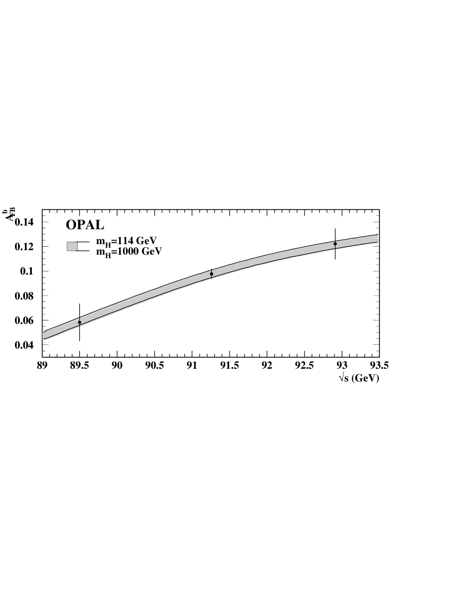
Figure 5: The measured b quark asymmetry as a function of energy (points with error bars showing both statistical and systematic errors), together with the Standard Model expectation calculated using ZFITTER [23], with the Higgs mass varied between 114 GeV and 1000 GeV.

The b quark forward-backward asymmetry has been measured using an inclusive tag at three energy points around the $\rm Z^{0}$ peak. The results, corrected to the primary quark level, are:

$A^{\rm b}_{\rm FB}$	=	$0.0582\pm 0.0153\pm 0.0012$	at  $\sqrt{s}=89.50$ GeV
$A^{\rm b}_{\rm FB}$	=	$0.0977\pm 0.0036\pm 0.0018$	at  $\sqrt{s}=91.26$ GeV
$A^{\rm b}_{\rm FB}$	=	$0.1221\pm 0.0123\pm 0.0025$	at  $\sqrt{s}=92.91$ GeV

where in each case the first error is statistical and the second systematic. The results are shown as a function of $\sqrt{s}$ in Figure 5, together with the Standard Model expectation calculated using ZFITTER [23]. Using the ZFITTER prediction for the dependence of $A^{\rm b}_{\rm FB}$ on $\sqrt{s}$, the three measurements are shifted to $m_{\rm Z}$ (91.19 GeV), averaged and corrected for initial state radiation, $\gamma$ exchange, $\gamma-\mbox{$\rm Z^{0}$}$ interference and b quark mass effects. The resulting value for the $\rm Z^{0}$ pole asymmetry $A^{\rm b,0}_{\rm FB}$ is

$$\mbox{$A^{\rm b,0}_{\rm FB}$}=0.1002\pm 0.0034\pm 0.0018$$

where again the first error is statistical and the second systematic. Within the framework of the Standard Model, this corresponds to an effective weak mixing angle for electrons of

$$\mbox{$\rm\sin^{2}\theta_{W}^{eff,e}$}=0.23205\pm 0.00068\,.$$

This result is one of the most precise measurements of the b quark forward-backward asymmetry to date. It is in agreement with, and supersedes, the previous OPAL result using jet and vertex charge [3], and is also in agreement with the OPAL measurement using leptons [2] and other measurements of $A^{\rm b}_{\rm FB}$ at LEP [4].

References

- [1] Z Physics at LEP1, volume 1, edited by G. Altarelli, CERN 89-08, 1989.
- [2] OPAL collaboration, G. Alexander et al., Z. Phys. C70 (1996) 357.
- [3] OPAL collaboration, K. Ackerstaff et al., Z. Phys. C75 (1997) 385.
-
[4]
ALEPH collaboration, A. Heister et al., Eur. Phys. J. C22 (2001) 201;
ALEPH collaboration, A. Heister et al., Eur. Phys. J. C24 (2002) 177;
DELPHI collaboration, P. Abreu et al., Z. Phys. C65 (1995) 569;
DELPHI collaboration, P. Abreu et al., Eur. Phys. J. C9 (1999) 367;
DELPHI collaboration, P. Abreu et al., Eur. Phys. J. C10 (1999) 219;
L3 collaboration, O. Adriani et al., Phys. Lett. B292 (1992) 454;
L3 collaboration, M. Acciarri et al., Phys. Lett. B448 (1999) 152. - [5] OPAL collaboration, G. Abbiendi et al., Eur. Phys. J. C8 (1999) 217.
- [6] OPAL collaboration, K. Ackerstaff et al., Eur. Phys. J. C5 (1998) 379.
- [7] OPAL collaboration, G. Abbiendi et al., Eur. Phys. J. C12 (2000) 609.
- [8] OPAL collaboration, G. Abbiendi et al., Phys. Lett. B493 (2000) 266.
-
[9]
OPAL collaboration, K. Ahmet et al., Nucl. Instrum. Methods A305 (1991) 275;
P.P. Allport et al., Nucl. Instrum. Methods A324 (1993) 34. - [10] P.P. Allport et al., Nucl. Instrum. Methods A346 (1994) 476.
- [11] S. Anderson et al., Nucl. Instrum. Methods A403 (1998) 326.
- [12] OPAL collaboration, R. Akers et al., Z. Phys. C63 (1994) 197.
- [13] T. Sjöstrand, Comp. Phys. Comm. 82 (1994) 74.
- [14] OPAL collaboration, G. Alexander et al., Z. Phys. C69 (1996) 543.
- [15] C. Peterson, D. Schlatter, I. Schmitt and P. Zerwas, Phys. Rev. D27 (1983) 105.
- [16] J. Allison et al., Nucl. Instrum. Methods A317 (1992) 47.
- [17] OPAL collaboration, P.D. Acton et al., Z. Phys. C58 (1993) 523.
- [18] OPAL collaboration, R. Akers et al., Z. Phys. C66 (1995) 555.
- [19] R.D. Field and R.P. Feynman, Nucl. Phys. B136 (1978) 1.
- [20] OPAL collaboration, R. Akers et al., Z. Phys. C66 (1995) 19.
- [21] OPAL collaboration, K. Ackerstaff et al., Z. Phys. C76 (1997) 401.
- [22] OPAL collaboration, R. Akers et al., Z. Phys. C67 (1995) 365.
-
[23]
D. Bardin et al., ZFITTER: An analytical program for fermion pair production
in annihilation, CERN-TH 6443/92, hep-ph/9412201 (1992);
D. Bardin et al., Comp. Phys. Comm. 133 (2001) 229;
The input parameters used were GeV, GeV and GeV. - [24] LEP heavy flavour working group, D. Abbaneo et al., Eur. Phys. J. C4 (1998) 185.
-
[25]
G. Altarelli and B. Lampe, Nucl. Phys. B391 (1993) 3;
V. Ravindran and W.L. van Neerven, Phys. Lett. B445 (1998) 206;
S. Catani and M.H. Seymour, JHEP 9907 (1999) 023. -
[26]
The LEP collaborations, ALEPH, DELPHI, L3 and OPAL,
Nucl. Instrum. Methods A378 (1996) 101.
Updated averages are described in ‘Final input parameters for the LEP/SLD heavy flavour analyses’, LEPHF/2001-01 (see http://www.cern.ch/LEPEWWG/heavy/ ). -
[27]
V.G. Kartvelishvili, A.K. Likhoded and V.A. Petrov, Phys. Lett. B78 (1978) 615;
B. Andersson, G. Gustafson and B. Söderberg, Z. Phys. C20 (1983) 317;
P. Collins and T. Spiller, J. Phys. G11 (1985) 1289. - [28] Particle Data Group, D. Groom et al., Eur. Phys. J. C15 (2000) 1 and 2001 off-year partial update for the 2002 edition available on the PDG WWW pages at http://pdg.lbl.gov/.
-
[29]
ALEPH collaboration, R. Barate et al., Eur. Phys. J. C16 (2000) 597;
DELPHI collaboration, P. Abreu et al., Eur. Phys. J. C12 (2000) 225;
OPAL collaboration, G. Alexander et al., Z. Phys. C72 (1996) 1. -
[30]
DELPHI collaboration, P. Abreu et al., Eur. Phys. J. C12 (2000) 209;
OPAL collaboration, K. Ackerstaff et al., Eur. Phys. J. C1 (1998) 439. - [31] OPAL collaboration, K. Ackerstaff et al., Eur. Phys. J. C5 (1998) 1.
- [32] MARK III collaboration, D. Coffman et al., Phys. Lett. B263 (1991) 135.
-
[33]
OPAL collaboration, R. Akers et al., Z. Phys. C67 (1995) 389;
OPAL collaboration, G. Alexander et al., Z. Phys. C73 (1997) 569;
OPAL collaboration, G. Alexander et al., Z. Phys. C73 (1997) 587. - [34] G. Corcella, I.G. Knowles, G. Marchesini, S. Moretti, K. Odagiri, P. Richardson, M.H. Seymour and B.R. Webber, JHEP 0101 (2001) 010.
- [35] L. Lönnblad, Comp. Phys. Comm. 71 (1992) 15.
-
[36]
L. Arnaudon et al., Phys. Lett. B307 (1993) 187;
R. Assmann et al., Eur. Phys. J. C6 (1999) 187;
LEP energy working group, R. Assmann et al., ‘Evaluation of the LEP centre-of-mass energy for data taken in 2000’, LEPEWG 01/01, http://lepecal.web.cern.ch/LEPECAL/.