A ZEUS next-to-leading-order QCD analysis of data on deep inelastic scattering
Abstract
Next-to-leading-order QCD analyses of the ZEUS data on deep inelastic scattering together with fixed-target data have been performed, from which the gluon and quark densities of the proton and the value of the strong coupling constant, , were extracted. The study includes a full treatment of the experimental systematic uncertainties including point-to-point correlations. The resulting uncertainties in the parton density functions are presented. A combined fit for and the gluon and quark densities yields a value for in agreement with the world average. The parton density functions derived from ZEUS data alone indicate the importance of HERA data in determining the sea quark and gluon distributions at low . The limits of applicability of the theoretical formalism have been explored by comparing the fit predictions to ZEUS data at very low .
DESY–02–105
S. Chekanov,
D. Krakauer,
S. Magill,
B. Musgrave,
J. Repond, and
R. Yoshida
Argonne National Laboratory, Argonne, Illinois 60439-4815
M.C.K. Mattingly
Andrews University, Berrien Springs, Michigan 49104-0380
P. Antonioli,
G. Bari,
M. Basile,
L. Bellagamba,
D. Boscherini,
A. Bruni,
G. Bruni,
G. Cara Romeo,
L. Cifarelli,
F. Cindolo,
A. Contin,
M. Corradi,
S. De Pasquale,
P. Giusti,
G. Iacobucci,
A. Margotti,
R. Nania,
F. Palmonari,
A. Pesci,
G. Sartorelli, and
A. Zichichi
University and INFN Bologna, Bologna, Italy
G. Aghuzumtsyan,
D. Bartsch,
I. Brock,
J. Crittendena,
S. Goers,
H. Hartmann,
E. Hilger,
P. Irrgang,
H.-P. Jakob,
A. Kappes,
U.F. Katzb,
R. Kergerc,
O. Kind,
E. Paul,
J. Rautenberg,
R. Renner,
H. Schnurbusch,
A. Stifutkin,
J. Tandler,
K.C. Voss, and
A. Weber
Physikalisches Institut der Universität Bonn,
Bonn, Germany
D.S. Bailey,
N.H. Brook,
J.E. Cole,
B. Foster,
G.P. Heath,
H.F. Heath,
S. Robins,
E. Rodrigues,
J. Scott,
R.J. Tapper, and
M. Wing
H.H. Wills Physics Laboratory, University of Bristol,
Bristol, United Kingdom
M. Capua,
A. Mastroberardino,
M. Schioppa, and
G. Susinno
Calabria University,
Physics Department and INFN, Cosenza, Italy
J.Y. Kim,
Y.K. Kim,
J.H. Lee,
I.T. Lim, and
M.Y. Pacd
Chonnam National University, Kwangju, Korea
A. Caldwelle,
M. Helbich,
X. Liu,
B. Mellado,
Y. Ning,
S. Paganis,
Z. Ren,
W.B. Schmidke, and
F. Sciulli
Nevis Laboratories, Columbia University, Irvington on Hudson,
New York 10027
J. Chwastowski,
A. Eskreys,
J. Figiel,
K. Olkiewicz,
K. Piotrzkowskif,
M.B. Przybycieńg,
P. Stopa, and
L. Zawiejski
Institute of Nuclear Physics, Cracow, Poland
L. Adamczyk,
T. Bołd,
I. Grabowska-Bołd,
D. Kisielewska,
A.M. Kowal,
M. Kowal,
T. Kowalski,
M. Przybycień,
L. Suszycki,
D. Szuba, and
J. Szuba
Faculty of Physics and Nuclear Techniques,
University of Mining and Metallurgy, Cracow, Poland
A. Kotański, and
W. Słomińskih
Department of Physics, Jagellonian University, Cracow, Poland
L.A.T. Bauerdicki,
U. Behrens,
K. Borras,
V. Chiochia,
D. Dannheim,
M. Derrickj,
G. Drews,
J. Fourletova,
A. Fox-Murphy, U. Fricke,
A. Geiser,
F. Goebele,
P. Göttlicherk,
O. Gutsche,
T. Haas,
W. Hain,
G.F. Hartner,
S. Hillert,
U. Kötz,
H. Kowalskil,
G. Kramberger,
H. Labes,
D. Lelas,
B. Löhr,
R. Mankel,
M. Martínezn, I.-A. Melzer-Pellmann,
M. Moritz,
D. Notz,
M.C. Petruccim,
A. Polini,
A. Raval,
U. Schneekloth,
F. Selonken,
B. Surrowo,
H. Wessoleck,
R. Wichmannp,
G. Wolf,
C. Youngman, and
W. Zeuner
Deutsches Elektronen-Synchrotron DESY, Hamburg, Germany
A. Lopez-Duran Vianiq,
A. Meyer, and
S. Schlenstedt
DESY Zeuthen, Zeuthen, Germany
G. Barbagli,
E. Gallo,
C. Genta, and
P. G. Pelfer
University and INFN, Florence, Italy
A. Bamberger,
A. Benen,
N. Coppola, and
H. Raach
Fakultät für Physik der Universität Freiburg im Breisgau,
Freiburg im Breisgau, Germany
M. Bell, P.J. Bussey,
A.T. Doyle,
C. Glasman,
S. Hanlon,
S.W. Lee,
A. Lupi,
G.J. McCance,
D.H. Saxon, and
I.O. Skillicorn
Department of Physics and Astronomy, University of Glasgow,
Glasgow, United Kingdom
I. Gialas
Department of Engineering in Management and Finance, Univ. of
Aegean, Greece
B. Bodmann,
T. Carli,
U. Holm,
K. Klimek,
N. Krumnack,
E. Lohrmann,
M. Milite,
H. Salehi,
S. Stonjekr,
K. Wick,
A. Ziegler, and
Ar. Ziegler
Hamburg University, Institute of Experimental Physics, Hamburg,
Germany
C. Collins-Tooth,
C. Foudas,
R. Gonçalo,
K.R. Long,
F. Metlica,
D.B. Miller,
A.D. Tapper, and
R. Walker
Imperial College London, High Energy Nuclear Physics Group,
London, United Kingdom
P. Cloth, and
D. Filges
Forschungszentrum Jülich, Institut für Kernphysik,
Jülich, Germany
M. Kuze,
K. Nagano,
K. Tokushukus,
S. Yamada, and
Y. Yamazaki
Institute of Particle and Nuclear Studies, KEK,
Tsukuba, Japan
A.N. Barakbaev,
E.G. Boos,
N.S. Pokrovskiy, and
B.O. Zhautykov
Institute of Physics and Technology of Ministry of Education and
Science of Kazakhstan, Almaty, Kazakhstan
H. Lim, and
D. Son
Kyungpook National University, Taegu, Korea
F. Barreiro,
O. González,
L. Labarga,
J. del Peso,
I. Redondot,
J. Terrón, and
M. Vázquez
Departamento de Física Teórica, Universidad Autónoma
de Madrid, Madrid, Spain
M. Barbi, A. Bertolin,
F. Corriveau,
A. Ochs,
S. Padhi,
D.G. Stairs, and
M. St-Laurent
Department of Physics, McGill University,
Montréal, Québec, Canada H3A 2T8
T. Tsurugai
Meiji Gakuin University, Faculty of General Education, Yokohama, Japan
A. Antonov,
P. Danilov,
B.A. Dolgoshein,
D. Gladkov,
V. Sosnovtsev, and
S. Suchkov
Moscow Engineering Physics Institute, Moscow, Russia
R.K. Dementiev,
P.F. Ermolov,
Yu.A. Golubkov,
I.I. Katkov,
L.A. Khein,
I.A. Korzhavina,
V.A. Kuzmin,
B.B. Levchenko,
O.Yu. Lukina,
A.S. Proskuryakov,
L.M. Shcheglova,
N.N. Vlasov, and
S.A. Zotkin
Moscow State University, Institute of Nuclear Physics,
Moscow, Russia
C. Bokel, M. Botje,
J. Engelen,
S. Grijpink,
E. Koffeman,
P. Kooijman,
E. Maddox,
A. Pellegrino,
S. Schagen,
E. Tassi,
H. Tiecke,
N. Tuning,
J.J. Velthuis,
L. Wiggers, and
E. de Wolf
NIKHEF and University of Amsterdam, Amsterdam, Netherlands
N. Brümmer,
B. Bylsma,
L.S. Durkin,
J. Gilmore,
C.M. Ginsburg,
C.L. Kim, and
T.Y. Ling
Physics Department, Ohio State University,
Columbus, Ohio 43210
S. Boogert,
A.M. Cooper-Sarkar,
R.C.E. Devenish,
J. Ferrando,
G. Grzelak,
T. Matsushita,
M. Rigby,
O. Ruskeu,
M.R. Sutton, and
R. Walczak
Department of Physics, University of Oxford,
Oxford United Kingdom
R. Brugnera,
R. Carlin,
F. Dal Corso,
S. Dusini,
A. Garfagnini,
S. Limentani,
A. Longhin,
A. Parenti,
M. Posocco,
L. Stanco, and
M. Turcato
Dipartimento di Fisica dell’ Università and INFN,
Padova, Italy
E.A. Heaphy,
B.Y. Oh,
P.R.B. Saullv, and
J.J. Whitmorew
Department of Physics, Pennsylvania State University,
University Park, Pennsylvania 16802
Y. Iga
Polytechnic University, Sagamihara, Japan
G. D’Agostini,
G. Marini, and
A. Nigro
Dipartimento di Fisica, Università ’La Sapienza’ and INFN,
Rome, Italy
C. Cormackx,
J.C. Hart, and
N.A. McCubbin
Rutherford Appleton Laboratory, Chilton, Didcot, Oxon,
United Kingdom
C. Heusch
University of California, Santa Cruz, California 95064
I.H. Park
Department of Physics, Ewha Womans University, Seoul, Korea
N. Pavel
Fachbereich Physik der Universität-Gesamthochschule
Siegen, Germany
H. Abramowicz,
A. Gabareen,
S. Kananov,
A. Kreisel, and
A. Levy
Raymond and Beverly Sackler Faculty of Exact Sciences,
School of Physics, Tel-Aviv University,
Tel-Aviv, Israel
T. Abe,
T. Fusayasu,
S. Kagawa,
T. Kohno,
T. Tawara, and
T. Yamashita
Department of Physics, University of Tokyo,
Tokyo, Japan
R. Hamatsu,
T. Hirosen,
M. Inuzuka,
S. Kitamuray,
K. Matsuzawa, and
T. Nishimura
Tokyo Metropolitan University, Deptartment of Physics,
Tokyo, Japan
M. Arneodoz,
N. Cartiglia,
R. Cirio,
M. Costa,
M.I. Ferrero,
S. Maselli,
V. Monaco,
C. Peroni,
M. Ruspa,
R. Sacchi,
A. Solano, and
A. Staiano
Università di Torino, Dipartimento di Fisica Sperimentale
and INFN, Torino, Italy
R. Galea,
T. Koop,
G.M. Levman,
J.F. Martin,
A. Mirea, and
A. Sabetfakhri
Department of Physics, University of Toronto, Toronto, Ontario,
Canada M5S 1A7
J.M. Butterworth, C. Gwenlan,
R. Hall-Wilton,
T.W. Jones,
M.S. Lightwood,
J.H. Loizides, and
B.J. West
Physics and Astronomy Department, University College London,
London, United Kingdom
J. Ciborowskiz,
R. Ciesielski,
R.J. Nowak,
J.M. Pawlak,
B. Smalskaaa,
J. Sztukab,
T. Tymieniecka,
A. Ukleja,
J. Ukleja, and
A.F. Żarnecki
Warsaw University, Institute of Experimental Physics,
Warsaw, Poland
M. Adamus, and
P. Plucinski
Institute for Nuclear Studies, Warsaw, Poland
Y. Eisenberg,
L.K. Gladilinad,
D. Hochman, and
U. Karshon
Department of Particle Physics, Weizmann Institute, Rehovot,
Israel
D. Kçira,
S. Lammers,
L. Li,
D.D. Reeder,
A.A. Savin, and
W.H. Smith
Department of Physics, University of Wisconsin, Madison,
Wisconsin 53706
A. Deshpande,
S. Dhawan,
V.W. Hughes, and
P.B. Straub
Department of Physics, Yale University, New Haven, Connecticut
06520-8121
S. Bhadra,
C.D. Catterall,
S. Fourletov,
S. Menary,
M. Soares, and
J. Standage
Department of Physics, York University, Ontario, Canada M3J 1P3
a Now at Cornell University, Ithaca/NY, USA
b On leave of absence at University of Erlangen-Nürnberg, Germany
c Now at Ministère de la Culture, de L’Enseignement Supérieur et de la Recherche, Luxembourg
d Now at Dongshin University, Naju, Korea
e Now at Max-Planck-Institut für Physik, München/Germany
f Now at Université Catholique de Louvain, Louvain-la-Neuve/Belgium
g Now at Northwestern Univ., Evanston/IL, USA
h Member of Dept. of Computer Science
i Now at Fermilab, Batavia/IL, USA
j On leave from Argonne National Laboratory, USA
k Now at DESY group FEB
l On leave of absence at Columbia Univ., Nevis Labs., N.Y./USA
m Now at INFN Perugia, Perugia, Italy
n Retired
o Now at Brookhaven National Lab., Upton/NY, USA
p Now at Mobilcom AG, Rendsburg-Büdelsdorf, Germany
q Now at Deutsche Börse Systems AG, Frankfurt/Main, Germany
r Now at Univ. of Oxford, Oxford/UK
s Also at University of Tokyo
t Now at LPNHE Ecole Polytechnique, Paris, France
u Now at IBM Global Services, Frankfurt/Main, Germany
v Now at National Research Council, Ottawa/Canada
w On leave of absence at The National Science Foundation, Arlington, VA/USA
x Now at Univ. of London, Queen Mary College, London, UK
y Present address: Tokyo Metropolitan University of Health Sciences, Tokyo 116-8551, Japan
z Also at Università del Piemonte Orientale, Novara, Italy
aa Also at Łódź University, Poland
ab Now at The Boston Consulting Group, Warsaw, Poland
ac Łódź University, Poland
ad On leave from MSU
1 Introduction
Studies of inclusive differential cross sections and structure functions, as measured in deep inelastic scattering (DIS) of leptons from hadron targets, played a crucial role in establishing the theory of perturbative quantum chromodynamics (pQCD). The next-to-leading-order (NLO) DGLAP evolution equations [1, 2, 3, 4] form the basis for a successful description of the data over a broad kinematic range. Thus parton distribution functions (PDFs) and the value of the strong coupling constant, , can be determined within this formalism. The availability of HERA data has greatly increased the kinematic range over which such studies can be made.
The MRST [5] and CTEQ [6] groups have used the most recent HERA data [7, 8] in global fits to determine PDFs and . In recent years, estimating the uncertainties on PDFs from experimental sources, as well as from model assumptions, has become an issue [9, 10, 11, 12, 13, 14, 15, 16]. The CTEQ group has made a detailed study of the uncertainties on the PDFs due to experimental sources, whereas MRST provide four sets of PDFs from fits done with different theoretical assumptions. The best fits of these groups differ somewhat, reflecting differences of approach. The H1 collaboration has also considered the uncertainties on the gluon distribution and resulting from a fit to H1 and BCDMS data [8].
In this paper, the ZEUS data from 1996 and 1997 [7] have been used, together with fixed-target data, to extract gluon and sea densities with much improved precision compared to earlier work that used the ZEUS 1994/95 data [17, 10]. The fixed-target data are important for a precise determination of the valence distributions. All parton distributions have been extracted taking into account the point-to-point correlated systematic uncertainties of the input data.
The value of was set to the world-average value, [18], for the determination of parton distributions in the standard fit (called ZEUS-S). The increased precision of the data also allows a determination of the value of . The correlations between the shape of the parton distribution functions and the value of have been fully taken into account by making a simultaneous fit to determine the parton distribution parameters and . This fit is called ZEUS-.
One of the main topics of this paper is an evaluation of the experimental uncertainties on the extracted parton distribution functions and on the value of . The treatment of point-to-point correlated systematic uncertainties reflects knowledge that such uncertainties are not always Gaussian distributed. Model and theoretical uncertainties have also been estimated.
The role of ZEUS data has been explored by making a fit using ZEUS data alone. The ZEUS charged current data from 1994-97 [19], and the charged and neutral current data from the 1998/99 runs [20, 21] were used, together with the 1996/97 neutral current data, to make an extraction of the PDFs independently of other experiments. This fit is called ZEUS-O.
The extent to which the NLO DGLAP formalism continues to provide a successful description of the data over an increased kinematic range was investigated by comparing the ZEUS-S fit to the ZEUS high-precision data at very low [22]. The combination of the improved fit analysis and the increased precision of these data, compared to those used [23] in the previous study [17], allows a low- limit to be put on the applicability of the NLO DGLAP description of DIS data.
The paper is organised as follows. In Section 2, some theoretical background is given. In Section 3, the NLO QCD fits to the ZEUS data and fixed-target DIS data are described, paying particular attention to the treatment of experimental uncertainties. In Section 4, the standard ZEUS-S fit is compared to data and the extracted parton distribution functions including their experimental uncertainties are presented. The analysis is extended to evaluate in the ZEUS- fit and uncertainties from experimental and theoretical sources are discussed. In Section 5, parton densities from the ZEUS-O fit are presented and, in Section 6, the limitations of the NLO DGLAP formalism are considered. Section 7 contains a summary and conclusions. In the Appendix, various ways of treating systematic uncertainties are discussed and compared.
2 Theoretical Perspective
The differential cross section for neutral current (NC) deep inelastic scattering (DIS) is given in terms of the structure functions , and by
The kinematic variables are Bjorken’s and the negative invariant-mass squared of the exchanged virtual boson, , where is the four-vector of the target proton and is the difference of the four-vectors of the incoming and outgoing leptons. The variable is defined by and . It is also useful to define , the virtual boson-proton squared centre-of-mass energy, given by
where is the proton mass. The reduced cross section is defined as
so that it is equal to when and are negligible. For values much below the -mass squared, the parity-violating structure function, , is negligible, since the cross sections are dominated by virtual photon exchange. Then, provided that is large enough that target-mass and higher-twist contributions may be neglected, the structure function can be simply interpreted in LO QCD as the sum of the quark distribution functions weighted with the quark-charges squared. To the same approximation, , the longitudinal structure function, is zero. At NLO, these structure functions are related to the parton distributions in the proton through convolution with the QCD coefficient functions. Since the ZEUS data extend to high , the coefficient functions also include exchange [24]. Measurement of the structure functions as a function of and yields information on the shape of the parton distributions and, through their dependence, on the value of the strong coupling constant, .
Before HERA data became available, leading-twist perturbative expansions of QCD, as formulated in the DGLAP evolution equations, were found to describe fixed-target data adequately down to and . The QCD evolution was typically started from or higher. Convenient functional forms of the parton distribution functions (PDFs) were input, at , and fitted to the data. At small , these were . The fits gave for valence distributions and (flat) for the sea and the gluon distributions.
It was shown [25] as early as 1974 that, according to QCD, this behaviour cannot persist to infinitely small values of . At some point, a much steeper rise of the gluon distribution is expected, leading to a steeply rising behaviour of . However, it was unclear at what values such behaviour should begin. Hence, prior to HERA operation, most predictions specified a gentle rise at small , as expected from soft Regge-like behaviour. The dramatic rise in observed in the early HERA data [26, 27], at , was therefore a surprise. Furthermore, later HERA data [28, 29] showed that this rise persisted down to surprisingly low , of order , where . Applications of pQCD using the NLO DGLAP formalism to data in this kinematic region have been reasonably successful, although there are several issues that could limit the applicability of this formalism.
One question is whether only a few terms in the perturbative expansion are adequate, given the large values of at low . Recent NLO DGLAP fits including HERA data have used starting values as low as . These fits have sea input distributions with . However, such fits require the gluon input distributions to be valence-like [30, 31], or even negative [5], at small . This calls into question the applicability of the DGLAP formalism at these low values of .
Furthermore, at the low values accessed at HERA, large terms, which are not included in the DGLAP formalism, could be important. If so, the treatment may need to be amended by consideration of BFKL dynamics [32, 33, 34, 35, 36, 37].
Finally, the high gluon density observed at higher could lead to gluons screening each other from the virtual-boson probe, requiring non-linear terms in the evolution equations. These act oppositely to the linear terms, such that gluon evolution is slowed down and may even saturate [38].
It is unclear where any of these effects become important. Presently, the range of applicability of the NLO QCD expansion is a matter to be resolved by experiment. To draw firm conclusions requires precision data and a careful analysis of the uncertainties on the predicted shapes of the parton distributions. In the present paper, the high-precision data from the ZEUS experiment and all fixed-target experiments for which full information on correlated systematic uncertainties is available have been used to extract the PDFs and and to investigate the range of applicability of the NLO DGLAP formalism.
3 Description of NLO QCD fits
This section gives the specifications of the ZEUS-S and ZEUS- global NLO QCD fits to the new ZEUS cross-section data [7] and fixed-target DIS data.
The fixed-target data were included to constrain the fits at high and provide information on the valence distributions and the flavour composition of the sea. All high-precision fixed-target data sets for which full information on the correlated systematic uncertainties is available have been used:
- •
- •
-
•
NMC data on the ratio [42]. These determine the ratio of the to valence shapes;
-
•
the CCFR [43] data, from (anti-)neutrino interactions on an iron target. These give the strongest constraint on high- valence PDFs. They are used only in the range in order to minimize dependence on the heavy-target corrections. The latter were performed according to the prescription of MRST [31]. These data are unaffected by the recent re-analysis of CCFR data [44, 45].
The deuterium data were corrected to represent by the prescription of Gomez et al. [46]. The fit results were found to be insensitive to the specific prescriptions used for heavy-target and deuterium corrections.
The fits were performed at leading twist. The following cuts were made on the ZEUS and the fixed-target data:
-
•
was required to remain in the kinematic region where perturbative QCD is expected to be applicable;
- •
The kinematic range covered by the data input to the fits is and .
The QCD predictions for the structure functions needed to construct the reduced cross section were obtained by solving the DGLAP evolution equations at NLO in the scheme [49, 50, 51] with the renormalisation and factorisation scales chosen to be . The DGLAP equations yield the quark and gluon momentum distributions (and thus the structure functions) at all values of , provided they are input as functions of at some input scale, . The input scale was chosen to be ; however, there is no particular significance to this value since backward evolution was performed to fit lower- data. The choices of the value of , the forms of the parameterisations of the parton distributions at , and the cuts on the data to be fitted have all been varied in the course of systematic studies (see Section 4.4).
3.1 Parameterisation of parton distribution functions
The parton distribution functions (PDFs) were parameterised at by the form
so that the distributions are either zero, or singular, as , and tend to zero as . The parton momentum distributions that were parameterised are: valence, ; valence, ; total sea, ; gluon, ; and the difference between the and contributions to the sea, . The total sea at is made from the flavours up, , down, , strange, and charm, , as follows
where the symbols , , , include both quark and antiquark contributions to the sea for each flavour. The charmed sea is generated as described in the next section. The suppression of the strange sea to of the total sea is consistent with neutrino-induced dimuon data from CCFR [52]. The fit results are insensitive to this assumption.
The following parameters were fixed:
-
•
for and were fixed through the number sum-rules and for was fixed through the momentum sum-rule;
-
•
was fixed for both valence distributions, since, after the cut on the data little information on the low- valence shapes survives. Allowing these parameters to vary, and varying the value of the low- cut, produces values consistent with and has negligible effect on the shapes of these distributions;
-
•
the only free parameter for the distribution is its normalisation, , because there is insufficient information on its shape without including E866 Drell-Yan data [53]. Thus, , were fixed, following MRST [54, 55, 31], and ; the normalisation was found to be compatible with the measured value of the Gottfried sum-rule[56, 57]. The fit results are insensitive to these assumptions;
-
•
for the gluon distribution, was set to zero, since this choice constrains the high- gluon to be positive. Allowing this parameter to vary in the fit produces values which are consistent with zero.
There are thus 11 free parameters in the ZEUS-S fit, when the strong coupling constant is fixed to [18], and 12 free parameters in the ZEUS- fit. In the DGLAP evolution equations at NLO, is calculated to 2-loop accuracy. The evolution was performed with the program QCDNUM [58]. The evolution equations were written in terms of quark-flavour singlet and non-singlet distributions (made from the sea and valence quark distributions) and the gluon momentum distribution. These must be convoluted with coefficient functions in order to calculate structure functions. The coefficient functions are specific to the heavy-quark formalism used, as discussed below.
3.2 Treatment of heavy quarks
The treatment of the heavy-quark sea needs careful consideration. Many early global fits [59, 60, 61, 54, 30, 62, 63, 64, 65] used zero-mass variable-flavour-number (ZMVFN) schemes, where, for example, the charmed quark (of mass ) is only produced once ; at larger , the charm distribution is generated by the splitting using the equations for massless partons. This is incorrect at threshold. Other authors [66, 67, 68] have used a fixed-flavour-number (FFN) scheme, in which a pair is created by boson-gluon fusion for , (a which may correspond to , if is small) but charm is then treated as a heavy quark which is dynamically generated for all . There is then no concept of a charmed parton distribution and thus terms remain in the NLO BGF coefficient functions, since they cannot be summed and absorbed into the definition of the charm distribution. This is incorrect at high . Recently several groups [69, 70, 71, 72, 73, 74, 75, 76] have tried to construct general-mass variable-flavour-number schemes which behave correctly from threshold to large . In this analysis, the scheme of Thorne and Roberts [77, 78, 79, 80] (TRVFN) has been used to interpolate between correct threshold and correct large- behaviour. The results are compared to those obtained using the FFN and ZMVFN schemes in Section 4.4.
3.3 Definition of and treatment of correlated systematic uncertainties
The minimisation and the calculation of the covariance matrices were based on MINUIT [81]. The definition of the was
| (1) |
where
| (2) |
The symbol represents a measured data point (structure function or reduced cross section) and the symbols and represent its error from statistical and uncorrelated systematic uncertainties, respectively. The symbol represents the prediction from NLO QCD in terms of the theoretical parameters (PDF parameters and ). This prediction is modified to include the effect of the correlated systematic uncertainties as shown in Eq. (2). The one-standard-deviation systematic uncertainty on data point due to source is referred to as and the parameters represent independent Gaussian random variables with zero mean and unit variance for each source of systematic uncertainty. These parameters were fixed to zero to obtain the central values of the theoretical parameters, but they were allowed to vary for the error analysis, such that in addition to the usual Hessian matrix, , given by
which is evaluated with respect to the theoretical parameters, a second Hessian matrix, , given by
was evaluated. The systematic covariance matrix is then given by [82] and the total covariance matrix by , where . Then the uncertainty on any distribution may be calculated from
by substituting , or for , to obtain the statistical (and uncorrelated systematic), correlated systematic or total experimental error band, respectively. This method of accounting for systematic uncertainties is equivalent, to first order, to the ‘offset method’, in which each is varied by its assumed uncertainty (), a new fit is performed for each of these variations, and the resulting deviations of the theoretical parameters from their central values are added in quadrature [16]. Either of these methods of treating systematic uncertainties results in more conservative error estimates than alternative methods discussed in the Appendix.
The normalisations of the data sets were taken as published, apart from BCDMS data, which were scaled down [83, 54, 55, 31, 30] by . However, the normalisation uncertainties were included among the correlated systematic uncertainties. In total, 71 independent sources of systematic uncertainty were included (see Table 1).
4 Fit results, theoretical and model uncertainties and the extraction of
4.1 Fit quality and fit predictions
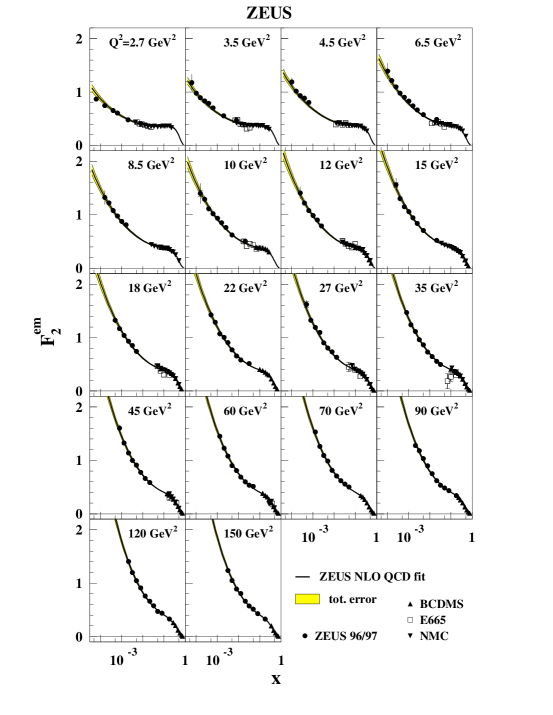
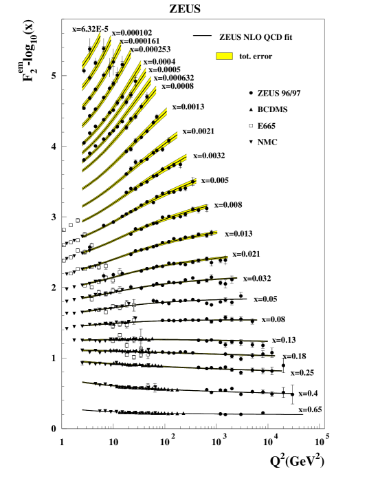
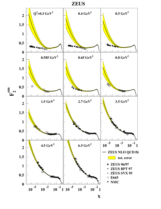
The ZEUS-S fit, with , is shown in Figs. 1-4. In Fig. 1, the fit prediction for is shown compared to the ZEUS and proton fixed-target data as a function of at low . In Fig. 2, this comparison is made as a function of for values in the range . For the fixed-target data, only the -exchange process contributes to , whereas, at high-, there are also contributions from exchange and interference. Thus, for comparability with the fixed-target results, the ZEUS data shown in these figures represent only that part of due to exchange, as denoted by the symbol . The fit gives an excellent description of the data.
The goodness of fit cannot be judged from the calculated from statistical and uncorrelated systematic errors alone. Re-evaluating the for the parameters resulting from the ZEUS-S fit by adding the statistical, uncorrelated and correlated systematic errors in quadrature gives a total per data point of 0.95 for 1263 data points and 11 free parameters. The per data point for individual data sets calculated in the same way are listed in Table 1.
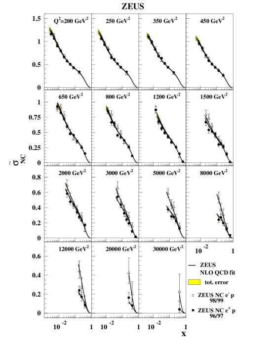
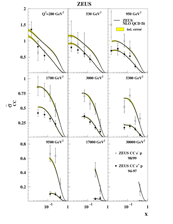
In Fig. 3, the fit is compared to the ZEUS high- neutral current data. This figure also shows predictions for the neutral current data [21], which were not included in the fit. The charged current [19] and [20] data (which were also not included in the fit) are compared to the fit prediction in Fig. 4. These high- data are very well described by the fit.
4.2 Parton distribution functions and
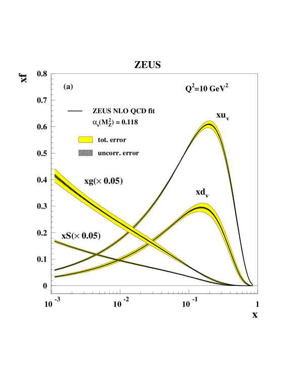
The PDF parameters extracted from the ZEUS-S fit at are given in Table 2 and the corresponding parton distributions at are shown in Fig. 5(a). The precision of these distributions is considerably improved in comparison to a fit [10] using earlier ZEUS data. The total error band is dominated by systematic uncertainties. In Fig. 5(b), the ZEUS parton distributions are compared to the latest distributions from MRST [5] and CTEQ [6]. The differences between these sets of parton distributions are compatible with the size of the error bands on the ZEUS parton distributions.
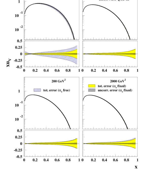
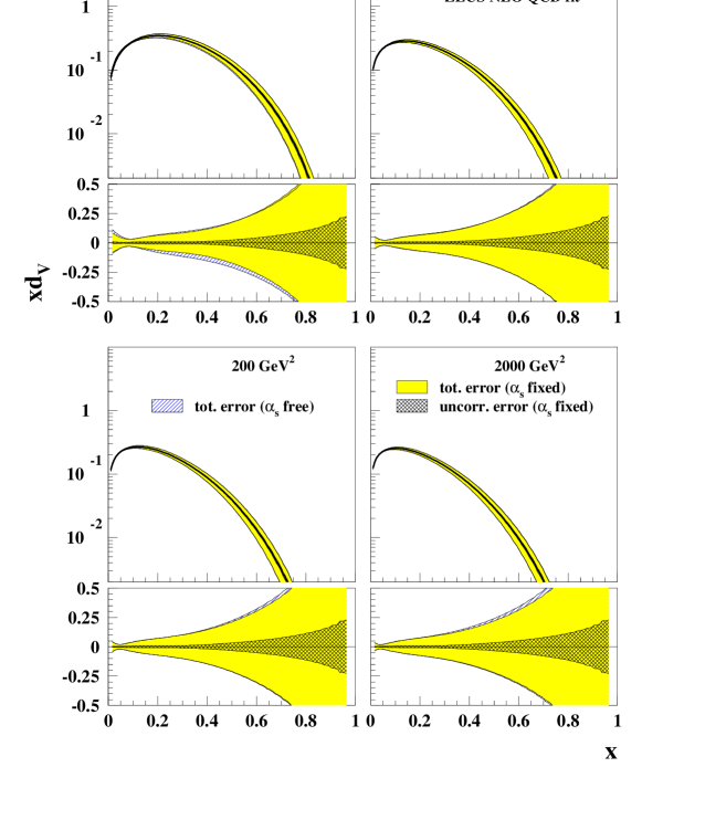
The PDFs extracted from the ZEUS-S fit are now considered in more detail. In these distributions, the contribution to the error bands coming from variation of will be indicated in addition to the contributions of correlated and uncorrelated experimental uncertainties. This additional uncertainty has been taken into account with full correlations by allowing to be a parameter of the ZEUS- fit (see Section 4.3).
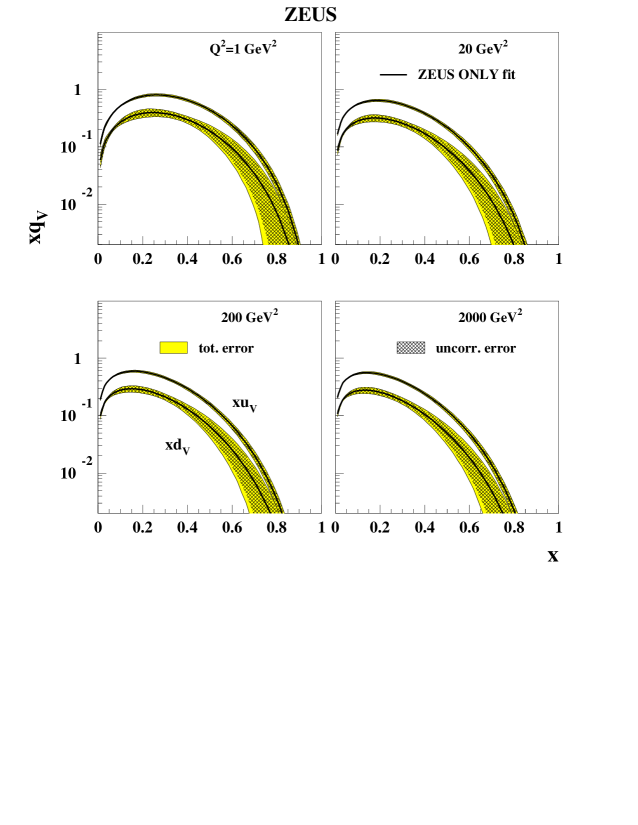
The valence distributions and extracted from the fit are shown for several different values in Figs. 6 and 7. The abscissa is linear and the ordinate logarithmic to illustrate the high- behaviour of these valence distributions, where they are constrained by the fixed-target data. The distributions for are obtained by backward extrapolation. The uncertainty is shown beneath each distribution in terms of the fractional differences from the central value. The -valence distribution is much better determined than the -valence distribution, since structure-function data from fixed-target experiments are dominated by the quark.
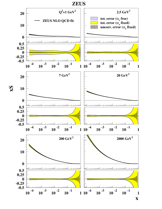
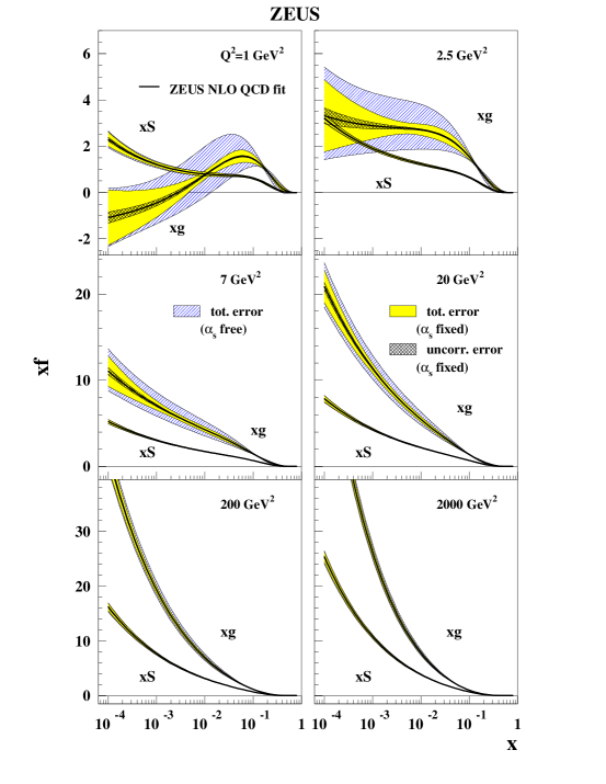
The extracted sea distribution and its uncertainty is shown for several values in Fig. 8. The uncertainty in these distributions is less than for and , but considerable uncertainty remains for . The sea distribution rises at small , even at .
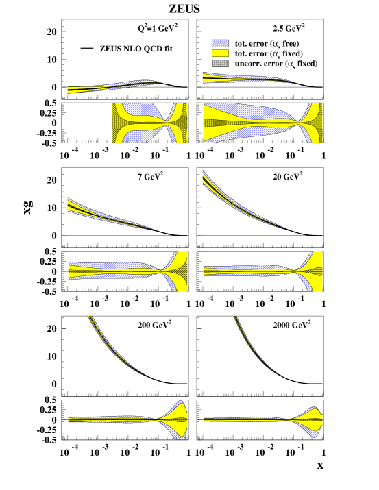
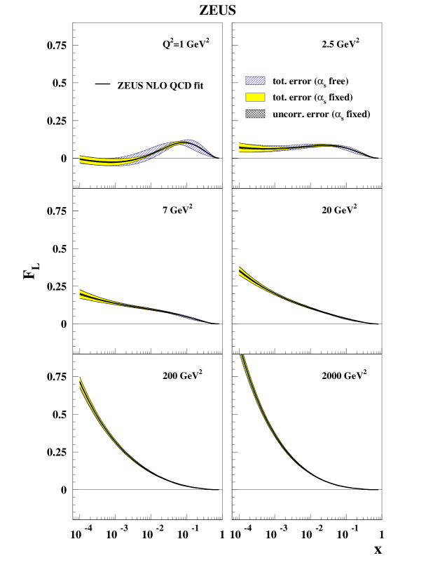
The corresponding gluon distribution and its uncertainty is shown for several values in Fig. 9. The general shape of the error bands, with a narrowing at , is a consequence of the momentum sum rule. The gluon distribution is determined to within for and ; and its uncertainty decreases as increases. Considerable uncertainty remains for . The distribution rises steeply at low for ; however, at lower , the low- gluon shape is flatter. When the fit is extrapolated back to , the shape becomes valence-like and tends to become negative at the lowest , although remaining consistent with zero.
The shapes of the gluon and the sea distributions are compared in Fig. 10. For , the gluon density becomes much larger than the sea density, but for lower the sea density continues to rise at low , whereas the gluon density is suppressed. The present analysis shows this contrasting behaviour of the low-, low- gluon and sea distributions even more clearly than the previous study of earlier ZEUS data [17].
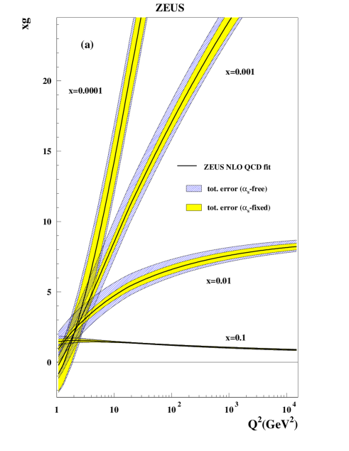
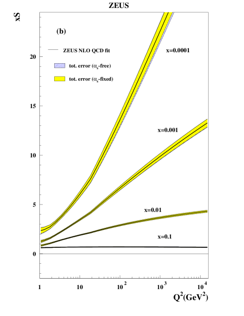
It is also interesting to compare the behaviour of the gluon and the sea NLO densities as a function of for fixed values. This is shown in Fig. 11. The scaling violation of the gluon distribution at small is striking, reflecting the singular behaviour of the and splitting functions as .
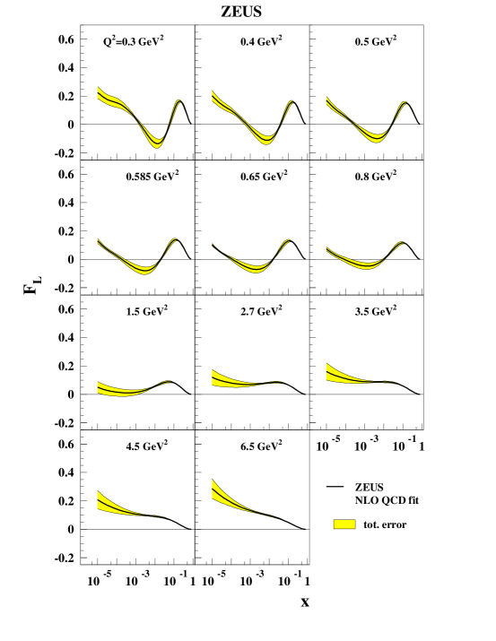
The tendency of the gluon distribution to become negative at low and low could be a signal that NLO QCD is inadequate in this kinematic region. However, the only physical requirement is that the structure functions calculated from the parton distributions are positive. Thus it is important to investigate the fit prediction for , the structure function most closely related to the gluon [84]. This is shown in Fig. 12. It exhibits similar features to the gluon. This will be discussed further in Section 6.
4.3 The extraction of
In the evolution of singlet quark distributions at intermediate (), the value of and the gluon shape are strongly correlated through the DGLAP equations, since an increase in can be compensated by a harder gluon distribution. This has restricted the precision of determinations of from NLO DGLAP fits to DIS data in the past. However, at small () this correlation is weakened, since the gluon then drives the behaviour of as well as that of . Thus, precision low- data can be used to make a simultaneous fit for and the PDF parameters. In the ZEUS- fit, was left free, leading to
| (3) |
where the three uncertainties arise from the following: statistical and other uncorrelated sources; correlated systematic sources from all the contributing experiments except that from their normalisations; the contribution from the latter normalisations.
The difference between this value of and the value used in the ZEUS-S fit does not produce any significant shifts in the PDF parameters as compared to those determined in the ZEUS-S fit. However, the correlation between and the PDF parameters does increase their experimental uncertainties, particularly that of the gluon, as illustrated in Figs. 6-12.
4.4 Model uncertainties
Sources of model uncertainty within the theoretical framework of leading-twist NLO QCD are now considered. The sensitivity of the results to the variation of input assumptions has been quantified in terms of the resulting variation in , since it is the most sensitive parameter.
Table 3 summarizes the effect of varying the value of , and the minimum , and (, , ) of data entering the ZEUS- fit, in terms of the shift in the central value of . These variations produce only a small model uncertainty in and in the PDF parameters.
It is also necessary to consider varying the form of the input PDF parameterisations. Variation in the gluon parameterisation produces the most significant effects since it is least well known. Allowing the high- gluon to take a more complex form, with , resulted in a shift of . Extending the form of the parameterisation from to for both the gluon and the other parton distributions resulted in a shift of . Allowing to be free for the valence distributions had no further effect on the value of . Finally, information from Tevatron high- jet production [85, 86] was used to constrain the high- gluon [5]. The corresponding shift in the central value of was and the shape of the gluon was shifted to be harder at high . However, these shifts are well within the error estimates for both and the gluon PDF parameters.
A further significant choice is that of the heavy-quark production scheme. Repeating the fit using the FFN scheme or the ZMVFN scheme produced shifts of . Variation of the heavy-quark mass within the FFN and TRVFN schemes produced smaller shifts. The choice of the heavy-quark scheme also affects the shape of the gluon, such that the FFN scheme gluon is steeper at small than the ZMVFN scheme gluon, with the TRVFN gluon in between. The size of these shifts is well within the error estimates of the gluon PDF parameters.
Thus, the total model uncertainty on is considerably smaller than the errors from correlated systematic and normalisation uncertainties and leads to
4.5 Uncertainties in the theoretical framework
While the uncertainty within the theoretical framework of leading-twist NLOQCD is rather well defined, it is much more difficult to decide on the uncertainty caused by reasonable variations in the framework. In this Section, two variations on the framework are estimated; the treatment of higher-twist terms and the choice of the renormalisation and factorisation scales, which gives an estimate of the importance of the higher-order terms in the pQCD expansion.
The analysis was performed at leading twist and accordingly a hard cut was made to remove the region where higher-twist effects are known to be important. In order to evaluate if there are residual effects of higher twist at such large , this cut was lowered to and the SLAC data [87] were included111Note that the for these data must be calculated by adding statistical and systematic errors in quadrature, since information on correlated point-to-point systematic uncertainties is not available.. A fit in which the leading-twist predictions for were modified by a factor was then performed, where , , are parameters determined in ten bins of [88]. This modification was not intended to provide a thorough study of the higher-twist effects themselves, but only as an estimate of the uncertainty introduced by neglecting them. Hence, a simple form of the higher-twist contribution was used, in which was not modified and the higher-twist terms for deuterium and proton targets were assumed to be the same. The contribution of higher twist was found to be negligible for , small and negative for and large and positive for , where target-mass effects are important. Having determined the parameters in this fit, these parameters were fixed and a fit was performed with the usual hard cut (excluding SLAC data). This produced a shift of .
Variation of the renormalisation and factorisation scales used in the fit was also considered. The choice of for these scales is conventional in the inclusive DIS process, and their variation is used as a crude way of estimating the importance of higher-order terms [89, 90, 91, 92]. These scales were varied from , independently and simultaneously. This produced shifts , mostly from the change in renormalisation scale. The result of making larger scale changes, such as , is not presented because such large scale changes produce fits with much larger , which are unacceptable according to the ‘hypothesis testing’ criterion (see Appendix). It is unclear that such arbitrary scale changes give any reasonable estimate of the importance of higher-order terms [5]. Several groups [93, 94, 95] have compared NLO and approximate NNLO analyses. The change in obtained in these studies is in the range .
The uncertainties discussed in this Section are rather large. However, since these investigations are far from exhaustive and given the difficulties in defining a reasonable variation in the theoretical framework, they are not included in the uncertainties quoted on the final value of .
5 Parton densities from ZEUS data alone
The fit using ZEUS data only (ZEUS-O) uses the charged current data [19] and the neutral and charged current data [21, 20] in addition to the neutral current data [7]. These high- data are very well described by the ZEUS-S fit, as illustrated in Figs. 3 and 4. However, in the ZEUS-O fit these additional data sets were used instead of the fixed-target data to constrain the valence distributions. Note that the for these additional data sets must be calculated by adding statistical and systematic errors in quadrature. The correlated point-to-point systematic uncertainties are small compared to the statistical uncertainties for these data sets. Since the exclusion of the fixed-target data leaves no constraint on the flavour content of the sea, the value of for the distribution was fixed to the value determined in the ZEUS-S fit. The value was fixed; all other parameters were varied as usual.
The gluon and the sea distributions extracted from the ZEUS-O fit are shown in Fig. 13. Comparing this figure to Fig. 10, it is clear that the gluon and sea densities are mainly determined by the ZEUS data for . The ZEUS-O fit gives almost as good a determination of these distributions as the ZEUS-S fit over most of the plane used in the fit.
The valence distributions extracted from the ZEUS-O fit are shown in Fig. 14. They are determined to a precision about a factor of two worse than in the ZEUS-S fit. The -valence distribution is well determined; however, the -valence distribution is much more poorly determined. In the ZEUS-O fit, the -valence distribution is determined by the high- charged current data. In contrast in the ZEUS-S fit the -valence distribution is determined by the deuterium fixed-target data. Recently it has been suggested that such measurements are subject to significant uncertainty from deuteron binding corrections [96, 97, 98, 99, 100]. The ZEUS-O extraction does not suffer this uncertainty. It produces a larger -valence distribution at high- than the ZEUS-S fit, as can be seen by comparison with Fig. 7, but there is no disagreement within the limited statistical precision of the current high- data.
6 The transition to very low
The ZEUS-S and ZEUS- fits and the NLO QCD fits of MRST [30, 31, 55, 5] and CTEQ [64, 65, 6] give good descriptions of data down to values of . For such fits to be valid, it is necessary to assume that the formalism is valid even for low [101], where is large and perturbation theory may break down, as well as for very low , where resummation terms should become important [90, 91, 92, 102, 103]. High-density and non-perturbative effects [104] are also neglected. To investigate if there is a low- limit to the applicability of the NLO QCD DGLAP formalism, the ZEUS-S fit was extrapolated into the region covered by ZEUS shifted-vertex (SVX) data [17] and the precise ZEUS beam-pipe-tracker (BPT) data [22].
In Fig. 15, the ZEUS 96/97 data and the SVX and BPT data are shown at very low compared to the predictions of the ZEUS-S fit. The increased precision of the new data, both at intermediate and at very low , lead to a firmer conclusion than in the previous study [17]. The ZEUS-S fit is able to describe the data down to , but exceeds the data at , and clearly fails for , even when the conservative error bands on the fit due to the correlated systematic uncertainties are included. Thus, the NLO DGLAP formalism describes the extreme steepness of the ZEUS data at intermediate () but is unable to accommodate the rapid transition to a flatter behaviour at . The ZEUS-S fit predictions for for very low- values are also shown in Fig. 16. The significantly negative values of for are a further indication that the NLO DGLAP formalism is not applicable.
7 Summary and conclusions
The NLO DGLAP QCD formalism has been used to fit the 1996-1997 ZEUS data and fixed-target data in the kinematic region , and . Full account has been taken of correlated experimental systematic uncertainties. A good description of the structure function and reduced cross section over the range from to has been obtained.
The parton distribution functions for the and valence quarks, the gluon and the total sea have been determined and the results are compatible with those of MRST2001 and CTEQ6. The ZEUS data are crucial in determining the gluon and the sea distributions and a fit to ZEUS data alone shows that these data also constrain the valence-quark distributions. The new high-precision data allow a greatly improved determination of the gluon and sea distributions.
At , the fit predicts that the sea distribution is still rising at small , whereas the gluon distribution is suppressed. The fit is unable to describe the precise ZEUS BPT data for and also predicts unphysical negative values for in this region. Hence the use of the NLO QCD DGLAP formalism at is questionable.
The ZEUS data at low have been used to extract the value of in a simultaneous fit to and the shapes of the input parton distributions, including correlations between them, giving
Uncertainties in the leading twist NLO QCD framework are also significant but cannot be easily quantified.
The statistical accuracy of the ZEUS data is now sufficient to give a very good determination of the sea and gluon PDFs. With the full HERA-II data sample, it will be possible to extend this analysis to give an accurate determination of all proton PDFs within a single experiment.
Appendix
A. Comparison of different ways of calculating
The used in this analysis is defined in Eq. (1) and the modification of the theoretical predictions to account for correlated systematic uncertainties is given in Eq. (2). The has been evaluated with the systematic-offset parameters set to zero, , with the consequence that the fitted theoretical predictions are as close as possible to the central values of the published data. The offset parameters were then allowed to vary in the evaluation of the error to account for correlation between systematic-uncertainty parameters and theoretical parameters, as described in Section 3.3.
This method is referred to as the ‘offset method’, since it is approximately equivalent to offsetting each systematic parameter by , performing a new fit for each of these variations and adding in quadrature the resulting deviations of the theoretical parameters from their central values [16]. This procedure does not assume that the systematic errors are Gaussian distributed. This is a conservative method of error estimation as compared to the Hessian methods described below [11, 16].
An alternative procedure would be to allow the systematic uncertainty parameters to vary in the main fit when determining the values of the theoretical parameters. This was the procedure adopted by a recent H1 analysis [8], in which only H1 and BCDMS data were considered. This method is referred to as ‘Hessian method 1’. The errors on the theoretical parameters are calculated from the inverse of a single Hessian matrix which expresses the variation of with respect to both theoretical and systematic offset parameters. Effectively, the theoretical prediction is not fitted to the central values of the published experimental data, but allows these data points to move collectively according to their correlated systematic uncertainties. The theoretical prediction determines the optimal settings for correlated systematic shifts of experimental data points such that the most consistent fit to all data sets is obtained. Thus the fit correlates the systematic shifts in one experiment to those in another experiment.
Hessian method 1 becomes a cumbersome procedure when the number of sources of systematic uncertainty is large, as in the present global DIS analysis. Recently the CTEQ [13, 14] collaboration has given an elegant analytical method for performing the minimization with respect to systematic-uncertainty parameters. This gives a new formulation of the :
where
and
such that the uncorrelated and correlated systematic contributions to the can be evaluated separately. This method is referred to as ‘Hessian method 2’.
These two Hessian methods have been compared for the ZEUS-O fit, in which the systematic uncertainties are well understood. The results are very similar, as expected if the systematic uncertainties are Gaussian and the values are standard deviations. However, if data sets from different experiments are used in the fit, the results of these two Hessian methods are only similar if normalisation uncertainties are not included.
The offset method has been compared to Hessian method 2 by performing the ZEUS- fit to global DIS data using Hessian method 2 to calculate the . Normalisation uncertainties were excluded and was included as one of the theoretical parameters. This fit yields , where the error represents the total experimental uncertainty from correlated and uncorrelated sources, excluding normalisation uncertainties. Thus this value should be compared with , evaluated using the offset method, also excluding normalisation uncertainties (see Eq. 3). Hessian method 2 gives a much reduced error estimate for both and the PDF parameters. The value of is shifted from that obtained by the offset method. The PDF parameters are not affected as strongly; their values are shifted by amounts which are well within the error estimates quoted for the offset method.
To compare the of the fits performed using the offset method and Hessian method 2, it is necessary to use a common method of calculation. Table 4 presents the for the theoretical parameters obtained using each of these methods, re-evaluated by adding statistical and systematic errors in quadrature. For both methods, has been included among the theoretical parameters and normalisation uncertainties have not been included among the systematic parameters. The total increase of for Hessian method 2 as compared to the offset method is . Thus the results of Hessian method 2 represent a fit with an unacceptably large value of when judged in this conventional way.
B. Parameter estimation and hypothesis testing
To appreciate the signficance of the difference in between various fits, the distinction between the changes appropriate for parameter estimation and for hypothesis testing should be considered. Assuming that the experimental uncertainties that contribute have Gaussian distributions, errors on theoretical parameters that are fitted within a fixed theoretical framework are derived from the criterion for ‘parameter estimation’ . However, the goodness of fit of a theoretical hypothesis is judged on the ‘hypothesis testing’ criterion, such that its should be approximately in the range , where is the number of degrees of freedom.
Fitting DIS data for PDF parameters and is not a clean situation of either parameter estimation or hypothesis testing, nor are the contributing experimental uncertainties always Gaussian distributed. Within the theoretical framework of leading-twist NLO QCD, many model inputs, such as the form of the PDF parameterisations, the values of cuts, the value of , the data sets used in the fit, etc. can be varied. These represent different hypotheses and they are accepted provided the fit falls within the hypothesis-testing criterion. The theoretical parameters obtained for these different model hypotheses can differ from those obtained in the standard fit by more than their errors as evaluated using the parameter-estimation criterion. In this case, the model error on the parameters can exceed the estimate of the total experimental error. This does not happen for the offset method, in which the uncorrelated experimental errors evaluated by the parameter-estimation criterion are augmented by the contribution of the correlated experimental systematic uncertainties, as explained in Section 3.3. The shifts in theoretical parameter values for the different model hypotheses were found to be well within the total experimental error estimates222Note that this is true whether or not normalisation uncertainties are included in these estimates.. However, this is no longer the case when the fit is performed using Hessian method 2.
The CTEQ collaboration [14, 6] have considered this problem. They consider that is not a reasonable tolerance on a global fit to approximately data points from diverse sources, with theoretical and model uncertainties that are hard to quantify and experimental uncertainties that may not be Gaussian distributed. They have tried to formulate criteria for a more reasonable setting of the tolerance , such that becomes the variation on the basis of which errors on parameters are calculated. In setting this tolerance they have considered that all of the current world data sets must be acceptable and compatible at some level. The level of tolerance they suggest is . The error estimates of the present fit have been re-evaluated using Hessian method 2 for various values of the tolerance. For the errors on the PDF parameters and on are very similar to those of the offset method performed under the same conditions 333This remains the case when normalisation uncertainties are introduced into each of these methods. . For example, the result is obtained. Note that the value is similar to the hypothesis-testing tolerance for the fits.
Thus the offset method and the Hessian method with a modified tolerance give similar error estimates. In choosing between these methods, there are some additional considerations. In the Hessian method 2, it is necessary to check that data points are not shifted far outside their uncertainties. When the ZEUS- and the ZEUS-S fit are done by Hessian method 2 some of the systematic shifts for the ten classes of systematic uncertainty of the ZEUS data move by standard deviations. No single kinematic region responsible for these shifts could be identified. Whereas these shifts are not very large, it is significant that they differ from the systematic shifts to ZEUS data determined in the CTEQ fit [6]. They also differ from those determined in the ZEUS-O fit done by Hessian method 2. Making different model assumptions in the fits also produces somewhat different systematic shifts. It seems unreasonable to let variations in the model, or the choice of data included in the fit, change the best estimate of the central value of the data points.
In summary, the offset method has been selected for several reasons. First, its fit results make theoretical predictions that are as close to the central values of the published data points as possible. The selection of data sets included in the fit or superficial changes to the model do not change the best estimate of the central value of the data points. Secondly, it is approximately equivalent to a method that does not assume that experimental systematic uncertainties are Gaussian distributed. Thirdly, its results produce an acceptable when re-evaluated conventionally by adding systematic and statistical errors in quadrature. Fourthly, its error estimates take account of the fact that the purpose is to estimate errors on the PDF parameters and within a general theoretical framework not specific to particular model choices. Quantitatively, the error estimates of the offset method correspond to those that would be obtained using the more generous tolerance in the more statistically powerful Hessian methods.
Acknowledgements
We would like to thank R.S. Thorne and R.G. Roberts for useful discussions. The experiment was made possible by the skill and dedication of the HERA machine group who ran HERA most efficiently during the years when the data used in this paper were collected. The realisation and continuing operation of the ZEUS detector has been and is made possible by the inventiveness and continuing hard work of many people not listed as authors. Their contributions are acknowledged with great appreciation. The support and encouragement of the DESY directorate continues to be invaluable for the successful operation of the ZEUS collaboration.
We acknowledge support by the following: the Natural Sciences and Engineering Research Council of Canada (NSERC); the German Federal Ministry for Education and Research (BMBF), under contract numbers HZ1GUA 2, HZ1GUB 0, HZ1PDA 5, HZ1VFA 5; the MINERVA Gesellschaft für Forschung GmbH; the Israel Science Foundation, the U.S.-Israel Binational Science Foundation; the Israel Ministry of Science and the Benozyio Center for High Energy Physics; the German-Israeli Foundation, the Israel Science Foundation; the Italian National Institute for Nuclear Physics (INFN); the Japanese Ministry of Education, Science and Culture (the Monbusho) and its grants for Scientific Research; the Korean Ministry of Education and Korea Science and Engineering Foundation; the Netherlands Foundation for Research on Matter (FOM); the Polish State Committee for Scientific Research, under grant numbers 620/E-77/SPUB-M/DESY/P-03/DZ 247/2000-2002; the Fund for Fundamental Research of Russian Ministry for Science and Education; the Spanish Ministry of Education and Science through funds provided by CICYT; the Particle Physics and Astronomy Research Council, UK; the US Department of Energy; the US National Science Foundation; the Polish State Committee for Scientific Research under grant numbers 112/E-356/SPUB-M/DESY/P-03/DZ 301/2000-2002, 2 P03B 13922, 115/E-343/SPUB-M/DESY/P-03/DZ 121/2001-2002, 2 P03B 07022. J. Rautenberg was supported by the German-Israeli Foundation, contract number I-523-13.7/97; D.S. Bailey and N.H. Brook are PPARC Advanced fellows; E. Rodrigues and R. Gonçalo were supported by the Portuguese Foundation for Science and Technology; J. Szuba was partly supported by the Israel Science Foundation and the Israel Ministry of Science; A. Kotański was supported by the Polish State Committee for Scientific Research, grant number 2 P03B 09322; J.H. Loizides was supported by Argonne National Laboratory, USA; R. Ciesielski was supported by the Polish State Committee for Scientific Research, grant number 2 P03B 07222; T. Tymieniecka and A. Ukleja were supported by German Federal Ministry for Education and Research (BMBF), POL 01/043; L.K. Gladilin was partly supported by University of Wisconsin via the U.S.-Israel Binational Science Foundation.
100
References
- [1] V.N. Gribov and L.N. Lipatov, Sov. J. Nucl. Phys. 15, 438 (1972)
- [2] L.N. Lipatov, Sov. J. Nucl. Phys. 20, 94 (1975)
- [3] G. Altarelli and G. Parisi, Nucl. Phys. B 126, 298 (1977)
- [4] Yu.L. Dokshitzer, Sov. Phys. JETP 46, 641 (1977)
- [5] A.D. Martin et al., Eur. Phys. J. C 23, 73 (2002)
- [6] J. Pumplin et al., JHEP 0207 012 (2002)
- [7] ZEUS Coll., S. Chekanov et al., Eur. Phys. J. C 21, 443 (2001)
- [8] H1 Coll., C. Adloff et al., Eur. Phys. J. C 21, 33 (2001)
- [9] W.T. Giele and S.A. Keller, Phys. Rev. D 58, 094023 (1998)
- [10] M. Botje, Eur. Phys. J. C 14, 285 (2000)
- [11] S.I. Alekhin, Preprint hep-ex/0005042, 2000
- [12] CTEQ Coll., D. Stump et al., in Proc. Int. Workshop on Deep-Inelastic Scattering (DIS2000), Liverpool, p. 159. World Scientific, Singapore, 2000
- [13] CTEQ Coll., D. Stump et al., Phys. Rev. D 65, 014012 (2001)
- [14] CTEQ Coll., J. Pumplin et al., Phys. Rev. D 65, 014013 (2001)
- [15] W.T. Giele, S.A. Keller and D.A. Kosover, Preprint hep-ph/0104052, 2001
- [16] M. Botje, J. Phys. G 28, 779 (2002)
- [17] ZEUS Coll., J. Breitweg et al., Eur. Phys. J. C 7, 609 (1999)
- [18] Particle Data Group, D.E. Groom et al., Eur. Phys. J. C15, 1 (2000)
- [19] ZEUS Coll., J. Breitweg et al., Eur. Phys. J. C 12, 411 (2000)
- [20] ZEUS Coll., S. Chekanov et al., Phys. Lett. B 539, 197 (2002)
- [21] ZEUS Coll., S. Chekanov et al., Preprint DESY-02-113, DESY, 2002, submitted to Eur.Phys.J
- [22] ZEUS Coll., J. Breitweg et al., Phys. Lett. B 487, 53 (2000)
- [23] ZEUS Coll., J. Breitweg et al., Phys. Lett. B 407, 432 (1997)
- [24] R.G. Roberts, The Structure of the Proton. Cambridge University Press, 1990
- [25] A. De Rújula et al., Phys. Rev. D 10, 1649 (1974)
- [26] ZEUS Coll., M. Derrick et al., Phys. Lett. B 316, 412 (1993)
- [27] H1 Coll., I. Abt et al., Nucl. Phys. B 407, 515 (1993)
- [28] ZEUS Coll., M. Derrick et al., Z. Phys. C 72, 399 (1996)
- [29] H1 Coll., S. Aid et al., Nucl. Phys. B 470, 3 (1996)
- [30] A.D. Martin, R.G. Roberts and W.J. Stirling, Phys. Lett. B 387, 419 (1996)
- [31] A.D. Martin et al., Eur. Phys. J. C 4, 463 (1998)
- [32] L.N. Lipatov, Sov. J. Nucl. Phys. 23, 338 (1976)
- [33] E.A. Kuraev, L.N. Lipatov and V.S. Fadin, Sov. Phys. JETP 45, 199 (1977)
- [34] Ya.Ya. Balitskiĭ and L.N. Lipatov, Sov. J. Nucl. Phys. 28, 822 (1978)
- [35] L.N. Lipatov, Sov. J. Nucl. Phys. 63, 904 (1980)
- [36] V.S. Fadin and L.N. Lipatov, Phys. Lett. B 429, 127 (1998)
- [37] G. Camici and M. Ciafaloni, Phys. Lett. B 430, 349 (1998)
- [38] A. Mueller, Preprint CU-TP-1035 (hep-ph/0111244), Columbia Univ., 2001
- [39] BCDMS Coll., A.C. Benvenuti et al., Phys. Lett. B 223, 485 (1989)
- [40] NMC Coll., M. Arneodo et al., Nucl. Phys. B 483, 3 (1997)
- [41] E665 Coll., M.R. Adams et al., Phys. Rev. D 54, 3006 (1996)
- [42] NMC Coll., M. Arneodo et al., Nucl. Phys. B 487, 3 (1997)
- [43] W.G. Seligman et al., Phys. Rev. Lett. 79 (1997)
- [44] A. Bodek, in Proc. Int. Workshop on Deep-Inelastic Scattering (DIS2000), Liverpool, p. 103. World Scientific, Singapore, 2000
- [45] A. Bodek, in Proc. Int. Conf. on High Energy Physics (ICHEP2000), Osaka, Japan, p. 441. World Scientific, Singapore, 2000
- [46] J. Gomez et al., Phys. Rev. D 49, 4348 (1994)
- [47] H. Georgi and H.D. Politzer, Phys. Rev. D 14, 1829 (1976)
- [48] M. Virchaux and A. Milsztajn, Phys. Lett. B 274, 221 (1992)
- [49] G. Gurci, W. Furmanski and R. Petronzio, Nucl. Phys. B 175, 27 (1980)
- [50] W. Furmanski and R. Petronzio, Phys. Lett. B 97, 437 (1980)
- [51] W. Furmanski and R. Petronzio, Z. Phys. C 11, 293 (1982)
- [52] CCFR Coll., A.O. Bazarko et al., Z. Phys. C65, 189 (1995)
- [53] FNAL E866/NuSea Coll., E.A. Hawker et al., Phys. Rev. Lett. 80, 3715 (1998)
- [54] A.D. Martin et al., Eur. Phys. J. C 14, 133 (2000)
- [55] A.D. Martin et al., Nucl. Phys. Proc. Suppl. 79, 105 (1999)
- [56] P. Amaudruz et al., Phys. Lett. B 295, 159 (1992)
- [57] P. Amaudruz et al., Phys. Rev. Lett. 66, 2712 (1991)
- [58] M. Botje, QCDNUM version 16.12 (unpublished)
- [59] A.D. Martin, R.G. Roberts and W.J. Stirling, Phys. Rev. D 47, 867 (1993)
- [60] A.D. Martin, R.G. Roberts and W.J. Stirling, Phys. Rev. D 50, 6734 (1994)
- [61] A.D. Martin, R.G. Roberts and W.J. Stirling, Phys. Lett. B 354, 155 (1995)
- [62] CTEQ Coll., J. Botts et al., Phys. Lett. B 304, 159 (1995)
- [63] CTEQ Coll., H.L. Lai et al., Phys. Rev. D 51, 4763 (1995)
- [64] CTEQ Coll., H.L. Lai et al., Phys. Rev. D 55, 1280 (1997)
- [65] CTEQ Coll., H.L. Lai et al., Eur. Phys. J. C 12, 375 (2000)
- [66] M. Glück, E. Reya and A. Vogt, Z. Phys. C 67, 433 (1995)
- [67] M. Gluck, E. Reya and M. Stratmann, Nucl. Phys. B 422, 37 (1994)
- [68] M. Glück, E. Reya and A. Vogt, Eur. Phys. J. C 5, 461 (1998)
- [69] H.L Lai and W.K. Tung, Z. Phys. C 74, 463 (1997)
- [70] A.D. Martin et al., Eur. Phys. J. C 2, 287 (1998)
- [71] M.A.G. Aivazis et al., Phys. Rev. D 50, 3102 (1994)
- [72] M. Buza et al., Eur. Phys. J. C 1, 301 (1998)
- [73] F.I. Olness and R.J. Scalise, Phys. Rev. D 57, 241 (1998)
- [74] M. Kramer et al., Phys. Rev. D 62, 096007 (2000)
- [75] A. Chuvakin, J. Smith amd W.L. van Neerven, Phys. Rev. D 61, 096004 (2000)
- [76] A. Chuvakin et al., Eur. Phys. J. C 18, 547 (2001)
- [77] R.S. Thorne, J. Phys. G 25, 1307 (1999)
- [78] R.S. Thorne and R.G. Roberts, Phys. Lett. B 421, 303 (1998)
- [79] R.S. Thorne and R.G. Roberts, Phys. Rev. D 57, 6871 (1998)
- [80] R.S. Thorne and R.G. Roberts, Eur. Phys. J. C 19, 339 (2001)
- [81] F. James, Minuit v94.1, CERN Program Library Long Writeup D506 (unpublished), available on http://wwwinfo.cern.ch/asdoc/minuit/minmain.html
- [82] C. Pascaud and F. Zomer, Preprint LAL-95-05, LAL, 1995
- [83] M. Virchaux and A. Milsztajn, Preprint DPhPE-90-07, DPhPe, 1990
- [84] A.M. Cooper-Sarkar et al., Z. Phys. C 39, 281 (1988)
- [85] DØ Coll., B. Abbott et al., Phys. Rev. Lett. 86, 1707 (2000)
- [86] CDF Coll., T. Affolder et al., Phys. Rev. D 64, 012001 (2001)
- [87] L.W. Whitlow et al., Phys. Lett. B 282, 475 (1992)
- [88] A.D. Martin et al., Phys. Lett. B 443, 301 (1998)
- [89] A.D. Martin et al., Eur. Phys. J. C 18, 117 (2000)
- [90] R.S. Thorne, Phys. Rev. D 64, 074005 (2001)
- [91] A.M. Cooper-Sarkar, in Proc. Int. Symposium on Multiparticle Dynamics (ISMD2000), Balaton, Hungary, p. 73. World Scientific, Singapore, 2001
- [92] R.S. Thorne, Phys. Lett. B 474, 372 (2000)
- [93] A.D. Martin et al., Phys. Lett. B 531, 216 (2002)
- [94] S.I. Alekhin, Phys. Lett. B 519, 57 (2001)
- [95] J. Santiago and F.J. Yndurain, Nucl. Phys. B 611, 447 (2001)
- [96] W. Melnitchouk and A.W. Thomas, Phys. Lett. B 377, 11 (1996)
- [97] W. Melnitchouk and J.C. Peng, Phys. Lett. B 400, 220 (1997)
- [98] U.K. Yang and A. Bodek, Phys. Rev. Lett. 82, 2467 (1999)
- [99] U.K. Yang and A. Bodek, Eur. Phys. J. C 13, 241 (2000)
- [100] U.K. Yang and A. Bodek, Phys. Rev. Lett. 84, 5456 (2000)
- [101] E. Ruiz Arriola, Nucl. Phys. A 641, 461 (1999)
- [102] G. Altarelli, S. Forte and R.D. Ball, Nucl. Phys. B 599, 383 (2001)
- [103] G. Altarelli, S. Forte and R.D. Ball, Nucl. Phys. B 621, 359 (2002)
- [104] A.M. Cooper-Sarkar, R.C.E. Devenish and A. De Roeck, Int. J. Mod. Phys. A 13, 3385 (1998)
| Experiment | Number of data | per | Number of correlated | Number of normalisation |
|---|---|---|---|---|
| points | data point | systematic uncertainties | uncertainties | |
| ZEUS96/97 [7] | 242 | 0.85 | 10 | 2 |
| BCDMS p [39] | 305 | 0.94 | 5 | 5 |
| NMC p [40] | 218 | 1.21 | 12 | 4 |
| NMC D [40] | 218 | 0.92 | ||
| NMC D/p [42] | 129 | 0.94 | 5 | 0 |
| E665 D [41] | 47 | 0.94 | 7 | 2 |
| E665 p [41] | 47 | 1.16 | 1 | |
| CCFRxF3 [43] | 57 | 0.40 | 18 | 0 |
| () | ||||
| ( | ||||
| () | ||||
| () |
| Nominal value | New value | |
|---|---|---|
| +0.0008 | ||
| -0.0004 | ||
| -0.0007 | ||
| -0.0005 | ||
| -0.0005 |
| Experiment | Data points | /data point | /data point |
|---|---|---|---|
| Hessian method 2 | Offset method | ||
| ZEUS96/97 | 242 | 1.37 | 0.83 |
| BCDMS p | 305 | 0.95 | 0.89 |
| NMC p | 218 | 1.50 | 1.26 |
| NMC D | 218 | 1.15 | 0.96 |
| NMC D/p | 129 | 0.97 | 0.93 |
| E665 D | 47 | 0.97 | 0.94 |
| E665 p | 47 | 1.17 | 1.16 |
| CCFRxF3 | 57 | 0.99 | 0.39 |