AN UNFOLDING METHOD FOR HIGH ENERGY PHYSICS EXPERIMENTS

Abstract

Finite detector resolution and limited acceptance require to apply unfolding methods in high energy physics experiments. Information on the detector resolution is usually given by a set of Monte Carlo events. Based on the experience with a widely used unfolding program (RUN) a modified method has been developed.

The first step of the method is a maximum likelihood fit of the Monte Carlo distributions to the measured distribution in one, two or three dimensions; the finite statistic of the Monte Carlo events is taken into account by the use of Barlows method with a new method of solution. A clustering method is used before to combine bins in sparsely populated areas. In the second step a regularization is applied to the solution, which introduces only a small bias. The regularization parameter is determined from the data after a diagonalization and rotation procedure.

1 THE UNFOLDING PROBLEM

A standard task in high energy physics experiments is the measurement of a distribution $f(x)$ of some kinematical quantity $x$. With an ideal detector one could measure the quantity $x$ in every event and could obtain $f(x)$ by a simple histogram of the quantity $x$. With real detectors the determination of $f(x)$ is complicated by three effects:

• Limited acceptance: The probability to observe a given event, the detector acceptance, is less than 1. The acceptance depends on the kinematical variable $x$.

• Transformation: Instead of the quantity $x$ a different, but related quantity $y$ is measured. The transformation from $x$ to $y$ can be caused by the non-linear response of a detector component.

• Finite resolution: The measured quantity $y$ is smeared out due to the finite resolution (or limited measurement accuracy) of the detector. Thus there is only a statistical relation between the true kinematical variable $x$ and the measured quantity $y$.

The really difficult effect in the data correction for experimental effects, or data transformation from $y$ to $x$ is the finite resolution, causing a smearing of the measured quantities. Mathematically the relation between the distribution $f(x)$ of the true variable $x$, to be determined in an experiment, and the measured distribution $g({y})$ of the measured quantity $y$ is given by the integral equation,

$$\boxed{g({y})=\int A({y},x)f(x)\,\text{d}x}\;,$$ (1)

called a Fredholm integral equation of the first kind. In practice often a known (measured or simulated) background contribution $b({y})$ has to be added to the right-hand side of equation (1); this contribution is ignored in this paper. The resolution function $A({y},x)$ represents the effect of the detector. For a given value $x=x_{0}$ the function $A({y},x_{0})$ describes the response of the detector in the variable ${y}$ for that fixed value $x_{0}$. The problem to determine the distribution $f(x)$ from measured distributions $g({y})$ is called unfolding; it is called an inverse problem. Unfolding of course requires the knowledge of the resolution function $A({y},x)$, i.e. all the effects of limited acceptance, transformation and finite resolution.

In addition to the imperfections of the detector, there may be further effects between $x$ and ${y}$, which are outside of the experimental control, even with an ideal detector. One example are radiative effects, which in experiments are often corrected afterwards (radiative corrections), but are in their effect similar to detector effects. If the true kinematical quantity is defined at the parton level, further effects from the fragmentation process of partons to the (observable) hadrons influence the measured quantity ${y}$. All these effects are of statistical nature.

Figure 1: The Monte Carlo simulation of the effects of limited acceptance, transformation and finite resolution. Shown is the original (true) distribution (line histogram) and the ”measured” distribution (yellow/shaded histogram).

A typical example for these effects is shown in Figure 1 taken from a Monte Carlo simulation of all three effects. By unfolding an estimate of the original distribution has to be determined from the distorted measured distribution. Details on the Monte Carlo simulation are given later in section 3, where the unfolding in this example is discussed in detail.

For the numerical solution of equation (1) the distributions have to represented by a finite set of parameters. One posssibility is to represent the distributions by histograms, and the resolution function by a matrix. Equation (1) can then be represented by the matrix equation

$$\boxed{\mbox{\boldmath${y}$}=\mbox{\boldmath${A}$}\mbox{\boldmath${x}$}}\;,$$ (2)

which has to be solved for the vector ${x}$, given the vector ${y}$ (data histogram). The vector ${y}$ with $n$ elements represents a histogram of the measured quantity $y$, and the distribution $f(x)$ is represented by a histogram of the vector ${x}$ with $m$ elements. The variables $y$ and $x$ may be multidimensional, and the multidimensional histograms can be mapped to $n$-bin (${x}$) and $m$-bin histograms (${y}$), respectively. The transition from ${x}$ to ${y}$ is described by the $n$-by-$m$ matrix ${A}$. The element $a_{ij}$ is related to the probability to observe an entry in histogram bin $i$ of the histogram ${y}$, if the true value $x$ is from histogram bin $j$ of the histogram ${x}$. Problems with standard solutions are discussed in the next section.

In high energy physics experiments the problems is even more difficult than in other fields. Often the statistics of the measurement is not high and every ${y}$-bin content (which is distributed due to the Poisson distribution around the expected value) has a large statistical fluctuation. Furthermore the resolution function $\mbox{\boldmath${A}$}(x,y)$ (or the matrix ${A}$) is not known analytically, but is represented by a data set from Monte Carlo simulation of the process, based on some assumed distribution $f_{\text{MC}}(x)$,

$$g_{\text{MC}}({y})=\int A({y},x)f_{\text{MC}}(x)\,\text{d}x\;,\quad\quad\quad\quad\quad\quad\text{(Monte Carlo simulation)}$$ (3)

and is also statistically limited. Standard methods for the solution of integral equations or linear equations can not be used in this case.

A simple method like the so-called bin-by-bin correction may be meaningful if the measurements $y$ are very close to the true values $x$. Real unfolding methods, taking all the correlations into account, are essential if there are larger effects of transformation and finite resolution. A solution ${x}$ has to be found, with small deviations between the elements of ${A}$${x}$ and the elements of the actually measured histogram $\widehat{\mbox{\boldmath${y}$}}$. In the maximum likelihood method a function $F(\mbox{\boldmath${x}$})$ is constructed as the negative log of the Likelihood function, which describes the statistical relations between data and result:

$$F(\mbox{\boldmath${x}$})=-\log L(\mbox{\boldmath${x}$},\mbox{\boldmath${y}$},\mbox{\boldmath${A}$})$$ (4)

and the minimum of $F(\mbox{\boldmath${x}$})$ is determined. Wildly fluctuating results ${x}$ are due to large (negative) correlations between adjacent bins and are not acceptable. The approach to get a more reasonable solution is to impose a measure of the smoothness on the result ${x}$; this method is called regularization. This technique was proposed independently by Phillips [2] and by Thikhonov [3]. For a function $f(x)$ the integrated square of the second derivative

$$C(f)=\int\left(\frac{\text{d}^{2}f}{\text{d}x^{2}}\right)^{2}\,\text{d}x$$ (5)

is often used in the regularization which in the linearized version of the problem can be expressed by a quadratic form $C(\mbox{\boldmath${x}$})=\mbox{\boldmath${x}$}^{T}\mbox{\boldmath${C}$}\mbox{\boldmath${x}$}$ with a positive-semidefinite matrix ${C}$ (derivatives are replaced by finite differences). Equation (4) is then modified to the form

$$F(\mbox{\boldmath${x}$})=-\log L(\mbox{\boldmath${x}$},\mbox{\boldmath${y}$},\mbox{\boldmath${A}$})+\tau\cdot C(\mbox{\boldmath${x}$})$$ (6)

with a factor $\tau$ called regularization parameter.

The result of the minimization of the modified function $F(\mbox{\boldmath${x}$})$ of equation (6) will show smaller fluctuations than the result obtained from equation (4) and may be more useful to compare the measurement with theoretical predictions. However it is clear that unavoidably the regularization introduces a bias. The magnitude of the bias depends on the value of regularization parameter $\tau$. A very large value would result in a linear function $f(x)$ or distribution ${x}$, respectively. It is clear that the method requires an a-priori knowledge about a smooth behaviour of $f(x)$. The function $f_{\text{MC}}(x)$ used in the Monte Carlo simulation of equation (3) is often very close to the final result $f(x)$, i.e. the ratio is rather smooth. This suggests to express $f(x)$ in the form $f(x)=f_{\text{MC}}(x)\times f_{\text{mult}}(x)$ and to rewrite equation (1) in the form

$$g({y})=\int\left[A({y},x)f_{\text{MC}}(x)\right]f_{\text{mult}}(x)\,\text{d}x\;.$$ (7)

For the discretized form the function $f_{\text{MC}}(x)$ can be absorbed in a redefinition of matrix ${A}$ and the vector ${x}$ is interpreted as discretization of the hopefully smooth function $f_{\text{mult}}(x)$. With this redefinition the equation (2) can remain unchanged. The program RUN [4, 5] for regularized unfolding is available since almost two decades and has been used in many experiments; early applications are [6] and [7]. It is based on the reinterpretation of matrix ${A}$ and ${x}$, as described above, and includes a method for the determination of the regularization parameter $\tau$ based on the available degrees of freedom. In the method described later in this paper some details are treated differently.

2 UNFOLDING AS AN ILL-POSED PROBLEM

The problems inherent to unfolding are discussed in a simple special case, assuming a resolution matrix ${A}$ with some smearing of data into neighbour bins. Assuming a true vector ${x}$ the product $\mbox{\boldmath${y}$}=\mbox{\boldmath${A}$}\mbox{\boldmath${x}$}$ describes the distribution expected due to the migration effect. With the same dimensions for the vectors ${x}$ and ${y}$ the matrix ${A}$ is a square matrix and in the example later in this section the following simple symmetric form is assumed for the matrix ${A}$, which depends on a single parameter $\varepsilon$ ($\varepsilon$ = migration parameter); for a 5-by-5 matrix the form is

$$\mbox{\boldmath${A}$}=\left(\begin{array}[]{ccccc}1-\varepsilon&{\varepsilon}&0&0&0\\ \varepsilon&{1-2\varepsilon}&\varepsilon&0&0\\ 0&{\varepsilon}&1-2\varepsilon&\varepsilon&0\\ 0&0&\varepsilon&1-2\varepsilon&\varepsilon\\ 0&0&0&\varepsilon&1-\varepsilon\end{array}\right)\;.$$ (8)

A direct solution for ${x}$, given a measurement $\widehat{\mbox{\boldmath${y}$}}$ differing from the expectation ${A}$${x}$ with the true vector ${x}$ by statistical fluctuations, is possible with inversion of the matrix ${A}$:

$$\text{estimate}\quad\widehat{\mbox{\boldmath${x}$}}=\mbox{\boldmath${A}$}^{-1}\widehat{\mbox{\boldmath${y}$}}\quad\quad\quad\quad\quad\text{error propagation}\quad\mbox{\boldmath${V}$}(\widehat{\mbox{\boldmath${x}$}})=\mbox{\boldmath${A}$}^{-1}\mbox{\boldmath${V}$}_{y}\left(\mbox{\boldmath${A}$}^{-1}\right)^{T}\;.$$

The result has certain good statistical properties, for example it has no bias: $E\left[\mbox{\boldmath${\widehat{x}}$}\right]=\mbox{\boldmath${A}$}^{-1}E\left[\mbox{\boldmath${y}$}\right]=\mbox{\boldmath${A}$}^{-1}\mbox{\boldmath${A}$}E\left[\mbox{\boldmath${x}$}\right]=\mbox{\boldmath${x}$}$. In practice the result is however satisfactory only for a matrix ${A}$ with dominating diagonal; the result looks terrible if the matrix ${A}$ describes a large migration to neighbour bins. Consequently the problem is called an ill-posed problem. In the following the solution of the equation $\mbox{\boldmath${y}$}=\mbox{\boldmath${A}$}\mbox{\boldmath${x}$}$ using an orthogonal decomposition is discussed; this will allow some insight into the unfolding problem.

The symmetric matrix ${A}$ is expressed by

$$\mbox{\boldmath${A}$}=\mbox{\boldmath${U}$}\mbox{\boldmath${D}$}\,\mbox{\boldmath${U}$}^{T}$$ (9)

with a transformation matrix ${U}$ with property $\mbox{\boldmath${U}$}^{T}\mbox{\boldmath${U}$}=\mbox{\boldmath${1}$}$, and a diagonal matrix ${D}$, where the diagonal elements of matrix ${D}$ are the eigenvalues $\lambda_{j}$ of matrix ${A}$ (in the order of decreasing value). The transformation matrix ${U}$ contains the corresponding eigenvectors with the eigenvector $\mbox{\boldmath${u}$}_{j}$ in the $j$-th column. The condition number $\kappa$ of a matrix is defined by the ratio of eigenvectors $\kappa=\lambda_{\text{max}}/\lambda_{\text{min}}$; the value of $\kappa$ is important for the quality of unfolding (see below). For values above $\varepsilon=0.20$ the condition number $\kappa$ is very rapidly increasing.

A transformation of equation $\mbox{\boldmath${y}$}=\mbox{\boldmath${A}$}\mbox{\boldmath${x}$}$ to a new basis is done by multiplication with matrix $\mbox{\boldmath${U}$}^{T}$ (which is a rotation in the $n$-dimensional space):

$$\mbox{\boldmath${U}$}^{T}\cdot\;\;|\qquad\qquad\qquad\mbox{\boldmath${y}$} = \mbox{\boldmath${A}$}\mbox{\boldmath${x}$}=\mbox{\boldmath${U}$}\mbox{\boldmath${D}$}\mbox{\boldmath${U}$}^{T}\mbox{\boldmath${x}$}\;.$$

$$\underbrace{{\mbox{\boldmath${U}$}^{T}\mbox{\boldmath${y}$}}}_{=\mbox{\boldmath${c}$}} = \mbox{\boldmath${D}$}\underbrace{{\mbox{\boldmath${U}$}^{T}\mbox{\boldmath${x}$}}}_{=\mbox{\boldmath${b}$}}\quad\quad\quad\quad\quad\to\quad\quad\mbox{\boldmath${c}$}=\mbox{\boldmath${D}$}\mbox{\boldmath${b}$}\;.$$

The matrix ${U}$ of eigenvectors $\mbox{\boldmath${u}$}^{T}_{j}$ allows to transform the vectors ${x}$ and ${y}$ to vectors $\mbox{\boldmath${b}$}=\mbox{\boldmath${U}$}^{T}\mbox{\boldmath${x}$}$ and $\mbox{\boldmath${c}$}=\mbox{\boldmath${U}$}^{T}\mbox{\boldmath${y}$}$, and to transform these vectors back by $\mbox{\boldmath${x}$}=\mbox{\boldmath${U}$}\mbox{\boldmath${b}$}$ and $\mbox{\boldmath${y}$}=\mbox{\boldmath${U}$}\mbox{\boldmath${c}$}$. The transformed equation $\mbox{\boldmath${c}$}=\mbox{\boldmath${D}$}\mbox{\boldmath${b}$}$ with the diagonal matrix ${D}$ shows, that each of the coefficients $b_{j}$ and $c_{j}$ is transformed independently of any other coefficient by the simple relation $c_{j}=\lambda_{j}\cdot b_{j}$. This operation does not depend on any assumption of the solution ${x}$, and depends only on the properties of the matrix ${A}$. Folding ($\mbox{\boldmath${x}$}\to\mbox{\boldmath${y}$}$) and unfolding ($\mbox{\boldmath${y}$}\to\mbox{\boldmath${x}$}$) is multiplication and division by the eigenvalues $\lambda_{j}$, respectively, of the coefficients in the transformed space.

In order to unfold a measured vector ${y}$, the vector is transformed by $\mbox{\boldmath${c}$}=\mbox{\boldmath${U}$}^{T}\mbox{\boldmath${y}$}$ to coefficients $c_{j}$, which have values influenced by statistical fluctuations of the elements of vector ${y}$. In the unfolding the coefficients $c_{j}$ are divided by the eigenvalues $\lambda_{j}$ to obtain $b_{j}=c_{j}/\lambda_{j}$; the statistical fluctuation of coefficient $c_{j}$ is magnified for small eigenvalues $\lambda_{j}$ (i.e. $\lambda_{j}\ll 1$). Eventually, for very small eigenvalues $\lambda_{j}$, the final result $\mbox{\boldmath${x}$}=\mbox{\boldmath${U}$}\mbox{\boldmath${b}$}$ will be dominated by one or by few of the coefficients $b_{j}$ with small eigenvalues and large statistical errors, and the complete result is unsatisfactory.

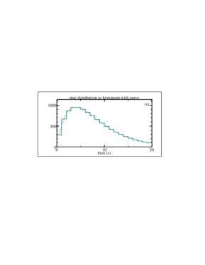
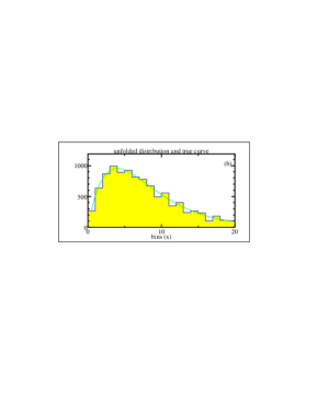
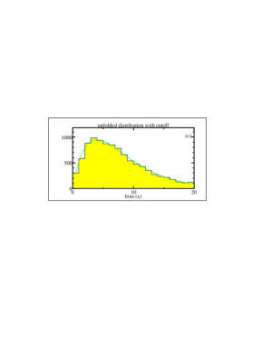
Figure 2: Original (true) distribution (a) and two results from unfolding ((b) and (c)). Result (b) has been obtained from all 20 coefficients, and for result (c) a sharp cut-off after 10 coefficients has been applied (i.e. the coefficients 11 to 20 are ignored).

Example. In a numerical example the matrix ${A}$ has the form of equation (8) with $n=20$ and a value of the migration parameter of $\varepsilon=0.22$. The first eigenvalue is $\lambda_{1}=1.0$, and the last one is $\lambda_{20}=1/7.9$, giving a condition number $\kappa=7.9$. For ${x}$ the ideal distribution of Figure 2a is assumed; the underlying function is of the form $x\exp(-ax)$. The decomposition of the matrix ${A}$ according to equation (9) is performed and the coefficients $b_{j}$ and $c_{j}$ are calculated. These coefficients are shown in Figure 3a (with $b_{j}\geq c_{j}$). In addition this figure shows, calculated by standard error propagation, the almost constant error level of the coefficients, of the folded distribution of Figure 2a with Poisson distributed bin contents. Figure 3a shows, that the coefficients $b_{j}$ of the true distribution decrease rapidly with increasing value $j$ of the index of the coefficient, by roughly three orders of magnitude. The coefficients $c_{j}$ of the folded distribution drop even faster, because it is more smooth due to the migration effect. Of course the relation $b_{j}/c_{j}=\lambda_{j}$ is valid. The last coefficient $b_{j}$ in Figure 3a is reduced to $c_{j}$ by the inverse of the condition number of the matrix, which is $\kappa=7.9$ in this case.

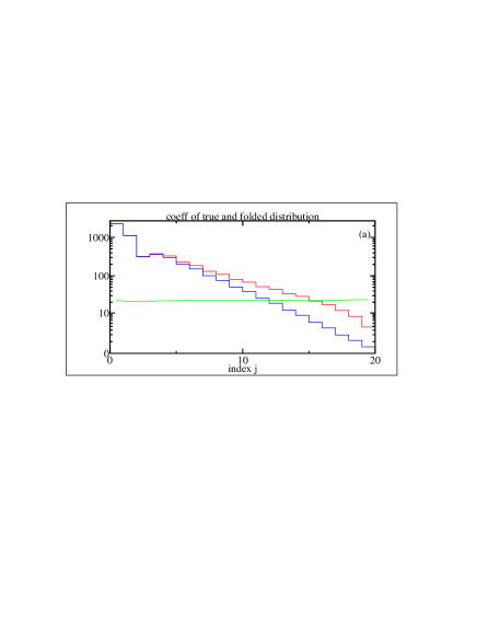
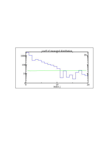
Figure 3: The absolute values of coefficients $b_{j}$ and $c_{j}$ are shown for $j=1,\,2,\ldots 20$. The coeffients $b_{j}$ and $c_{j}$ for the true distribution and the folded distribution (without measurement errors) are shown in (a), together with the (almost constant) error estimate for the coeffients $b_{j}$ calulated by error propagation. The coeffients $c_{j}$ from the simulated measured distribution are shown in (b), together with the error estimate. For $j$ above $12$ the smaller coefficients of the folded distribution become smaller than the statistical error. In (b) the coefficients for $j$ above $12$ are dominated by statistical errors and even the sign is not determined by the data.

The components of the first eigenvector $u_{1}$ (eigenvalue = 1) are all the same. Thus the coefficients $b_{i}$ and $c_{i}$ are identical, and proportional to the total sum of the measured distribution, not at all influenced by the migration. If visualized by functions, interpolating the components the eigenvector $u_{j}$ (eigenvalue $\lambda_{j}$) has $j-1$ zeros, and the curvature of the visualized eigenvectors is rapidly increasing with index $j$. The components of the last eigenvector $u_{n}$ have alternating sign for the bins; it has a small absolute value and its measured value will have a large relative statistical error. The value of $b_{20}$ is obtained by $b_{20}=7.9\cdot c_{20}$ in unfolding, introducing a large bin-to-bin oscillation into the result of unfolding.

In a simulation Poisson distributed bin contents are assumed in the measurement vector ${y}$. The coefficents for this measured distribution are shown in Figure 3b, together with the level of the statistical error. As expected from the size of the errors all coefficients with an index above about $j=12$ are dominated by the statistical error and therefore do not significantly contribute to the information content of the measurement. For indices above $j=12$ even the sign of the coeffient can not be determined by the measurement.

Using all the ”measured” coefficients for the unfolding the result of Figure 2b is obtained. This result shows large fluctuations around the expected values shown by the curve. The fluctuations are due to the contributions from indices above $j=12$, which represent noise and are magnified in the unfolding because of the large values of their inverse eigenvalues. The result is clearly unsatisfactory.

Because all measured coefficients $c_{j}$ with $j$ above a value of 12 are dominated by statistical errors (noise) their use in the unfolding makes no sense. A sharp cut-off after index $j=12$ or even after index $j=10$ will not remove any useful information from the measurement. The unfolding result using only measured coefficients $c_{j}$ up to $j=10$ is shown in Figure 2c; compared to Figure 2b the large fluctuations are suppressed and the results seems to be acceptable. Of course the fine structure of the true distribution expressed by the true coefficients $b_{j}$ with $j>10$ is not included in the solution and this may represent a bias. It is an unavoidable bias because these coefficients can not be measured.

The covariance matrix of the result can be calculated by standard error propagation. However it is clear that the covariance matrix is singular and has only rank 10 in this case, because the 20 bins are obtained from 10 measured coefficients (10 degrees of freedom). This property is inherent to the cut-off method and to the regularization method, and was already mentioned in [4]. Such singularity of the covariance matrix can be avoided if the final transformation is to a number of bins identical to the degree of freedoms; only a limited number of bins can be obtained in a measurement with large miration effects.

This method of using a sharp cut-off has to be compared to the regularization method. It has been shown [4] that the use of a regularization function of the type of equation (5) is equivalent to a smooth cut-off; essentially the measured coefficients $c_{j}$ are multiplied by a factor depending on the curvature of the orthogonal contributions (see section 3).

3 THE PROPOSED UNFOLDING METHOD

The proposed method is similar to the method used in RUN; the differences are emphasized in this section. It is expected that the proposed modifications results in more stable solutions. The proposed method requires large dimension parameters in the resolution matrix ${A}$. Like in RUN the regularization is determined by the required number of degrees of freedom, which determines the regularization parameter.

Figures in this section refer to the example already mentioned in section 1 In a Monte Carlo calculation of all three effects, limited ($x$-dependent) acceptance, non-linear transformation and finite resolution are simulated. Details on the function and the distorting effects are identical to the published examples [4]. In total 100 000 ”events” are simulated for ”data” and for the MC defining matrix ${A}$. The input function $f_{\text{MC}}(x)$ (equation (7)) is a constant.

In RUN the discretization for $f(x)$ and for $A(y,x)$ was done using cubic B-spline functions; the effect is the same as for simple histograms namely the integral equation is transformed to a system of linear equations, however the elements of the vectors are B-spline coefficients instead of bin contents. The advantage is that the parametrized solution is a smooth function and the curvature as defined by equation (5) can be exactly written as a quadratic form. However the accurate determination of matrix ${A}$ requires a good Monte Carlo statistic. In RUN statistical fluctuations of the elements of matrix ${A}$ could not be treated.

Simple histograms are instead proposed here; the elements of the vector ${y}$ are bin contents (integer numbers). The curvature of the solution is constructed by finite differences: the second derivative in bin $j$ is proportional to $x_{j-1}-2x_{j}+x_{j+1}$. In a histogram some resolution is lost if bins with a width as large as expected for the final resolution would be used. It is recommended to use initially $m=2n_{\text{df}}$ bins for ${x}$ for a final number of degrees of freedom of $n_{\text{df}}$. For $y$ a larger number of bins $n$ ($>m$) is recommended, to avoid a loss of resolution. Thus the number $n\times m$ of elements is large, and a large sample of Monte Carlo events is required to fill matrix ${A}$. The statistical error of the elements $a_{ij}$ eventually can not be neglected.

Standard Poisson maximum likelihood fit. Ignoring initially eventual statistical errors of the elements $a_{ij}$ the expected number of events in bin $i$ of ${y}$ is given by $y_{i}=\sum_{j=1}^{m}a_{ij}\,x_{j}$ . For the expected number $y_{i}$, as given by this expression, the observed values $\widehat{y}_{i}$ follows the Poisson distribution. Optimal estimates for the elements $x_{j}$ are obtained by minimizing the (negative) logarithm of the total likelihood with respect to the elements $x_{j}$ of vector ${x}$, assuming the Poisson distribution:

$$F(\mbox{\boldmath${x}$})=-\ln{\cal L}(\mbox{\boldmath${x}$})=-\ln\left[\prod_{i=1}^{n}P_{y_{i}}(\widehat{y}_{i})\right]=\sum_{i=1}^{n}\left(y_{i}-\widehat{y}_{i}\cdot\ln y_{i}\right)+\text{const.}\;,$$ (10)

where the constant term containing e.g $\widehat{y}_{i}!$ can be ommited. This expression (10) correctly accounts also for bins with a small number of histogram entries $\widehat{y}_{i}$.

An alternative would be to use the (linear) least squares method with singular value decomposition for the fit. However for small number of entries the use of the Poisson distribution seems to be essential. Furthermore the diagonalization used later in the method is almost equivalent to singular value decomposition (eigenvalues are the squares of the singular values).

Fitting with finite Monte Carlo samples. The problem of statistical fluctuations of the elements $a_{ij}$ has been neglected so far. A method to treat the problem within the maximum-likelihood method has been developed by R.Barlow and Chr.Beeston [9]. In this method there is for each source bin $x_{j}$ some (unknown) expected number of events $A_{ij}$. For each element $A_{ij}$ the corresponding number $a_{ij}$ from the Monte Carlo sample is generated by a distribution which is taken to be Poisson too. The nice feature of this method is that a bias which would be introduced by ignoring the statistical character of the values of the elements $a_{ij}$ is avoided and the maximum likelihood error is more realistic. A large number of slack variables (one for each bin) is introduced and has to be treated in the optimzation. A new fast numerical solution method has been developed (see [1]).

Combining bins. The likelihood function is a sum over all bins. Combining almost empty bins does not introduce a systematic error. The total number of elements of the matrix may be large, especially if $x$ and/or $y$ are multidimensional, and a small number of entries (or even zero) in an element may not be uncommon. The combination of almost empty bins is done with a cluster algorithm, taking into account the distance between bins in one, two or three dimensions.

First option: sharp cut-off of orthogonal contributions. This method is rather similar to the method discussed in section 2. The computational problem is to determine the minimum of $F(\mbox{\boldmath${x}$})$ (see equation (10)). The standard iterative method is based on the representation for the correction $\Delta\mbox{\boldmath${x}$}$

$$F(\Delta\mbox{\boldmath${x}$})=\frac{1}{2}\Delta\mbox{\boldmath${x}$}^{T}\mbox{\boldmath${H}$}\Delta\mbox{\boldmath${x}$}+\Delta\mbox{\boldmath${x}$}^{T}\mbox{\boldmath${g}$}+\ldots$$ (11)

with the Hessian ${H}$ (matrix of second derivatives of $F(\Delta\mbox{\boldmath${x}$})$) and the gradient vector ${g}$ (first derivatives of $F(\Delta\mbox{\boldmath${x}$})$). A Newton step is then calulated from equation $\mbox{\boldmath${H}$}\Delta\mbox{\boldmath${x}$}+\mbox{\boldmath${g}$}=0$. Convergence is usually fast for good starting values and the covariance matrix is equal to the inverse of the Hessian. The starting values can be calculated by a linear least square fit, based on the approximation of the Poisson distribution by a Gaussian distribution for each bin.

A sharp cut-off as discussed in the example of section 2 requires a diagonalization of the symmetric matrix ${H}$ by $\mbox{\boldmath${H}$}=\mbox{\boldmath${U}$}\mbox{\boldmath${D}$}\,\mbox{\boldmath${U}$}^{T}$ with a diagonal matrix ${D}$ and a transformation matrix ${U}$. By a transformation (rotation) in ${x}$-space linear combinations of the ${x}$-components are obtained with a diagonal covariance matrix, with variances of the linear combinations given by the inverse of the eigenvalues of matrix ${D}$. A cut-off is done at some index $j$ followed by backtransformation to the ${x}$-space of bin-contents using the transformation matrix ${U}$.

Second option: regularization. In this option the regularization is based on the second derivative of the result according to equation (5), which can be expressed by a quadratic form $\mbox{\boldmath${x}$}^{T}\mbox{\boldmath${C}$}\mbox{\boldmath${x}$}$ with a positive-semidefinite matrix ${C}$. In principle the same procedure is used as in RUN; the mathematical details are given elsewhere [4]. Here a simple explanation is given on the standard mathematical operations used. Regularization is done by adding the term $\tau\cdot\mbox{\boldmath${x}$}^{T}\mbox{\boldmath${C}$}\mbox{\boldmath${x}$}$ to the function $F(\Delta\mbox{\boldmath${x}$})$ of equation (11). Exactly as in the first option the Hessian is diagonalized.

$$\mbox{\boldmath${H}$}=\mbox{\boldmath${U}$}\mbox{\boldmath${D}$}\,\mbox{\boldmath${U}$}^{T}\qquad\qquad\qquad\mbox{\boldmath${H}$}^{-1}=\mbox{\boldmath${U}$}\mbox{\boldmath${D}$}^{-1}\mbox{\boldmath${U}$}^{T}=\left[\mbox{\boldmath${U}$}\mbox{\boldmath${D}$}^{-1/2}\right]\left[\mbox{\boldmath${D}$}^{-1/2}\mbox{\boldmath${U}$}^{T}\right]\;.$$ (12)

Up to this step everything is identical to the cut-off option. Using transformation matrix $\mbox{\boldmath${U}$}\mbox{\boldmath${D}$}^{-1/2}$ the vector ${x}$ is transformed to linear combinations $\widehat{\mbox{\boldmath${x}$}}$, which are orthogonal, with all variances equal to 1 (unit covariance matrix). Because the covariance matrix is equal to the unit matrix, every additional pure rotation will not change the (unit) covariance matrix. In terms of the transformed vector the regularization term can now be written in the form $\tau\cdot\widehat{\mbox{\boldmath${x}$}}^{T}C_{U}\widehat{\mbox{\boldmath${x}$}}$, where $C_{U}$ is the transformed curvature matrix ${C}$. Now another diagonalization can be done of matrix $C_{U}$:

$$\tau\cdot\mbox{\boldmath${x}$}^{T}\mbox{\boldmath${C}$}\mbox{\boldmath${x}$}\;\to\;\tau\cdot\widehat{\mbox{\boldmath${x}$}}^{T}\mbox{\boldmath${C}$}_{U}\widehat{\mbox{\boldmath${x}$}}=\tau\cdot\widehat{\mbox{\boldmath${x}$}}^{T}\mbox{\boldmath${U}$}_{C}\;\mbox{\boldmath${S}$}\;\mbox{\boldmath${U}$}_{C}^{T}\widehat{\mbox{\boldmath${x}$}}$$ (13)

with a diagonal matrix ${S}$ and a rotation matrix $\mbox{\boldmath${U}$}_{C}$. This diagonalization can be used to define a pure rotation from the linear combination $\widehat{\mbox{\boldmath${x}$}}$ to another linear combination $\widetilde{\mbox{\boldmath${x}$}}$

$$\widehat{\mbox{\boldmath${x}$}}\;\to\;\widetilde{\mbox{\boldmath${x}$}}=\mbox{\boldmath${U}$}_{C}^{T}\,\widehat{\mbox{\boldmath${x}$}}\;.$$ (14)

The components of the new vector $\widetilde{\mbox{\boldmath${x}$}}$ still have the unit matrix as covariance matrix. The complete transformation from ${x}$ to $\widetilde{\mbox{\boldmath${x}$}}$ is the effect of the transformation by $\mbox{\boldmath${U}$}\mbox{\boldmath${D}$}^{-1/2}$ and by $\mbox{\boldmath${U}$}_{C}$. The algebra can be explained in other words: the error ellipsoid related to the Hessian is first rotated to have the axes parallel to the axes of the new system. By a change of the scales the ellipsoid is transformed to a sphere, which will remain a sphere for any further rotation. A last rotation is done to bring the axes into the order of increasing curvature.

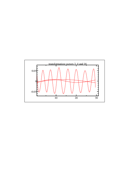
Figure 4: Selected column vectors of the complete transformation matrix defined in the regularization procedure. They correspond to the curvature eigenvalues $S_{33}$, $S_{44}$ and $S_{16,16}$. Visualization is done by curves interpolating the components. The amplitude associated which each vector all have the same standard deviation of 1.

Some columns of the complete (product) transformation are shown in Figure 4. All linear combinations obtained have the same precision (standard deviation of the coefficient is one). As seen in the Figure linear combinations with large index $j$ are oscillating with large amplitude. The diagonal elements $S_{jj}$ are the (statistically independent) contributions of the elements of $\widetilde{\mbox{\boldmath${x}$}}$ to the total curvature. Sorted according to increasing value of $S_{jj}$ the value of $S_{jj}$ will increase rather fast with increasing index $j$. The spectrum of eigenvalues $S_{jj}$ is shown in Figure 5. In terms of the linear combinations $\widetilde{\mbox{\boldmath${x}$}}$ regularization is simply given by

$$\left(\widetilde{x}_{j}\right)_{\text{reg}}=\left(\frac{1}{1+\tau\cdot S_{jj}}\right)\left(\widetilde{x}_{j}\right)_{\text{unreg}}\;.$$ (15)

and this simple form is the reason for the transformations made before.

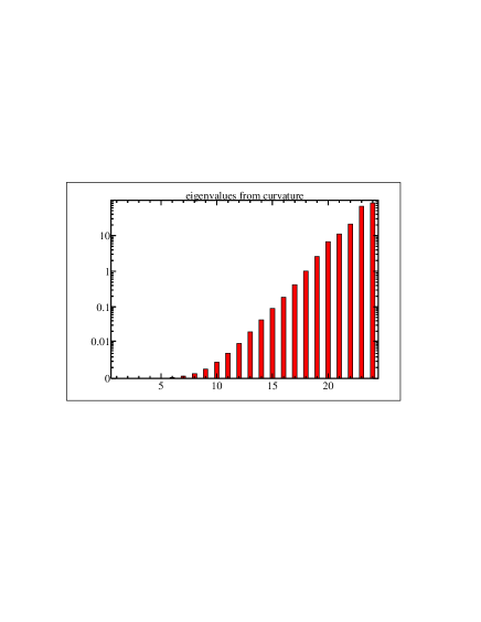
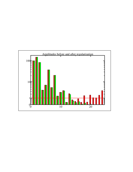
Figure 5: The eigenvalues after the curvature transformation. The values are very rapidly increasing for orthogonal contributions for increasing index value (left). The amplitudes before (left bars) and after regularization (right bars). The statistical error of all amplitudes is equal to 1, which is indicated by the horizontal line. The vertical scale is linear at the bottom and makes a transition to a logarithmic scale at the top (right).

Determination of the regularization parameters $\tau$. The first factors (small $j$) on the right-hand-side of equation (15) will be close to 1; for a value $\tau=1/S_{kk}$ the factor will be 1/2 and for indices $j>k$ will rapidly decrease towards zero. The sum of all factors can be called the effective number of degrees of freedom, and can be used to determine the value of the regularization parameter $\tau$ from the required number of degrees of freedom, i.e. the regularization parameter $\tau$ is determined from the value of $n_{\text{df}}$ in the equation

$$n_{\text{df}}=\sum_{j=1}^{m}\left(\frac{1}{1+\tau\cdot S_{jj}}\right)\;.$$ (16)

Thus the required number of degrees of freedom has to be specified and determines the degree of regularization. This number can be taken from the spectrum of the coefficients or amplitudes, shown in Figure 5. The insignificant part (large $j$) is clearly visible in the spectrum and separated from the significant part (small $j$). The selected value of $n_{df}$ should be equal to or larger than the number of significant terms. The unregularized amplitudes, which have standard deviation one, are shown by the left bars; amplitudes above index 15 are compatible with one and represent noise. They would however make a large contribution to the solution, because the corresponding column vectors (Figure 4) are large. The regularization effectively damps the amplitude (right bars) around and above index 15, which has been chosen as the degree of freedom here. The significant amplitudes are not affected by the regularization.

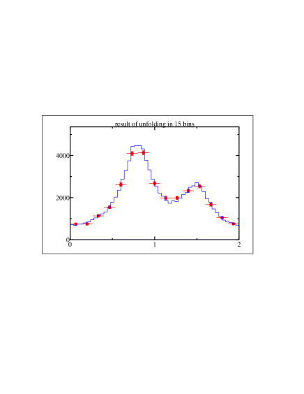
Figure 6: The unfolding result after regularization with 15 degrees of freedom with 30 bins (left) and with 15 bins (right). For comparison the original (true) distribution is shown by a histogram. The data from Figure 1 are used as input.

The final result of the example (measured distribution in Figure 1) is shown in Figure 6. The left figure shows 30 data points with error bars together with the original (true) distribution; within errors the original distribution is nicely reproduced. The rank of the covariance matrix is about 15, which was chosen as the effective number of degrees of freedom; thus inversion of the covariance matrix, needed e.g. for a least-square fit of a model to the data, is not possible. Although the large number of 30 data points seems to be attractive, the data points should be reduced to 15 data points by combining two bins to one, which then have a full-rank covariance matrix. This set of data points is shown in Figure 6 (right). The broader bins of this set of data points are a consequence of the limited acceptance and finite resolution of the measurement.

References

-
[1]
A more detailed text is available
via
http://www.desy.de/~blobel/. - [2] D. L. Phillips , A technique for the numerical solution of certain integral equations of the first kind, J. Assoc. Comput. Mach. 9, 84-97 (1962)
- [3] A.N. Thikhonov, On the solution of improperly posed problems and the method of regularization, Sov. Math. 5, 1035 (1963)
- [4] V. Blobel, Unfolding methods in high energy physics experiments, in Proceedings of the 1984 CERN School of Computing, CERN 85-09 (1985) and DESY 84-114
- [5] V. Blobel, The manual, Regularized Unfolding for High-Energy Physics Experiments, OPAL Technical Note TN361 (1996)
- [6] M. Jonker et al. (CHARM Collaboration), Experimental study of differential cross sections in neutral current neutrino and antineutrino interactions Physics Letters 102 B, 62-72 (1981) M. Jonker et al. (CHARM Collaboration), Experimental study of -distributions in semileptonic neutral current neutrino interactions, Physics Letters 128 B, 117-123 (1983)
- [7] Ch. Berger et al. (PLUTO Collaboration), Measurement of the photon structure function , Physics Letters 142 B, 111-118 (1984) Ch. Berger et al. (PLUTO Collaboration), Measurement of deep inelastic electron scattering off virtual photons, Physics Letters 142 B, 119-124 (1984)
- [8] A.K. Louis, Inverse und schlecht gestellte Probleme, Teubner, Stuttgart und Leipzig (1989)
- [9] Roger Barlow and Christine Beeston, Fitting finite Monte Carlo samples, Computer Physics Communications 77, 219–228 (1993)