A Dalitz plot analysis of the $D^{0}$ hadronic decays $D^{0}\rightarrow K^{0}K^{-}\pi^{+}$, $D^{0}\rightarrow\overline{K}^{0}K^{+}\pi^{-}$ and $D^{0}\rightarrow\overline{K}^{0}K^{+}K^{-}$ is presented. This analysis is based on a data sample of 22 $\mbox{\,fb}^{-1}$ collected with the BABAR detector at the PEP-II asymmetric-energy B Factory at SLAC running on or near the $\mathchar 28935\relax{(4S)}$ resonance. The events are selected from continuum $e^{+}e^{-}$ annihilations using the decay $D^{*+}\rightarrow D^{0}\pi^{+}$. Preliminary measurements of the branching fractions of the above hadronic decays are obtained. Preliminary estimates of fractions and phases for resonant and nonresonant contributions to the Dalitz plot are also presented.

Contributed to the 31^st International Conference on High Energy Physics,

7/24—7/31/2002, Amsterdam, The Netherlands

1 Introduction

The Dalitz plot analysis is the most complete method of studying the dynamics of three-body charm decays. These decays are expected to proceed through intermediate resonant two-body modes [1] and experimentally this is the observed pattern with some important exceptions. In the case of the decay $D^{+}\rightarrow K^{-}\pi^{+}\pi^{+}$ [2], for example, the data can be described with a large ($\approx$ 90%) nonresonant contribution. Dalitz plot analyses can provide new information on the resonances that contribute to observed three-body final states.

In addition, since the intermediate two-body modes are dominated by light mesons, new information on light meson spectroscopy can be obtained. In particular, old puzzles related to the parameters and the internal structure of several light mesons can receive new inputs.

This paper focuses on the study of three-body $D^{0}$ meson decays involving a $K^{0}$ (where $K^{0}\rightarrow\pi^{+}\pi^{-}$) such as

$$D^{0} \rightarrow\overline{K}^{0}\pi^{+}\pi^{-},$$ (1)

$$D^{0} \rightarrow K^{0}K^{-}\pi^{+},$$ (2)

$$D^{0} \rightarrow\overline{K}^{0}K^{+}\pi^{-},$$ (3)

$$D^{0} \rightarrow\overline{K}^{0}K^{+}K^{-}.$$ (4)

When decays (2) and (3) are combined, they are labelled as $D^{0}\rightarrow K^{0}K\pi$. All decays are collectively referred to as $K^{0}h^{+}h^{-}$.

2 The BABAR Detector and Dataset

The data sample used in this analysis consists of 22 $\mbox{\,fb}^{-1}$ recorded with the BABAR detector at the SLAC PEP-II storage ring between October 1999 and December 2000. The PEP-II facility operates nominally at the $\mathchar 28935\relax{(4S)}$ resonance, providing collisions of 9.0 $\mathrm{\,Ge\kern-1.00006ptV}$ electrons on 3.1 $\mathrm{\,Ge\kern-1.00006ptV}$ positrons. The data set includes 19.6 $\mbox{\,fb}^{-1}$ collected in this configuration (on-resonance) and 2.4 $\mbox{\,fb}^{-1}$ collected below the $B\kern 1.79993pt\overline{\kern-1.79993ptB}{}$ threshold (off-resonance).

A more complete overview of the BABAR detector can be found elsewhere [3]. The following is a brief description of the components important for this analysis. The interaction point is surrounded by a 5-layer double-sided silicon vertex tracker (SVT) and a 40-layer drift chamber (DCH) filled with a gas mixture of helium and isobutane in a 1.5 T superconducting solenoidal magnet. In addition to providing precise spatial hits for tracking, the SVT and DCH also measure $dE/dx$, which provides particle identification for low-momentum charged particles. At higher momenta ($p>0.7$ ${\mathrm{\,Ge\kern-1.00006ptV\!/}c}$) pions and kaons are identified by Cherenkov radiation observed in the DIRC, a detector designed to measure internally reflected Cherenkov light. The typical separation between pions and kaons varies from $8\sigma$ at 2 ${\mathrm{\,Ge\kern-1.00006ptV\!/}c}$ to 2.5$\sigma$ at 4 ${\mathrm{\,Ge\kern-1.00006ptV\!/}c}$, where $\sigma$ is the experimental resolution for the measurement of the Cherenkov angle.

3 Event Selection and $D^{0}$ Reconstruction

The decay $D^{*+}\rightarrow D^{0}\pi^{+}$ is used to distinguish between $D^{0}$ and $\overline{D^{0}}$ and to reduce background. For example, the Cabibbo-favored decays are

$$D^{*+}\rightarrow\begin{array}[t]{l}D^{0}\pi^{+}\\ \rightarrow\overline{K}^{0}\pi^{+}\pi^{-},\end{array}$$

$$D^{*-}\rightarrow\begin{array}[t]{l}\overline{D^{0}}\pi^{-}\\ \rightarrow K^{0}\pi^{+}\pi^{-}.\end{array}$$

The charge of the slow $\pi^{\pm}$ from $D^{*}$ decay (referred to as the slow pion) identifies the flavor of the $D^{0}$ and $K^{0}$ (apart from a small contribution from doubly-Cabibbo-suppressed decays). The decay channels $K^{0}K^{-}\pi^{+}$ and $\overline{K}^{0}K^{+}\pi^{-}$ are produced by different decay diagrams, as shown in Fig. 1; therefore their rates are not expected to be the same.

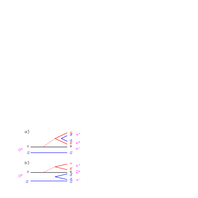
Figure 1: Diagrams that contribute to (a) $D^{0}\rightarrow K^{0}K^{-}\pi^{+}$ and (b) $D^{0}\rightarrow\overline{K}^{0}K^{+}\pi^{-}$.

$D^{0}\rightarrow K^{0}h^{+}h^{-}$ candidates are reconstructed from $K^{0}_{S}\rightarrow\pi^{+}\pi^{-}$ candidates plus two charged tracks, each with at least 12 hits in the DCH, and a track with momentum smaller than 0.6 ${\mathrm{\,Ge\kern-1.00006ptV\!/}c}$ with at least 6 hits in the SVT. In addition, tracks are required to have transverse momentum $p_{T}>$ 100 MeV/$c$ and, except for the $K^{0}$ decay pions, to point back to the nominal interaction point within 1.5 cm transverse to the beam and 3 cm along the beam direction.

$K^{0}$ particles are reconstructed by kinematically fitting all pairs of positive and negative tracks. Reconstructed $K^{0}$ candidates are then fit to a common vertex with all remaining combinations of pairs of positive and negative tracks. Fake $K^{0}$ candidates are removed requiring a flight distance of 0.4 cm with respect to the candidate $D^{0}$ vertex. The $D^{0}$ candidate is then combined with all the slow pion candidates, which are refitted to a common vertex constrained to be located in the interaction region. In all cases a fit probability cut at 0.1 % is applied.

In order to reduce the combinatorial background, $D^{0}$ particles originating from $B$ decays are rejected by requiring that the center of mass momentum of the $D^{0}$ candidate is greater than 2.2 ${\mathrm{\,Ge\kern-1.00006ptV\!/}c}$.

Two different particle identification algorithms (PID) are used for kaon identification, both of which take advantage of the measurement of $dE/dx$ in the tracking detectors and a measurement of the Cherenkov angle in the DIRC. The first employs less stringent requirements and has an efficiency above 95% for kaons with momentum less than 3 ${\mathrm{\,Ge\kern-1.00006ptV\!/}c}$ and $\pi$ misidentification probability of about 20%. The second algorithm is more strict and has kaon identification efficiencies of 70% to 90% in the same momentum range but with $\pi$ misidentification probabilities below 7%. The more permissive $K$ identification algorithm is used for the measurement of branching ratios, where more uniform acceptance is desirable, and the tighter $K$ algorithm is used for the Dalitz plot analyses, where background reduction is more important.

Each $D^{0}$ sample is characterized by the distributions of two variables, the invariant mass of the candidate $D^{0}$, and the difference between the invariant masses of the $D^{*}$ and $D^{0}$ candidates,

$$\Delta m=m(K^{0}h^{+}h^{-}\pi_{S}^{+})-m(K^{0}h^{+}h^{-}),$$

where $\pi^{+}_{S}$ is the slow pion. The distribution of $\Delta m$ for those candidates that fall within 2.5 $\sigma$ of the $D^{0}$ mass peak is shown in Fig. 2. A strong $D^{*}$ signal is apparent. Fits to these distributions produce consistent means and widths for the four channels ($\sigma=(323\pm 10)$ ${\mathrm{\,ke\kern-1.00006ptV\!/}c^{2}}$ in the case of decay channel $\overline{K}^{0}\pi^{+}\pi^{-}$). The $K^{0}h^{+}h^{-}$ mass distribution for candidates that fall within $\pm 969$ ${\mathrm{\,ke\kern-1.00006ptV\!/}c^{2}}$ (corresponding to 3 $\sigma$) from the central value of the $\Delta m$ distribution is shown in Fig. 3.

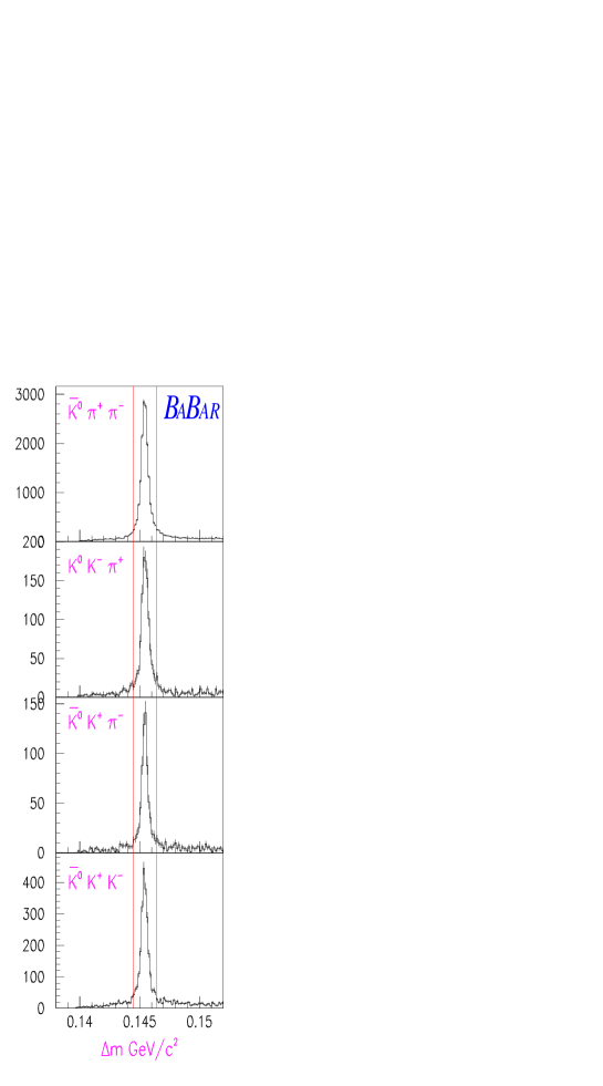
Figure 2: $\Delta m$ distributions for $D^{0}\rightarrow K^{0}h^{+}h^{-}$ candidates, for events in which the $K^{0}h^{+}h^{-}$ invariant mass is within 2.5 $\sigma$ of the $D^{0}$ mass. The lines represent the range of $\Delta m$ used to select the $D^{0}$ candidates.

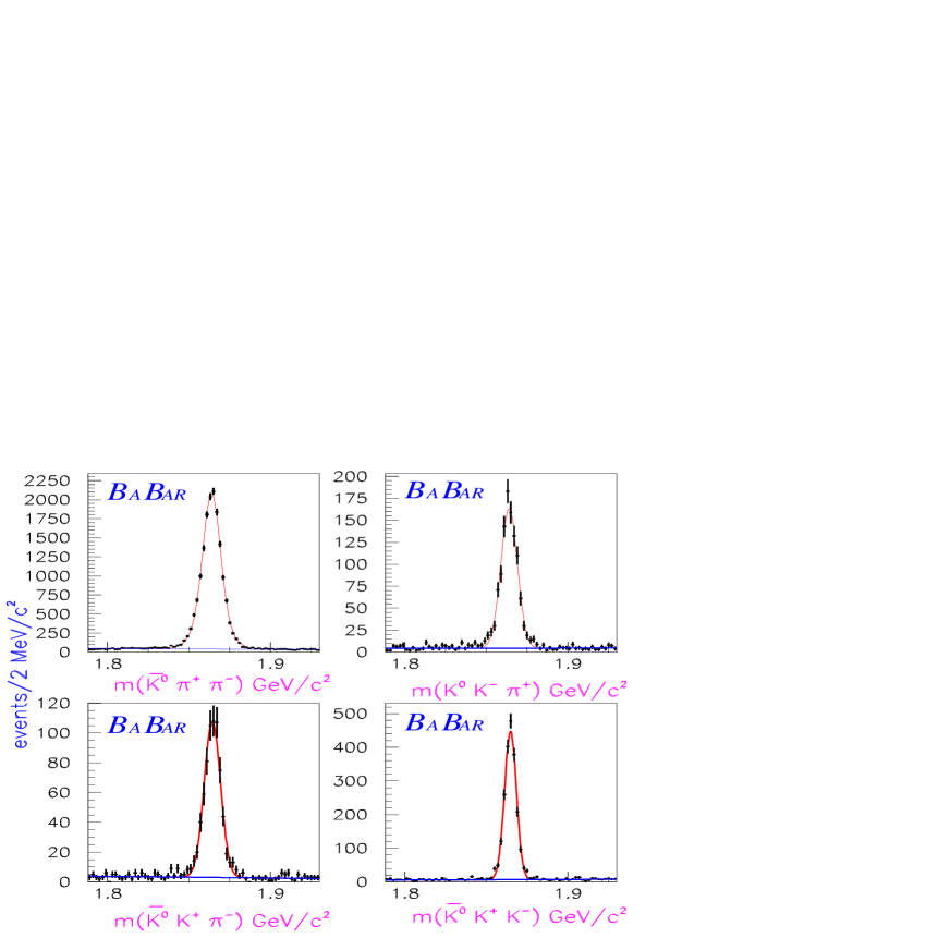
Figure 3: $K^{0}h^{+}h^{-}$ mass distributions for events in which $\Delta m$ is within 969 ${\mathrm{\,ke\kern-1.00006ptV\!/}c^{2}}$ of the mean $\Delta m$ value for signal events.

4 Efficiency

The efficiency for the decays in the four $D^{0}$ samples is determined from a sample of Monte Carlo events in which each decay mode is generated according to uniform phase space (such that the Dalitz plot is uniformly populated). These events are passed through a full detector simulation based on GEANT3 [4] and subjected to the same reconstruction and event selection as the data. The distribution of these events in the Dalitz plot after selection is used to determine the reconstruction efficiency. Typical Monte Carlo samples used to compute these efficiencies consist of 400 $\times 10^{3}$ events.

This Dalitz distribution is divided into small cells and fit to a third-order polynomial in two dimensions. Cells with less than 50 events are ignored in the fit. The resulting $\chi^{2}$ per number of degrees of freedom ($\chi^{2}/NDF$) is typically 1.1. The fitted efficiencies are shown in Fig. 4. The average over the Dalitz plot ranges from 7.3% to 8.7%, depending on the decay mode.

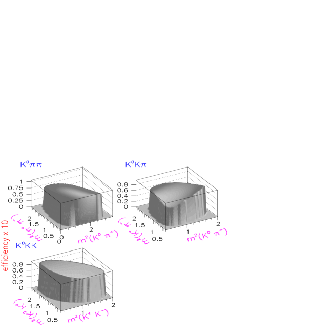
Figure 4: Dalitz plot efficiency ($\times$ 10) for $D^{0}\rightarrow\overline{K}^{0}\pi^{+}\pi^{-}$, $D^{0}\rightarrow K^{0}K\pi$ and $D^{0}\rightarrow\overline{K}^{0}K^{+}K^{-}$.

5 Branching Fractions

Since all four decay channels $K^{0}h^{+}h^{-}$ have similiar topologies, the ratios of branching fractions, calculated relative to the $\overline{K}^{0}\pi^{+}\pi^{-}$ decay mode, are expected to have relatively small systematic uncertainties. These ratios are evaluated as

$$R=\frac{\sum_{x,y}\frac{N_{i}(x,y)}{\epsilon_{i}(x,y)}}{\sum_{x,y}\frac{N_{1}(x,y)}{\epsilon_{1}(x,y)}},$$

where $N_{i}(x,y)$ represents the number of events measured for channel $i$ and $\epsilon_{i}(x,y)$ is the corresponding efficiency in a given Dalitz plot cell $(x,y)$ .

In order to obtain the yields and measure the relative branching fractions, the $K^{0}h^{+}h^{-}$ mass distributions are fit with a Gaussian function and a linear background. The number of signal events is calculated as the difference between the total number of events within $3\sigma$ of the $D^{0}$ mass from the fit and the integrated linear background function in the same mass range. The results obtained with this procedure are summarized in Table 1.

Table 1: Results from the fits to the $K^{0}h^{+}h^{-}$ mass distributions. The fits are performed using a linear background and a Gaussian function for the signal.

Channel	mass (MeV/$c^{2}$)	$\sigma$ (MeV/$c^{2}$)	signal events
$D^{0}\rightarrow\overline{K}^{0}\pi^{+}\pi^{-}$	1863.9 $\pm$ 0.5	6.29 $\pm$ 0.05	15 279 $\pm$ 129
$D^{0}\rightarrow K^{0}K^{-}\pi^{+}$	1863.9 $\pm$ 0.2	5.1 $\pm$ 0.2	1 165 $\pm$ 40
$D^{0}\rightarrow\overline{K}^{0}K^{+}\pi^{-}$	1864.3 $\pm$ 0.2	5.0 $\pm$ 0.2	805 $\pm$ 35
$D^{0}\rightarrow\overline{K}^{0}K^{+}K^{-}$	1864.7 $\pm$ 0.8	3.6 $\pm$ 0.1	2 109 $\pm$ 48

Systematic errors take into account the different algorithms used for particle identification and the way in which the Dalitz plot efficiency is used to correct the data. For example, the full data set is divided into two samples corresponding to different DCH high voltage operating points and the branching ratios are computed separately for the two samples. Differences in the branching ratios are used as an estimate of systematic uncertainties. The contributions to the systematic errors are summarized in Table 2. The total error is obtained by adding in quadrature the single contributions.

Table 2: Contributions to the systematic error on the ratio of branching fractions relative to $D^{0}\rightarrow\overline{K}^{0}\pi^{+}\pi^{-}$ (%) from different sources.

Channel	PID	Efficiency correction	DCH voltage	Total
$D^{0}\rightarrow K^{0}K^{-}\pi^{+}$	0.31	0.14	0.45	0.56
$D^{0}\rightarrow\overline{K}^{0}K^{+}\pi^{-}$	0.18	0.04	0.37	0.41
$D^{0}\rightarrow\overline{K}^{0}K^{+}K^{-}$	0.19	0.09	0.17	0.27

The method for measuring the branching ratios is checked with a different fully inclusive $e^{+}e^{-}\rightarrow\bar{c}c$ Monte Carlo sample in which the $D^{0}$ mesons decay according to the PDG [5] branching fractions. The Monte Carlo events are subjected to the same reconstruction, event selection and analysis as the real data. The size of this Monte Carlo sample is comparable to that of the data sample. The results are found to be statistically consistent with the branching ratios assumed in the Monte Carlo generation.

The measured preliminary ratios of branching fractions are shown in Table 3 and are compared with those measured by other experiments.

Table 3: Ratio of branching fractions relative to $D^{0}\rightarrow\overline{K}^{0}\pi^{+}\pi^{-}$ (%). Note that ARGUS did not separate $K^{0}K^{-}\pi^{+}$ from $\overline{K}^{0}K^{+}\pi^{-}$.

Channel	BABAR	CLEO [6]	ARGUS [7]	E691 [8]
$D^{0}\rightarrow K^{0}K^{-}\pi^{+}$	8.32 $\pm$ 0.29 (stat) $\pm$ 0.56(syst)	10.8 $\pm$ 1.9	16.0 $\pm$ 3.0	12.4 $\pm$ 4.7
$D^{0}\rightarrow\overline{K}^{0}K^{+}\pi^{-}$	5.68 $\pm$ 0.25(stat) $\pm$ 0.41(syst)	9.8 $\pm$ 2.0		7.8 $\pm$ 3.9
$D^{0}\rightarrow\overline{K}^{0}K^{+}K^{-}$	16.30 $\pm$ 0.37(stat) $\pm$ 0.27(syst)	17.0 $\pm$ 2.2

6 Dalitz Plot Analysis Method

An unbinned maximum likelihood fit is performed for the decay modes $D^{0}\rightarrow K^{0}K^{-}\pi^{+}$, $D^{0}\rightarrow\overline{K}^{0}K^{+}\pi^{-}$ and $D^{0}\rightarrow\overline{K}^{0}K^{+}K^{-}$, in order to use the distribution of events in the Dalitz plot to determine the relative amplitudes and phases of intermediate resonant and nonresonant states.

Following the method used by ARGUS [9] and CLEO [10], the likelihood function is written in the following way:

$$L=\beta\cdot G(m)\frac{\sum_{i,j}c_{i}c_{j}^{*}A_{i}A_{j}^{*}}{\int{\sum_{i,j}c_{i}c_{j}^{*}A_{i}A_{j}^{*}\epsilon(m_{x}^{2},m_{y}^{2})}dm_{x}^{2}dm_{y}^{2}}+\frac{(1-\beta)}{\int\epsilon(m_{x}^{2},m_{y}^{2})dm_{x}^{2}dm_{y}^{2}}.$$ (5)

In this expression, $\beta$ represents the fraction of signal obtained from the fit to the mass spectrum and $\epsilon(m_{x}^{2},m_{y}^{2})$ is the Dalitz plot efficiency. $G(m)$ is a Gaussian function describing the $D^{0}$ lineshape normalized within the $2\sigma$ cut used to perform the Dalitz plot analysis. It is assumed that the background events, described by the second term in Eq. 5, uniformly populate the Dalitz plot. This assumption is verified by examining events in the $D^{0}$ side bands. The output from the fit is the set of complex coefficients $c_{i}$.

In Eq. 5, the integrals are computed using Monte Carlo events taking into account the Dalitz plot efficiency. The branching fraction for the resonant or nonresonant contribution $i$ is defined by the following expression:

$$f_{i}=\frac{|c_{i}|^{2}\int|A_{i}|^{2}dm_{x}^{2}dm_{y}^{2}}{\sum_{j,k}c_{j}c_{k}^{*}\int A_{j}A_{k}^{*}dm_{x}^{2}dm_{y}^{2}}.$$

The fractions $f_{i}$ do not necessarily add up to 1 because of interference between amplitudes. The errors in the fractions are evaluated by propagating the full covariance matrix obtained by the fit.

The phase of each amplitude is measured with respect to the mode with the largest amplitude. The amplitudes $A_{i}$ are each represented by the product of a complex Breit-Wigner function and an angular function (the Zemach tensors [11]):

$$A=BW(m)\times T(\mathchar 28938\relax).$$

The Breit-Wigner function includes Blatt-Weisskopf form factors [12]. The $f_{0}(980)$ and $a_{0}(980)$ resonances is described using coupled-channel Breit-Wigner functions with parameters taken from the CERN/WA76 [13] and the Crystal Barrel [14] experiments, respectively. The parameters of the $\phi(1020)$ meson are extracted from the data ($\Gamma=(4.3\pm 0.3)$ MeV/$c^{2}$) since the apparent width is affected by the experimental resolution. The resonance parameters of the $K^{*}_{0}(1430)$ are $m=1.435$ ${\mathrm{\,Ge\kern-1.00006ptV\!/}c^{2}}$ and $\Gamma$=279 ${\mathrm{\,Ge\kern-1.00006ptV\!/}c^{2}}$ from a recent reanalysis of elastic $K\pi$ scattering data from the LASS experiment [15]. The nonresonant contribution (N.R.) is represented by a constant term with a free phase.

The fit quality is evaluated in the following way. The Dalitz plot is re-binned into $N_{cells}$ cells grouping together bins with small event yields. Then a Monte Carlo sample is generated with parameters from the fit to data. This distribution is used to evaluate a $\chi^{2}$ for the Dalitz plot. The $\chi^{2}/N_{cells}$ is displayed in Table 4 for the fit results shown in Tables 5, 6, and 7, together with the event yield and purity for each of the three channels used in the Dalitz plot analyses.

Table 4: Event yields, purity and $\chi^{2}/N_{cells}$ for the three channels in the Dalitz plot analyses.

$D^{0}$ Decay mode	Events	Purity (%)	$\chi^{2}/N_{cells}$
$D^{0}\rightarrow K^{0}K^{-}\pi^{+}$	1008	95.5 $\pm$ 0.4	46/44
$D^{0}\rightarrow\overline{K}^{0}K^{+}\pi^{-}$	659	95.5 $\pm$ 0.4	25/29
$D^{0}\rightarrow\overline{K}^{0}K^{+}K^{-}$	1957	97.5 $\pm$ 0.2	98/59

Systematic errors on the fitted fractions are evaluated by making different assumptions in the fits — for example, we have performed fits with the Blatt-Weisskopf terms set to 1, and with uniform efficiency across the Dalitz plot.

7 $D^{0}\rightarrow K^{0}K^{-}\pi^{+}$ Dalitz Plot Analysis

The Dalitz plot for $D^{0}\rightarrow K^{0}K^{-}\pi^{+}$ candidates is shown in Fig. 5 and its projections are shown in Fig. 6. The presence of a strong $K^{*+}(892)$ resonance can be observed. Table 5 shows the list of intermediate final states and the fitted fractions for this decay channel.

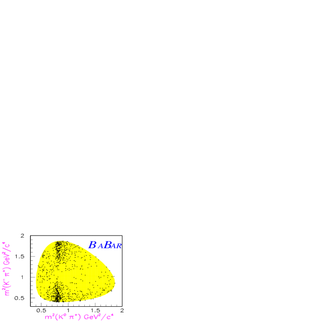
Figure 5: Dalitz plot of $D^{0}\rightarrow K^{0}K^{-}\pi^{+}$.

Table 5: Preliminary results from the Dalitz plot analysis of $D^{0}\rightarrow K^{0}K^{-}\pi^{+}$.

Final state	Fraction (%)	Phase (degrees)
$\kern 1.99997pt\overline{\kern-1.99997ptK}{}^{*0}_{0}(1430)K^{0}$	4.8 $\pm$ 1.4 $\pm$ 1.6	52 $\pm$ 27
$\kern 1.99997pt\overline{\kern-1.99997ptK}{}^{*0}_{1}(892)K^{0}$	0.8 $\pm$ 0.5 $\pm$ 0.1	175 $\pm$ 22
$\kern 1.99997pt\overline{\kern-1.99997ptK}{}^{*0}_{1}(1680)K^{0}$	6.9 $\pm$ 1.2 $\pm$ 1.0	–169 $\pm$ 16
$\kern 1.99997pt\overline{\kern-1.99997ptK}{}^{*0}_{2}(1430)K^{0}$	2.0 $\pm$ 0.6 $\pm$ 0.1	51 $\pm$ 18
$K^{*+}_{0}(1430)K^{-}$	13.3 $\pm$ 3.5 $\pm$ 3.9	–41 $\pm$ 25
$K^{*+}_{1}(892)K^{-}$	63.6 $\pm$ 5.1 $\pm$ 2.6	0
$K^{*+}_{1}(1680)K^{-}$	15.6 $\pm$ 3.0 $\pm$ 1.4	–178 $\pm$ 10
$K^{*+}_{2}(1430)K^{-}$	13.8 $\pm$ 2.6 $\pm$ 7.9	–52 $\pm$ 7
$a_{0}^{-}(980)\pi^{+}$	2.9 $\pm$ 2.3 $\pm$ 0.7	–100 $\pm$ 13
$a_{0}^{-}(1450)\pi^{+}$	3.1 $\pm$ 1.9 $\pm$ 0.9	31 $\pm$ 16
$a_{2}^{-}(1310)\pi^{+}$	0.7 $\pm$ 0.4 $\pm$ 0.1	–149 $\pm$ 27
N.R.	2.3 $\pm$ 0.5 $\pm$ 5.6	–136 $\pm$ 23
Sum	130 $\pm$ 8

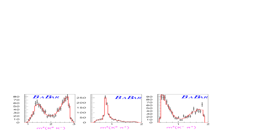
Figure 6: Dalitz plot projections for $D^{0}\rightarrow K^{0}K^{-}\pi^{+}$. The data are represented with error bars; the histogram is a projection of the fit described in the text.

The results from the fit, shown in Table 5, confirm that the channel is dominated by $K^{*}$ resonances in the charged mode. Contributions from neutral $K^{*}$ as well as contributions from $a_{0}$ resonances are small or consistent with zero. The nonresonant contribution appears to be negligible.

Recently, in order to have a better description of the Dalitz plot of $D^{+}\rightarrow K^{-}\pi^{+}\pi^{+}$, experiment E791 [2] introduced in the analysis the old postulated $K\pi$ S-wave resonance $\kappa$ [16]. The best parameters found were $M_{\kappa}=(797\pm 19\pm 42$) ${\mathrm{\,Me\kern-1.00006ptV\!/}c^{2}}$ and $\Gamma_{\kappa}=(410\pm 43\pm 85$) ${\mathrm{\,Me\kern-1.00006ptV\!/}c^{2}}$. Including a contribution from $\kappa^{+}K^{-}$ in the present analysis results in an increase of $2\log L$ of 7.8 for 2 more parameters. The resulting fraction for this contribution is (15 $\pm$ 12)%. The large error does not allow us to confirm the existence of this final state.

8 $D^{0}\rightarrow\overline{K}^{0}K^{+}\pi^{-}$ Dalitz Plot Analysis

The Dalitz plot for $D^{0}\rightarrow\overline{K}^{0}K^{+}\pi^{-}$ candidates is shown in Fig. 7 and its projections are shown in Fig. 8.

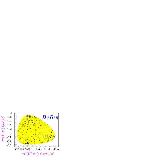
Figure 7: Dalitz plot of $D^{0}\rightarrow\overline{K}^{0}K^{+}\pi^{-}$.

The presence of the $K^{*+}(892)$ resonance is evident together with a small $K^{*0}(892)$ contribution with asymmetric lobes suggesting interference with other final states. A shoulder near the threshold of the $\overline{K}^{0}K^{+}$ mass distribution suggests the presence of the $a_{0}^{+}(980)$ resonance. This $D^{0}$ decay channel is fit using the final states shown in Table 6, which also displays the fit fractions and phases. The resulting $\chi^{2}$ for this fit is given in Table 4.

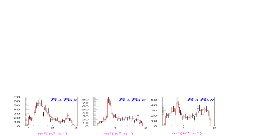
Figure 8: Dalitz plot projections for $D^{0}\rightarrow\overline{K}^{0}K^{+}\pi^{-}$. The data are represented with error bars; the histogram is a projection of the fit described in the text.

Table 6: Preliminary results from the Dalitz plot analysis of $D^{0}\rightarrow\overline{K}^{0}K^{+}\pi^{-}$.

Final state	Fraction (%)	Phase (degrees)
$K^{*0}_{0}(1430)\overline{K}^{0}$	26.0 $\pm$ 16.1 $\pm$ 3.3	–38 $\pm$ 22
$K^{*0}_{1}(892)\overline{K}^{0}$	2.8 $\pm$ 1.4 $\pm$ 0.5	–126 $\pm$ 19
$K^{*0}_{1}(1680)\overline{K}^{0}$	15.2 $\pm$ 11.9 $\pm$ 0.5	161 $\pm$ 9
$K^{*0}_{2}(1430)\overline{K}^{0}$	1.7 $\pm$ 2.5 $\pm$ 0.2	53 $\pm$ 38
$K^{*-}_{0}(1430)K^{+}$	2.4 $\pm$ 8.2 $\pm$ 1.0	–142 $\pm$ 115
$K^{*-}_{1}(892)K^{+}$	35.6 $\pm$ 7.7 $\pm$ 2.3	0
$K^{*-}_{1}(1680)K^{+}$	5.1 $\pm$ 5.7 $\pm$ 1.1	124 $\pm$ 27
$K^{*-}_{2}(1430)K^{+}$	1.0 $\pm$ 1.0 $\pm$ 0.2	–26 $\pm$ 38
$a_{0}^{+}(980)\pi^{-}$	15.1 $\pm$ 12.5 $\pm$ 0.6	-160 $\pm$ 42
$a_{0}^{+}(1450)\pi^{-}$	2.2 $\pm$ 2.7 $\pm$ 1.2	148 $\pm$ 25
N.R.	36.6 $\pm$ 25.8 $\pm$ 2.7	-172 $\pm$ 13
Sum	144 $\pm$ 37

This fit reveals a rather complex structure with large uncertainties due to the limited sample size. A sizeable nonresonant contribution is predicted by the fit, in contrast to the $D^{0}\rightarrow K^{0}K^{-}\pi^{+}$ channel discussed in the last section.

Dropping the nonresonant contribution results in a decrease of $2\log L$ of 9 units for 2 less parameters with the same $\chi^{2}$ value. While all other fractions have little changes, in this fit the contribution from $K^{*-}_{0}(1430)K^{+}$ increases from $(2\pm 8)$% to $(26\pm 12)$% and that of $a_{0}^{+}(980)\pi^{-}$ decreases from $(15\pm 13)$% to $(5\pm 6)$%. The sum of the fractions for this fit is (114 $\pm$ 23)%.

9 $D^{0}\rightarrow\overline{K}^{0}K^{+}K^{-}$ Dalitz Plot Analysis

The Dalitz plot for $D^{0}\rightarrow\overline{K}^{0}K^{+}K^{-}$ candidates is shown in Fig. 9 and its projections are shown in Fig. 10.

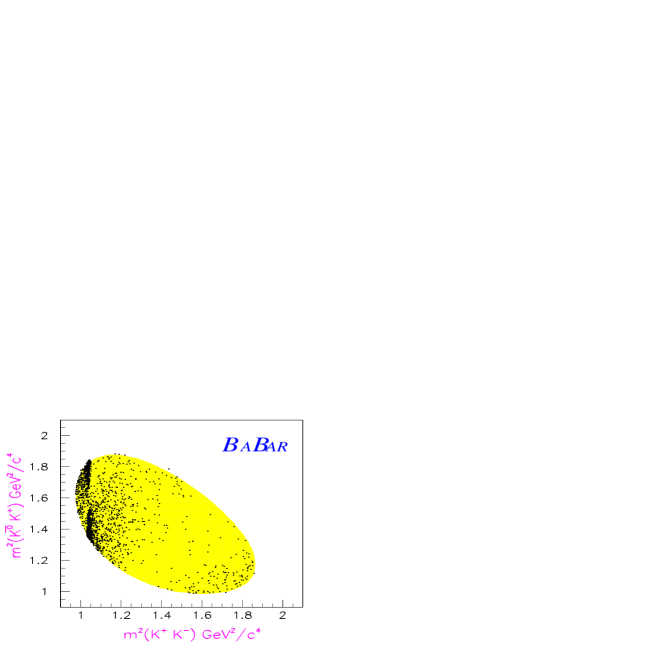
Figure 9: Dalitz plot of $D^{0}\rightarrow\overline{K}^{0}K^{+}K^{-}$.

A strong $\phi(1020)$ signal interfering with a threshold scalar meson can be clearly seen. Both $f_{0}(980)$ and $a_{0}^{0}(980)$ resonances can be present near threshold. An accumulation of events due to a charged $a_{0}^{+}(980)$ can be observed on the lower edge of the Dalitz plot. Table 7 shows the list of the final states and the fitted fractions and phases for this $D^{0}$ decay channel.

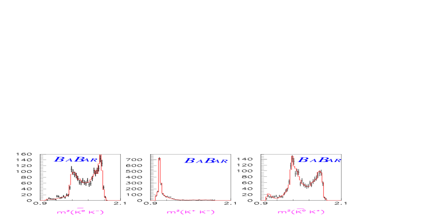
Figure 10: Dalitz plot projections for $D^{0}\rightarrow\overline{K}^{0}K^{+}K^{-}$. The data are represented with error bars; the histogram is the projection of the fit described in the text.

Table 7: Preliminary results from the Dalitz plot analysis of $D^{0}\rightarrow\overline{K}^{0}K^{+}K^{-}$.

Final state	Fraction (%)	Phase (degrees)
$\overline{K}^{0}\phi$	45.4 $\pm$ 1.6 $\pm$ 1.0	0
$\overline{K}^{0}a_{0}^{0}(980)$	60.9 $\pm$ 7.5 $\pm$ 13.3	109 $\pm$ 5
$\overline{K}^{0}f_{0}(980)$	12.2 $\pm$ 3.1 $\pm$ 8.6	–161 $\pm$ 14
$a_{0}(980)^{+}K^{-}$	34.3 $\pm$ 3.2 $\pm$ 6.8	–53 $\pm$ 4
$a_{0}(980)^{-}K^{+}$	3.2 $\pm$ 1.9 $\pm$ 0.5	-13 $\pm$ 15
N.R.	0.4 $\pm$ 0.3 $\pm$ 0.8	40 $\pm$ 44
Sum	156 $\pm$ 9

Most of the uncertainty in this channel is due to the poorly defined parameters of $a_{0}(980)$ and $f_{0}(980)$. Their properties are taken from measurements performed by other experiments. Since these states lie below $K\kern 1.99997pt\overline{\kern-1.99997ptK}{}$ threshold, their properties cannot be measured in this $D^{0}$ decay mode only. Their line shape would be best determined from a coupled-channel analysis of $K^{0}_{S}K^{0}_{S}$, $K^{0}_{S}K^{0}_{L}$, $K^{+}K^{-}$, $\eta\pi$ and $\pi\pi$ decays. A scan is made of the likelihood function with respect to the ratio $g_{K\kern 1.39998pt\overline{\kern-1.39998ptK}{}}/g_{\eta\pi}$ for $a_{0}(980)$ leaving the other parameters fixed. The likelihood has a maximum for $g_{K\kern 1.39998pt\overline{\kern-1.39998ptK}{}}/g_{\eta\pi}\sim$1.3, to be compared with the Crystal Barrel result of $1.01\pm 0.07$.

Similarly, a scan is performed as a function of $g_{K}/g_{\pi}$ for $f_{0}(980)$. The likelihood has a maximum for $g_{K}/g_{\pi}\sim$1.25, to be compared with the WA76 result of $2.0\pm 0.6$. The variation of the fractions due to the change of these parameters is taken into account in the evaluation of the systematic errors.

The doubly-Cabibbo-suppressed contribution $D^{0}\rightarrow K^{0}K^{+}K^{-}$ has also been included in the fit. The presence of such a contribution should show up as an $a_{0}^{-}(980)$ signal in the $K^{0}K^{-}$ effective mass. The insertion of this new term results in an increase of $2\log L$ by 10 units for 2 additional parameters and the resulting $\chi^{2}$ is included in Table 4. However, with the present statistics, its contribution of (3.2 $\pm$ 1.9)% is consistent with zero.

The poor fit quality for this channel, indicated by the $\chi^{2}/N_{cells}$ of $98/59$ in Table 4, comes mostly from the $\phi$ mass region. Effects of $\phi$ mass resolution comparable to its natural width combined with uncertainties in the $a_{0}$ and $f_{0}$ line shapes are not included in the current fit model, and do not correctly model the interference in this region. Future analyses with larger data samples should attempt to address this problem with a more detailed model.

10 Summary

Dalitz plot analyses are performed for the hadronic decays $D^{0}\rightarrow K^{0}K^{-}\pi^{+}$, $D^{0}\rightarrow\overline{K}^{0}K^{+}\pi^{-}$ and $D^{0}\rightarrow\overline{K}^{0}K^{+}K^{-}$. The fractions and relative phases for intermediate resonant states are extracted. The following preliminary ratios of branching fractions are measured:

$$\frac{D^{0}\rightarrow K^{0}K^{-}\pi^{+}}{D^{0}\rightarrow\overline{K}^{0}\pi^{+}\pi^{-}}=(8.32\pm 0.29(stat)\pm 0.56(syst))\times 10^{-2},$$

$$\frac{D^{0}\rightarrow\overline{K}^{0}K^{+}\pi^{-}}{D^{0}\rightarrow\overline{K}^{0}\pi^{+}\pi^{-}}=(5.68\pm 0.25(stat)\pm 0.41(syst))\times 10^{-2},$$

$$\frac{D^{0}\rightarrow\overline{K}^{0}K^{+}K^{-}}{D^{0}\rightarrow\overline{K}^{0}\pi^{+}\pi^{-}}=(16.30\pm 0.37(stat)\pm 0.27(syst))\times 10^{-2}.$$

11 Acknowledgments

We are grateful for the extraordinary contributions of our PEP-II colleagues in achieving the excellent luminosity and machine conditions that have made this work possible. The success of this project also relies critically on the expertise and dedication of the computing organizations that support BABAR. The collaborating institutions wish to thank SLAC for its support and the kind hospitality extended to them. This work is supported by the US Department of Energy and National Science Foundation, the Natural Sciences and Engineering Research Council (Canada), Institute of High Energy Physics (China), the Commissariat à l’Energie Atomique and Institut National de Physique Nucléaire et de Physique des Particules (France), the Bundesministerium für Bildung und Forschung and Deutsche Forschungsgemeinschaft (Germany), the Istituto Nazionale di Fisica Nucleare (Italy), the Research Council of Norway, the Ministry of Science and Technology of the Russian Federation, and the Particle Physics and Astronomy Research Council (United Kingdom). Individuals have received support from the A. P. Sloan Foundation, the Research Corporation, and the Alexander von Humboldt Foundation.

References

- [1] M. Bauer et al., Z. Phys. C34 (1987) 103.
- [2] C. Gobel et al., in proceedings of the IX International Conference on Hadron Spectroscopy, edited by D. Amelin, AIP, 2001.
- [3] B. Aubert et al., Nucl. Instrum. Methods A479 (2002) 1.
- [4] GEANT, CERN Program Library, Long Writeup W5013 (1994).
- [5] D.E. Groom et al., The European Physical Journal, C15 (2000) 1.
- [6] R. Ammar et al., Phys. Rev. D44 (1991) 3383.
- [7] H. Albrecht et al., Z. Phys. C46 (1990) 9.
- [8] J.C. Anjos et al., Phyd. Rev. D43 (1991) R635.
- [9] H. Albrecht et al., Phys. Lett. B 308 (1993) 435.
- [10] S. Kopp et al., Phys. Rev. D63 (2001) 092001.
-
[11]
C. Zemach, Phys. Rev. 133 B (1964) 1201;
C. Zemach, Phys. Rev. 140 B (1965) 97. - [12] C. Amsler et al., Phys. Lett. B 311 (1993) 362.
- [13] T.A. Armstrong et al., Z. Phys. C51 (1991) 351.
- [14] A. Abele et al., Phys. Rev. D57 (1998) 3860.
-
[15]
D. Aston et al., Nucl. Phys. B296 (1988) 493;
D. Aston, B. Dunwoodie, private communication. -
[16]
R. Jaffe, Phys. Rev. D15 (1977) 267;
R. Jaffe, Phys. Rev. D15 (1977) 281;
M.D. Scadron, Phys. Rev. D26 (1982) 239.