The BABAR Collaboration

July 25, 2002

Abstract

We present a preliminary measurement of the branching fraction for $B\rightarrow\rho e\nu$ and of the CKM matrix element $|V_{ub}|$ using approximately $55$ million $B\bar{B}$ meson pairs collected with the BABAR detector. Using isospin relations for several modes we find

$${\cal B}(B^{0}\rightarrow~{}\rho^{-}~{}e^{+}~{}\nu) = (3.39~{}\pm~{}0.44~{}\pm~{}{0.52}\pm~{}0.60)~{}\times 10^{-4}$$

$$|V_{ub}| = (3.69~{}\pm~{}0.23~{}\pm~{}0.27~{}{}^{+0.40}_{-0.59})~{}\times~{}10^{-3}.$$

The quoted errors are statistical, systematic, and theoretical respectively. These results are obtained by using five different form-factor calculations.

1 Introduction

Exclusive $b\rightarrow u\ell\nu$ decays can be used to determine the modulus of $V_{ub}$, one of the smallest and least well known CKM matrix elements. Compared to the determination with inclusive decays, the extra kinematical constraints allow access to a larger part of the lepton-momentum spectrum, resulting in smaller extrapolation uncertainties. Experimentally, the main difficulty for the observation of $b\rightarrow u\ell\nu$ signal events is the large background from $b\rightarrow c\ell\nu$ events. Because $|V_{ub}/V_{cb}|\approx 0.1$, the branching fractions of the exclusive $b\rightarrow u\ell\nu$ decays ($\sim 10^{-4}$) are small compared to those of the charmed semileptonic decays, which are of the order of some percent.

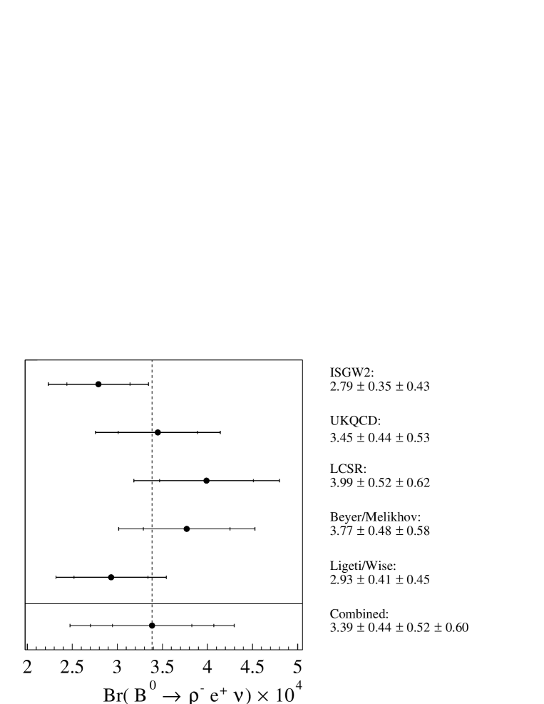
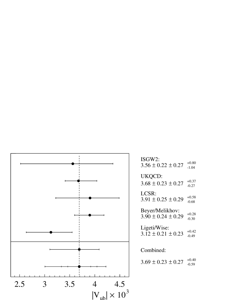
To extract the branching fraction $B\rightarrow\rho e\nu$ and $|V_{ub}|$ requires use of hadronic form-factors which have to be obtained from theory. In this analysis we use five different form factor calculations: the two quark models ISGW2 [1] and Beyer/Melikhov [2], the lattice calculation by the UKQCD group [3], a model based on light cone sum rules (LCSR [4]), and a model based on heavy quark and $SU(3)$ symmetries (Ligeti/Wise [5]). The UKQCD and LCSR calculations directly use QCD, whereas the quark models are more phenomenological. All calculations use a particular value of $q^{2}=(p_{e}+p_{\nu})^{2}$ as a normalization point. Usually, $q^{2}_{\rm max}$ is used as this is the point where the hadronic system is least disturbed. The LCSR result however is normalized at a lower value of $q^{2}$.

2 The BABAR Detector and Data Set

The data used in this analysis were collected with the BABAR detector [6] at the PEP-II $e^{+}e^{-}$ storage ring [7]. The integrated luminosity of the sample is $50.5\mbox{\,fb}^{-1}$ taken at the $\mathchar 28935\relax{(4S)}$ mass (“on-resonance”), corresponding to $55.2$ million $B\bar{B}$ meson pairs. An additional $8.7\mbox{\,fb}^{-1}$ of data were taken $40\mathrm{\,Me\kern-1.00006ptV}$ below the $\mathchar 28935\relax{(4S)}$ resonance (“off-resonance”).

PEP-II is an $e^{+}e^{-}$ collider operated with asymmetric beam energies, producing a boosted ($\beta\gamma=0.55$) $\mathchar 28935\relax{(4S)}$ along the collision axis. BABAR is a solenoidal detector optimized for the asymmetric beam configuration at PEP-II. Charged particle (track) momenta are measured in a tracking system consisting of a 5-layer, double-sided, silicon vertex tracker (SVT) and a 40-layer drift chamber (DCH) filled with a gas mixture of helium and isobutane, both operating within a $1.5\,{\rm T}$ superconducting solenoidal magnet. Photon candidates are selected as local maxima of deposited energy in an electromagnetic calorimeter (EMC) consisting of 6580 CsI(Tl) crystals arranged in barrel and forward endcap subdetectors. Particle identification is performed by combining information from ionization measurements ($\mathrm{d}E/\mathrm{d}x$) in the SVT and DCH, and the Cherenkov angle $\theta_{c}$ measured by a detector of internally reflected Cherenkov light (DIRC). The DIRC system is a unique type of Cherenkov detector that relies on total internal reflection within the radiating volumes (quartz bars) to deliver the Cherenkov light outside the tracking and magnetic volumes, where the Cherenkov ring is imaged by an array of $\sim 11000$ photomultiplier tubes. The detector is surrounded by an instrumented flux-return (IFR).

3 Event Selection

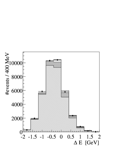
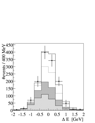
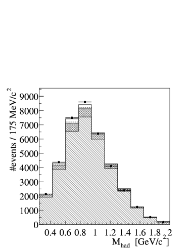
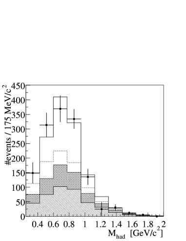
In this section, we describe the selection of the exclusive semileptonic decays $B^{+}\rightarrow\rho^{0}e^{+}\nu$,  $B^{0}\rightarrow\rho^{-}e^{+}\nu$,  $B^{+}\rightarrow\omega e^{+}\nu$,  $B^{+}\rightarrow\pi^{0}e^{+}\nu$,  and $B^{0}\rightarrow\pi^{-}e^{+}\nu$  (with $\rho^{0}\rightarrow\pi^{+}\pi^{-}$, $\rho^{\pm}\rightarrow\pi^{0}\pi^{\pm}$ and $\omega\rightarrow\pi^{0}\pi^{+}\pi^{-}$). The charge conjugate decays are implied throughout. Our analysis strategy is similar to one used by CLEO [8]. The analysis is optimized for $B\rightarrow\rho e\nu$ decays; the $\pi$ and $\omega$ modes are included because of the crossfeeds into the $\rho$ modes. Isospin and quark model relations are used to effectively measure only two branching fractions, one for $B\rightarrow\rho e\nu$ and one for $B\rightarrow\pi e\nu$. This is described in section 4. This analysis uses only electrons and not muons because the background contribution from fake leptons is much lower in the case of electrons. We reconstruct three kinematic variables which are used in the fit to extract the signal yields. These are the electron energy $E_{\rm lept}^{\rm CM}$, the invariant hadronic mass $M_{\pi\pi(\pi)}$ (for the $\rho$ and $\omega$ modes), and the difference between the reconstructed and expected $B$ meson energy ($\Delta E\equiv E_{\rm hadron}+E_{\ell}+|{\vec{p}}_{{\rm miss}}|c-E_{\rm beam}$) in the center-of-mass (CM) system.

Two electron energy regions are considered: $2.0\leq E^{\rm CM}_{\rm lept}<2.3\mbox{ GeV}$ (LOLEP), and $2.3\leq E^{\rm CM}_{\rm lept}<2.7\mbox{ GeV}$ (HILEP). The HILEP region is most sensitive to the signal because the $b\rightarrow ce\nu$ events are almost completely suppressed; the largest background source here is from continuum $e^{+}e^{-}\rightarrow q\bar{q}$ events. Real data taken below the $\mathchar 28935\relax(4S)$ mass, which includes $e^{+}e^{-}\rightarrow e^{+}e^{-}(\gamma)$ events, is used for the continuum subtraction. In the LOLEP region, $b\rightarrow c$ decays dominate and provide the normalization of the background at higher electron energies.

Hadronic events are selected based on track multiplicity and event topology. The tracks must have at least 12 hits in the drift chamber. We also require that the impact parameter of the track along and transverse to the beam direction must be less than 3 cm and 1 cm, respectively. In addition, the transverse momentum must be greater than $0.1\mbox{ GeV}/c$. Clusters in the electromagnetic calorimeter of BABAR that are not associated to any tracks must have an energy greater than $30\mbox{ MeV}$ to be considered as photons. In addition, the lateral moment of the shower energy distribution [10] must be smaller than $0.8$. We select events with either $N_{\rm tracks}\geq 5$ or ($N_{\rm tracks}\geq 4$ and $N_{\rm photons}\geq 5$). The $B$ mesons are produced nearly at rest so their decay products are distributed roughly uniformly in solid angle. In contrast, continuum events have a much more collimated (jet-like) event topology. They are suppressed by requiring the ratio of Fox-Wolfram moments $H_{2}/H_{0}$ [9] to be less than 0.4. This requirement suppresses 55% of the $e^{+}e^{-}\rightarrow q\bar{q}$ background and non-hadronic events, with a signal efficiency of 85%. In addition a neural net is used for further suppression of continuum events, as described below.

To identify electrons, we use a likelihood estimator, which uses information from several BABAR sub-detectors. The primary information is the ratio of the calorimeter energy to the track momentum. We require that the direction of the electron momentum is within the good calorimeter acceptance $-0.72<\cos\theta_{e,{\rm lab}}<0.92$. The efficiency of this selector is around $90\%$, with a pion misidentification rate of less than $0.1\%$. We also reject electrons from $J/\psi$ decays (requiring two electrons identified with the likelihood electron selector and $3.00<M_{e^{+}e^{-}}<3.14\mbox{ GeV}/c^{2}$) and from photon conversions ($M_{e^{+}e^{-}}<30\mbox{ MeV}/c^{2}$).

To reconstruct the neutral $\rho$ meson we combine two oppositely charged tracks, and for the case of the charged $\rho$ a track and a $\pi^{0}$. The $\pi^{0}$ mesons are reconstructed from two photons with an invariant mass $120<M_{\gamma\gamma}<145\mbox{ MeV}/c^{2}$ corresponding to $\pm 2\ \sigma$ from the nominal $\pi^{0}$ mass on average. To suppress combinatorial backgrounds we require that the pion with the highest momentum must have $p_{\pi}^{\rm CM}>400\mbox{ MeV}/c$ and the other pion must satisfy $p_{\pi}^{\rm CM}>200\mbox{ MeV}/c$. For the $\omega$, we combine two oppositely charged tracks with a $\pi^{0}$. The $\omega$ invariant mass is measured within $\pm 80\mbox{ MeV}/c^{2}$ of the nominal $\omega$ mass [11]. This includes a side band region below and above the nominal $\omega$ mass. To suppress combinatorial backgrounds we require $p_{\pi}^{\rm CM}>100\mbox{ MeV}/c$ for each of the three pions. The charged tracks used to reconstruct the $rho$, $omega$, or $pi^{\pm}$ mesons must not have been identified as kaons.

In the following discussion all variables are taken in the center-of-mass frame. The neutrino is reconstructed from the missing momentum:

$$\vec{p}_{\rm miss}=-\sum_{\rm tracks}{\vec{p}_{i}}-\sum_{\rm photons}{\vec{p}_{i}}\;,$$ (1)

where the sums run over all reconstructed and accepted tracks and photons in the event. We then take $(E_{\nu},\vec{p}_{\nu})=(|\vec{p}_{\rm miss}|c,\vec{p}_{\rm miss})$.

Figure 1: Angles $\theta_{BY}$ and $\Delta\theta$ defined in the $\mathchar 28935\relax(4S)$ frame.

A $B$-meson decay consistent with the signal modes is reconstructed using the constraints $E_{B}=E_{\rm beam}$ and $(p_{B}-p_{Y})^{2}=0$, where $Y$ is the $(\rho,~{}\omega,~{}\pi)+e$ system. A useful quantity for testing consistency is the angle between the $B$ momentum direction and that of the reconstructed $Y$ system, see Fig. 1,

$$\cos\theta_{BY}={2E_{B}E_{Y}-(M_{B}^{2}+M_{Y}^{2})c^{4}\over 2|\vec{p}_{B}||\vec{p}_{Y}|c^{2}}\;.$$ (2)

Background tends to have non-physical values of $\cos\theta_{BY}$. For the signal, small extensions of $|\cos\theta_{BY}|>1$ are allowed because of detector resolution. We therefore require

$$|\cos\theta_{BY}|<1.1\;.$$ (3)

The efficiency of this requirement is almost 100% for the signal and it rejects more than 60% of the $b\rightarrow ce\nu$ and 80% of the continuum background.

We also compare the direction of the missing momentum $\vec{p}_{{\rm miss}}$ with that of the neutrino momentum inferred from $\vec{p}_{\nu}=\vec{p}_{B}-\vec{p}_{Y}$. The latter is known to within an azimuthal ambiguity about the $\vec{p}_{B}$ direction because the magnitude, but not the direction, of the $B$ meson momentum is known. We use the smallest possible angle $\Delta\theta_{\rm min}$ between the two directions, which is obtained when the momenta of $\vec{p}_{Y}$, $\vec{p}_{\nu}$, and $\vec{p}_{\rm miss}$ are in the same plane, see Fig. 1. We use the requirement

$$0.8<\cos\Delta\theta_{\rm min}\leq 1.0\;.$$ (4)

This has been optimized using a Monte Carlo simulation, in such a way as to minimize the relative error on the measured branching fraction.

In addition, we require $|\cos\theta_{{\rm miss}}|<0.9$ where $\theta_{\rm miss}$ is the angle between $\vec{p}_{\rm miss}$ and the beam axis. This cut rejects events with missing high momentum particles close to the beam axis.

The continuum $e^{+}e^{-}\rightarrow q\bar{q}$, where $q=u,d,s,c$, is an important background at high electron energies, where we are most sensitive to the signal. To reject these events, we use a neural net with 14 event shape variables such as the track and cluster energies in nine cones around the electron-momentum axis. The optimized cut on the neural net output suppresses more than 90% of the continuum, after all other requirements have been applied, in the HILEP region. The selection efficiency on the signal is 60%.

After all the above criteria, there can still be several candidates per event. This follows from the large width of the $\rho$ and also because we are reconstructing five different decay modes. To avoid statistical difficulties related to large numbers of combinations, we choose one candidate per event, namely the one with a reconstructed total momentum closest to the B meson momentum:

$$|\vec{p}_{\rm hadron}+\vec{p}_{e}+\vec{p}_{\rm miss}|\;\;{\rm closest\;to}\;\;|\vec{p}_{B}|.$$ (5)

The efficiency of this selection for the signal is close to 85% .

At each step of the selection procedure the data distributions agree well with their Monte Carlo simulation.

The total efficiencies in the HILEP region are $4.21\%$ for the $B^{+}\rightarrow\rho^{0}e^{+}\nu$ mode and $3.31\%$ for the $B^{0}\rightarrow\rho^{-}e^{+}\nu$ mode. These efficiencies are determined using the ISGW2 form-factors. They are defined here as the number of HILEP signal events that pass all selection criteria and are reconstructed in the specified channel divided by the number of all generated events (of all electron momenta) for this channel. The signal and crossfeed efficiencies for all channels are listed in Table 1.

Table 1: Selection efficiencies for the modes $B^{+}\rightarrow\rho^{0}e^{+}\nu$, $B^{0}\rightarrow\rho^{-}e^{+}\nu$, $B^{+}\rightarrow\omega e^{+}\nu$, $B^{+}\rightarrow\pi^{0}e^{+}\nu$, and $B^{0}\rightarrow\pi^{-}e^{+}\nu$ in the HILEP region. These efficiencies have been determined using simulated data (ISGW2 model). They are defined as the number of selected events passing all cuts divided by the number of all generated events (in the full lepton energy range) for the specified channel.

	Reconstruction Efficiency (%)
Generated	$B^{+}\rightarrow\rho^{0}e^{+}\nu$	$B^{0}\rightarrow\rho^{-}e^{+}\nu$	$B^{+}\rightarrow\omega e^{+}\nu$	$B^{+}\rightarrow\pi^{0}e^{+}\nu$	$B^{0}\rightarrow\pi^{-}e^{+}\nu$
$B^{+}\rightarrow\rho^{0}e^{+}\nu$	$4.21$	$0.99$	$0.30$	$0.58$	$1.35$
$B^{0}\rightarrow\rho^{-}e^{+}\nu$	$1.04$	$3.31$	$0.31$	$1.08$	$1.32$
$B^{+}\rightarrow\omega e^{+}\nu$	$1.97$	$1.55$	$1.57$	$0.94$	$0.88$
$B^{+}\rightarrow\pi^{0}e^{+}\nu$	$0.23$	$0.41$	$0.07$	$1.28$	$0.40$
$B^{0}\rightarrow\pi^{-}e^{+}\nu$	$0.42$	$0.47$	$0.05$	$0.33$	$1.63$

4 Fit Method

We have performed a binned maximum-likelihood fit of the two-dimensional distribution ($M_{\pi\pi(\pi)}$, $\Delta E$) simultaneously in the two electron energy ranges (LOLEP, HILEP) and the decay modes $B^{+}\rightarrow\rho^{0}e^{+}\nu$,  $B^{0}\rightarrow\rho^{-}e^{+}\nu$,  and $B^{+}\rightarrow\omega e^{+}\nu$. For the $B\rightarrow\rho e\nu$ modes, the data are divided into $10\times 10$ bins over the ($M_{\pi\pi}$, $\Delta E$) region $0.25\leq M_{\pi\pi}\leq 2.00\mbox{ GeV}/c^{2}$ and $|\Delta E|\leq 2\mbox{ GeV}$. The bin size for the fit is thus $175\mbox{ MeV}/c^{2}$ in $M_{\pi\pi}$ and $400\mbox{ MeV}$ in $\Delta E$. For the $\omega$ channel, we use 5 bins in the range $782\pm 80\mbox{ MeV}/c^{2}$ and 10 bins in $|\Delta E|\leq 2\mbox{ GeV}$. The modes $B^{+}\rightarrow\pi^{0}e^{+}\nu$  and $B^{0}\rightarrow\pi^{-}e^{+}\nu$  are also included to model the crossfeeds into the other signal channels; for these modes only $\Delta E$ is used as a fit variable.

Our fit includes contributions from the signal modes, other $b\rightarrow ue\nu$ decays, $b\rightarrow ce\nu$ decays, continuum, and a contribution from misidentified electrons. For the signal and backgrounds coming from other $b\rightarrow ue\nu$ and $b\rightarrow ce\nu$ decays, Monte Carlo simulation provides the shapes of the distributions. The decays $B\rightarrow D^{*}\ell\nu$ have been simulated using heavy quark effective theory (HQET [12]). The modes $B\rightarrow D^{*}\pi\ell\nu$ are simulated according to the Goity-Roberts model [13]. Resonant $b\rightarrow u\ell\nu$ downfeed modes are implemented according to the ISGW2 model. Non-resonant $b\rightarrow u\ell\nu$ modes are implemented according to a model by Fazio and Neubert [14].

Isospin and quark model relations are used to constrain the relative normalizations of $B^{0}\rightarrow\rho^{-}e^{+}\nu$, $B^{+}\rightarrow\rho^{0}e^{+}\nu$, and $B^{+}\rightarrow\omega e^{+}\nu$ and therefore to reduce the number of free fit parameters:

$$\Gamma(B^{0}\rightarrow\rho^{-}e^{+}\nu) = 2\Gamma(B^{+}\rightarrow\rho^{0}e^{+}\nu),$$ (6)

$$\Gamma(B^{+}\rightarrow\rho^{0}e^{+}\nu) = \Gamma(B^{+}\rightarrow\omega e^{+}\nu),$$ (7)

$$\Gamma(B^{0}\rightarrow\pi^{-}e^{+}\nu) = 2\Gamma(B^{+}\rightarrow\pi^{0}e^{+}\nu).$$ (8)

Isospin breaking effects are discussed in [15] and [16]. We assume that the isospin relations in Eqs. 6 and 7 are broken by not more than $3\%$. This would have a negligible effect on our result and therefore we do not include a corresponding systematic error. The isospin relations were tested experimentally. We find that the isospin relations Eqs. 6 and 7 are consistent with the data within $1.3\;\sigma$ and $1.7\;\sigma$.

We use the following 9 free parameters for the fit:

• ${\cal B}(B^{0}\rightarrow\rho^{-}e^{+}\nu)$ (1 parameter);

• ${\cal B}(B^{0}\rightarrow\pi^{-}e^{+}\nu)$ (1 parameter);

• the scale factors of the $b\rightarrow ue\nu$ background in each electron energy bin (2 parameters), that give the overall normalization of all $b\rightarrow ue\nu$ modes that are not signal modes, relative to that expected from the Monte Carlo simulation;

• the scale factors, one for each mode, that give the overall normalization of the $b\rightarrow ce\nu$ background relative to that expected from the Monte Carlo simulation (5 parameters).

The maximum-likelihood fit method used in this analysis has been described in [17]. The fit takes into account the statistical fluctuations not only of the on-resonance and off-resonance data but also those of the Monte Carlo contributions. We have performed a toy Monte Carlo check to verify the stability of the fit method and to check the statistical error returned by the fit.

Whereas the signal modes $B^{+}\rightarrow\rho^{0}e^{+}\nu$, $B^{0}\rightarrow\rho^{-}e^{+}\nu$, and $B^{+}\rightarrow\omega e^{+}\nu$  are simulated with five different form-factors, all other $b\rightarrow ue\nu$ modes (downfeed background) are simulated using the ISGW2 form-factor only.

5 Fit Results

Table 2: Summary of data yields for the $B^{0}\rightarrow\rho^{-}e^{+}\nu$  and $B^{+}\rightarrow\rho^{0}e^{+}\nu$  modes with electron energies between $2.3$ and $2.7\mbox{ GeV}$ (HILEP), and between $2.0$ and $2.3\mbox{ GeV}$ (LOLEP). The yields presented in this table were obtained using the ISGW2 form-factor. The downfeed background includes all $B\rightarrow X_{u}e\nu$ modes except for $\rho$, $\omega$, and $\pi$. The crossfeed signal contribution corresponds to events from the other signal modes with $\rho^{0}$, $\omega$, or $\pi$ and is constrained to the signal in the fit. All errors are statistical only.

	$B^{0}\rightarrow\rho^{-}e^{+}\nu$		$B^{+}\rightarrow\rho^{0}e^{+}\nu$
	HILEP	LOLEP	HILEP	LOLEP
On-resonance yield	2302	39349	2213	40155
Direct signal	510 $\pm$ 63	718 $\pm$ 89	324 $\pm$ 40	440 $\pm$ 55
Crossfeed signal	262 $\pm$ 32	538 $\pm$ 73	363 $\pm$ 42	725 $\pm$ 86
Downfeed	203 $\pm$ 55	2278 $\pm$ 403	226 $\pm$ 92	2435 $\pm$ 430
$b\rightarrow ce\nu$	414 $\pm$ 5	33859 $\pm$ 438	367 $\pm$ 5	34366 $\pm$ 458
$e^{+}e^{-}\rightarrow q\bar{q}$	917 $\pm$ 73	1928 $\pm$ 106	912 $\pm$ 73	2063 $\pm$ 110
Fake electrons	12 $\pm$ 3	80 $\pm$ 9	18 $\pm$ 4	76 $\pm$ 9

The signal yields extracted from the binned maximum-likelihood fit in the HILEP region are 324 $\pm$ 40 $B^{+}\rightarrow\rho^{0}e^{+}\nu$  events and 510 $\pm$ 63 $B^{0}\rightarrow\rho^{-}e^{+}\nu$  events, based on the ISGW2 calculation. The composition of events for the $B^{0}\rightarrow\rho^{-}e\nu$ and $B^{+}\rightarrow\rho^{0}e^{+}\nu$ channel is shown in Table 2. The isospin-constrained results for the five different form-factors are shown in Fig. 2. A $\chi^{2}$ test has been performed to check the quality of the fit. Bins in sparsely populated regions have been combined before the $\chi^{2}$ calculation. For ISGW2, we obtain $\chi^{2}=91$ for $N_{\rm dof}=93$, which corresponds to a $p$-value of $0.52$, and similarly good fit quality for the other four form-factor calculations.

The five fit parameters describing the $b\rightarrow c$ backgrounds agree with the Monte Carlo expectations within $9\%$ on average. The two parameters describing the $b\rightarrow u$ downfeed background in LOLEP and HILEP agree to better than $1.5\ \sigma$ and $1.2\ \sigma$. The fit result for the $\pi$ modes is ${\cal B}(B^{0}\rightarrow\pi^{-}e^{+}\nu)=(1.87\pm 0.56)\times 10^{-4}$ for the ISGW2 calculation.

Figure 2: The $B^{0}\rightarrow\rho^{-}e^{+}\nu$  branching fraction results using the ISGW2, UKQCD, LCSR, Beyer/Melikhov, and Ligeti/Wise form-factors. The errors shown are statistical, systematic, and (only in case of the combined result) theoretical, successively combined in quadrature. The combined central value is determined by taking the unweighted mean of all form-factor results. The statistical and systematic errors of the combined result are determined by taking the means of the relative errors of each individual result, and its theoretical error is taken to be one half of the full spread of the results.

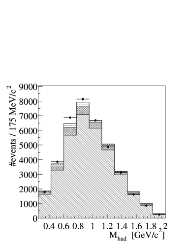
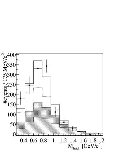
The projections of the ISGW2 fit result for the two electron energy bins after subtraction of the continuum contribution are shown in Figs. 3 and 4. Good agreement between the data and fit result is seen in each of these figures. The fits for the other four form-factor calculations show similar agreement.

(a) $M_{\pi\pi}$ (LOLEP)

(b) $M_{\pi\pi}$ (HILEP)

(c) $\Delta E$ (LOLEP)

(d) $\Delta E$ (HILEP)

Figure 3: Continuum-subtracted projections of the ISGW2 fit result for the $B^{+}\rightarrow\rho^{0}e^{+}\nu$ channels in the LOLEP and HILEP electron energy regions; the contributions are the direct and crossfeed components of the signal (unhatched region, above and below the dashed line, respectively); the background from $b\rightarrow ue\nu$ other than $B\rightarrow\rho e\nu$ and $B\rightarrow\omega e\nu$ modes (double-hatched region); the background from $b\rightarrow ce\nu$ and other backgrounds (single-hatched region).

(a) $M_{\pi\pi}$ (LOLEP)

(b) $M_{\pi\pi}$ (HILEP)

(c) $\Delta E$ (LOLEP)

(d) $\Delta E$ (HILEP)

Figure 4: Continuum-subtracted projections of the ISGW2 fit result for the $B^{0}\rightarrow\rho^{-}e^{+}\nu$ channels in the LOLEP and HILEP electron energy regions; the contributions are the direct and crossfeed components of the signal (unhatched region, above and below the dashed line, respectively); the background from $b\rightarrow ue\nu$ other than $B\rightarrow\rho e\nu$ and $B\rightarrow\omega e\nu$ modes (double-hatched region); the background from $b\rightarrow ce\nu$ and other backgrounds (single-hatched region).

6 Systematic Errors

The summary of all systematic errors on the branching fraction that have been considered is shown in Table 3. The total systematic error is taken as the quadratic sum of all individual errors. The fluctuations due to finite Monte Carlo statistics are included in the statistical error and not in the systematic error.

The largest single systematic error comes from the uncertainty in the shape of the downfeed background. We use the ISGW2 model to describe resonant downfeed modes, and a model by Fazio and Neubert [14] for non-resonant modes. The fraction of non-resonant events in the downfeed background is varied from $0\%$ to $68\%$ to estimate this systematic uncertainty. The composition of the resonant $b\rightarrow u$ downfeed component has been varied by changing the branching fraction for individual resonances by $\pm 50\%$, and keeping the total rate constant.

We have also varied the most important selection requirements of this analysis within a reasonable range and have changed our fit method (fitting with only four channels, or without the LOLEP region, or with different binnings). Most variations seen are within $1\sigma$ of the expected statistical variation, some are close to $2\sigma$. To be conservative we assign a systematic error corresponding to half the largest variations seen. This corresponds to the last two systematic errors quoted in Table 3.

Table 3: Summary of all contributions to the systematic error on the branching fraction for $B\rightarrow\rho e\nu$.

Error contribution	$\delta{\cal B}_{\rho}/{\cal B}_{\rho}$ (%)
Tracking Efficiency	$\pm 5$
Tracking Resolution	$\pm 1$
Photon/$\pi^{0}$ Efficiency	$\pm 5$
Photon/$\pi^{0}$ Energy Scale	$\pm 3$
$b\rightarrow c$ Background Composition	${}^{+1.4}_{-1.7}$
Resonant $b\rightarrow u$ Background Composition	${}^{+6}_{-4}$
Non-Resonant $b\rightarrow u$ Background	$\pm 9$
B Lifetime	$\pm 1$
B Counting	$\pm 1.6$
Fake Electrons	$<\pm 1$
Electron Id	$\pm 2$
$f_{\pm}/f_{00}$	$<\pm 1$
Data Selection	$\pm 6$
Fit Method	${}^{+4}_{-6}$
Total Systematic Error	$\pm 15.5$

7 Extraction of $|V_{ub}|$

Table 4: $\tilde{\Gamma}_{{\rm thy}}$ predicted by various form-factor calculations.

Form-factor	$\tilde{\Gamma}_{{\rm thy}}$ (ps-1)	Estimated error on $\tilde{\Gamma}_{{\rm thy}}(\%)$
ISGW2	14.2	$\pm 50$
LCSR	16.9	$\pm 32$
UKQCD	16.5	${}^{+21}_{-14}$
Beyer/Melikhov	16.0	$\pm 15$
Ligeti/Wise	19.4	$\pm 29$

The CKM matrix element $|V_{ub}|$ can be obtained from the branching fraction ${\cal B}(B^{0}\rightarrow\rho^{-}e^{+}\nu)$ using

$$|V_{ub}|=\sqrt{{{\cal B}(B^{0}\rightarrow\rho^{-}e^{+}\nu)\over{\tilde{\Gamma}_{{\rm thy}}\tau_{B^{0}}}}}\;,$$ (9)

where $\tilde{\Gamma}_{{\rm thy}}$ is the predicted form-factor normalization. Values of $\tilde{\Gamma}_{{\rm thy}}$ and theoretical errors for each form-factor calculation are given in Table 4. The calculations quote errors on $\tilde{\Gamma}_{{\rm thy}}$ between $15\%$ and $50\%$. We use $\tau_{B^{0}}=1.548\pm 0.032$ ps [11], and the branching fractions are taken separately for each form-factor as listed in Fig. 2. The combined central value is determined by taking the weighted mean of all form-factor results. The statistical and systematic errors of the final combined result are determined by taking the mean of the relative errors of each individual result. The theoretical error is taken to be one half of the full spread of all fit results (including theoretical errors). The results for each form-factor and the combined result is shown in Fig. 5.

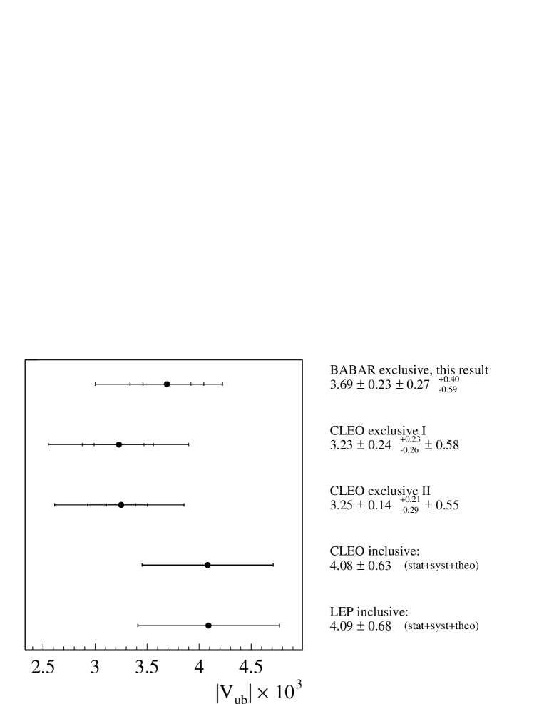
A comparison of our preliminary result with inclusive and exclusive measurements from CLEO and the inclusive measurement from LEP is shown in Fig. 6. Two exclusive results from CLEO are quoted. The first result is obtained from an analysis very similar to the analysis presented here [8], the second result is an average of their first result and a separate analysis [8, 18]. Our result is compatible with all other measurements within errors and lies between the CLEO and LEP results.

Figure 5: $|V_{ub}|$ determined using the ISGW2, UKQCD, LCSR, Beyer/Melikhov, and Ligeti/Wise form-factors. The results for each form-factor are drawn with theoretical error bars only. The combined central value is determined by taking the mean of all form-factor results, weighted by their individual theoretical error. The theoretical error of the combined result is taken to be one half of the full spread of results, including the errors. The combined result is also drawn with statistical, systematic, and theoretical errors successively added in quadrature. The statistical and systematic errors of the combined result are determined by taking the mean of the relative errors of each individual result. In addition we give, on the right side of the figure, all five results with their statistical, systematic, and theoretical errors.

Figure 6: Comparison with results from other experiments. The CLEO exclusive I result [8] is obtained from an analysis very similar to the analysis presented here, their exclusive II result [18] is an average of the exclusive I result and a separate CLEO result.

8 Acknowledgements

We are grateful for the extraordinary contributions of our PEP-II colleagues in achieving the excellent luminosity and machine conditions that have made this work possible. The success of this project also relies critically on the expertise and dedication of the computing organizations that support BABAR. The collaborating institutions wish to thank SLAC for its support and the kind hospitality extended to them. This work is supported by the US Department of Energy and National Science Foundation, the Natural Sciences and Engineering Research Council (Canada), Institute of High Energy Physics (China), the Commissariat à l’Energie Atomique and Institut National de Physique Nucléaire et de Physique des Particules (France), the Bundesministerium für Bildung und Forschung and Deutsche Forschungsgemeinschaft (Germany), the Istituto Nazionale di Fisica Nucleare (Italy), the Research Council of Norway, the Ministry of Science and Technology of the Russian Federation, and the Particle Physics and Astronomy Research Council (United Kingdom). Individuals have received support from the A. P. Sloan Foundation, the Research Corporation, and the Alexander von Humboldt Foundation.

References

- [1] D. Scora and N. Isgur, CEBAF Preprint No. CEBAF-TH-94-14.
- [2] M. Beyer and D. Melikhov, Phys. Lett. B436, 344 (1998).
- [3] L. Del Debbio et al., Phys. Lett. B 416, 392 (1998).
- [4] P. Ball and V.M. Braun, Phys. Rev. D58, 094016 (1998).
- [5] Z. Ligeti and M.B. Wise, Phys. Rev. D53, 4937 (1996).
- [6] BABAR Collaboration, B. Aubert et al., Nucl. Instr. and Methods A479, 1 (2002).
- [7] PEP II, SLAC-418, LBL-5379 (1993).
- [8] CLEO Collaboration, B.H. Behrens et al., Phys. Rev. D61, 052001 (2000).
- [9] G.C. Fox and S. Wolfram, Nucl. Phys. B149, 413 (1979).
- [10] A. Drescher et al., Nucl. Instr. and Meth. A237, 464 (1985).
- [11] Particle Data Group, D.E. Groom et al., Eur. Phys. Jour. C 15, 1 (2000).
- [12] I.I. Bigi, M. Shifman, and N.G. Uraltsev, Annu. Rec. Nucl. Part. Sci. 47, 591 (1997).
- [13] J.L. Goity and W. Roberts, Phys. Rev. D51, 3459 (1995).
- [14] F. Fazio and M. Neubert, decay distributions to order , hep-ph/9905351v2.
- [15] J.L. Diaz-Cruz, G. Lopez Castro and J.H. Munoz, Phys. Rev. D54, 2388 (1996).
- [16] D.J. Lange, Rare exclusive semileptonic decays at CLEO, Ph.D. Thesis, University of California, Santa Barbara (1999).
- [17] R.J. Barlow and C. Beeston, Comp. Phys. Comm. 77, 219 (1993).
- [18] J.P. Alexander et al., Phys. Rev. Lett. 77, 5000 (1996).