Measurement of $B^{0}\rightarrow{D_{s}^{(*)+}D^{*-}}$ Branching Fractions and Polarization in the Decay $B^{0}\rightarrow{D_{s}^{*+}D^{*-}}$ with a Partial Reconstruction Technique

The BABAR Collaboration

July 25, 2002

Abstract

We present measurements of the decays $B^{0}\rightarrow{D_{s}^{(*)+}D^{*-}}$, using data recorded by the BABAR detector in 1999 and 2000, consisting of 20.8$\mbox{\,fb}^{-1}$. The analysis is conducted with a partial reconstruction technique, in which only the $D_{s}^{(*)+}$ and the soft pion from the $D^{*-}$ decay are reconstructed. From the observed rates, we measure the branching fractions ${\cal B}(B^{0}\rightarrow{D_{s}^{+}D^{*-}})=(1.03\pm 0.14\pm 0.13\pm 0.26)\%$ and ${\cal B}(B^{0}\rightarrow{D_{s}^{*+}D^{*-}})=(1.97\pm 0.15\pm 0.30\pm 0.49)\%$, where the first error is statistical, the second is systematic, and the third is the error due to the ${D_{s}^{+}}\rightarrow\phi\pi^{+}$ branching fraction uncertainty. From the $B^{0}\rightarrow{D_{s}^{*+}D^{*-}}$ angular distributions, we measure the fraction of longitudinal polarization $\Gamma_{L}/\Gamma=(51.9\pm 5.0\pm 2.8)\%$, which is consistent with the theoretical prediction, based on factorization. These results are preliminary.

1 Introduction

Precise knowledge of the branching fractions of exclusive $B$ decay modes provides a test of the factorization approach used for the calculation of these branching fractions. Further tests are provided by measuring the polarization in decays of $B$ mesons to vector-vector final states. Within current experimental sensitivities, these measurements are consistent with the factorization predictions for the final states $D^{*}\rho$ [1], $D^{*}\rho(1450)$ [2], and $D^{*}D_{s}^{*}$ [3].

In this paper we present measurements of the branching fractions ${\cal B}(B^{0}\rightarrow{D_{s}^{(*)+}D^{*-}})$. We also report the measurement of the $D_{s}^{*+}$ polarization in the decay $B^{0}\rightarrow{D_{s}^{*+}D^{*-}}$, obtained from an angular analysis. These results provide increased precision tests of factorization.

2 The BABAR Detector and Dataset

The data used in this analysis were collected with the BABAR detector at the PEP-II storage ring. An integrated luminosity of 20.8$\mbox{\,fb}^{-1}$ was recorded in 1999 and 2000 at the $\mathchar 28935\relax{(4S)}$ resonance, corresponding to about 22.7 million produced $B\kern 1.79993pt\overline{\kern-1.79993ptB}{}$ pairs.

Since a detailed description of the BABAR detector is presented in Ref. [4], only the components of the detector most crucial to this analysis are briefly summarized below. Charged particles are reconstructed with a five-layer, double-sided silicon vertex tracker (SVT) and a 40-layer drift chamber (DCH) with a helium-based gas mixture, placed in a 1.5 T solenoidal field produced by a superconducting magnet. The charged particle momentum resolution is approximately $(\delta p_{T}/p_{T})^{2}=(0.0013\,p_{T})^{2}+(0.0045)^{2}$, where $p_{T}$ is given in ${\mathrm{\,Ge\kern-1.00006ptV\!/}c}$. The SVT, with a typical single-hit resolution of 10$\,\mu\rm m$, provides measurement of the impact parameters of charged particle tracks in both the plane transverse to the beam direction and along the beam. Charged particle types are identified from the ionization energy loss ($\mathrm{d}E/\mathrm{d}x$) measured in the DCH and SVT, and the Cherenkov radiation detected in a ring imaging Cherenkov device (DIRC). Photons are identified by a CsI(Tl) electromagnetic calorimeter (EMC) with an energy resolution $\sigma(E)/E=0.023\cdot(E/{\rm GeV})^{-1/4}\oplus 0.019$.

3 Method of Partial Reconstruction

In reconstructing the decays $B^{0}\rightarrow{D_{s}^{(*)+}D^{*-}}$, with $D^{*-}\rightarrow\kern 1.99997pt\overline{\kern-1.99997ptD}{}^{0}\pi^{-}$, no attempt is made to reconstruct the $\kern 1.99997pt\overline{\kern-1.99997ptD}{}^{0}$ decays. Only the $D_{s}^{(*)+}$ and the soft $\pi^{-}$ from the $D^{*-}$ decay are detected. In this way, the candidate selection efficiency is higher by almost an order of magnitude than when performing full reconstruction of the final state. Given the four-momenta of the $D_{s}^{(*)+}$ and $\pi^{-}$ and assuming that their origin is a $B^{0}\rightarrow{D_{s}^{(*)+}D^{*-}}$ decay, the four-momentum of the $B^{0}$ may be calculated up to an azimuthal angle $\phi$ about the $D_{s}^{(*)+}$ flight direction. This calculation also makes use of the total beam energy in the center-of-mass (CM) system and the masses of the $B^{0}$ and $D^{*-}$. Energy and momentum conservation then allows the calculation of the four-momentum of the $\kern 1.99997pt\overline{\kern-1.99997ptD}{}^{0}$, whose square yields the $\phi$-dependent missing mass

$$M_{\rm miss}=\sqrt{(E_{\rm beam}-E_{{D_{s}^{(*)+}}}-E_{\pi})^{2}-({\bf p}_{B}-{\bf p}_{{D_{s}^{(*)+}}}-{\bf p}_{\pi})^{2}}.$$ (1)

In this analysis the missing mass is defined using an arbitrary choice for the angle $\phi$, such that the $B^{0}$ momentum ${\bf p}_{B}$ makes the smallest possible angle with ${\bf p}_{\pi}$ and ${\bf p}_{{D_{s}^{(*)+}}}$ in the CM frame.

4 Event Selection

For each event, we calculate the ratio of the second to the zeroth order Fox-Wolfram moment [5], using all charged tracks and neutral clusters in the event. This ratio is required to be less than 0.35 in order to suppress continuum $e^{+}e^{-}\rightarrow q\overline{q}$ events, where $q=u,d,s,c$.

4.1 $D^{+}_{s}$ and $D_{s}^{*+}$ Candidate Selection

We reconstruct $D^{+}_{s}$ mesons in the decay modes $D^{+}_{s}\rightarrow\phi\pi^{+}$, $D^{+}_{s}\rightarrow\kern 1.99997pt\overline{\kern-1.99997ptK}{}^{*0}K^{+}$ and $D^{+}_{s}\rightarrow K^{0}_{\scriptscriptstyle S}K^{+}$, with subsequent decays $\phi\rightarrow{K^{+}K^{-}}$, $\kern 1.99997pt\overline{\kern-1.99997ptK}{}^{*0}\rightarrow K^{-}\pi^{+}$ and $K^{0}_{\scriptscriptstyle S}\rightarrow\pi^{+}\pi^{-}$. These modes were selected since they offer the best combination of branching fraction, detection efficiency and signal-to-background ratio. The charged tracks are required to originate from within $\pm$10 cm along the beam direction and $\pm$1.5 cm in the transverse plane, and leave at least 12 hits in the DCH.

Kaons are identified using $\mathrm{d}E/\mathrm{d}x$ information from the SVT and DCH, and the Cherenkov angle and the number of photons measured with the DIRC. For each detector component $d=\{\rm SVT,\ DCH,\ DIRC\}$, a likelihood $L^{K}_{d}$ ($L^{\pi}_{d}$) is calculated given the kaon (pion) mass hypothesis. A charged particle is classified as a “loose” kaon if it satisfies $L^{K}_{d}/L^{\pi}_{d}>1$ for at least one of the detector components. A “tight” kaon classification is made if the condition $\prod_{d}L^{K}_{d}/L^{\pi}_{d}>1$ is satisfied.

Three charged tracks consistent with originating from a common vertex are combined to form a $D^{+}_{s}$ candidate. In the case of the decay ${D_{s}^{+}}\rightarrow\phi\pi^{+}$, two oppositely charged tracks must be identified as kaons with the loose criterion, with at least one of them also satisfying the tight criterion. No identification criteria are applied to the pion from the $D^{+}_{s}$ decay. The reconstructed invariant mass of the ${K^{+}K^{-}}$ candidates must be within 8${\mathrm{\,Me\kern-1.00006ptV\!/}c^{2}}$ of the nominal $\phi$ mass [6]. In the decay ${D_{s}^{+}}\rightarrow\phi\pi^{+}$, the $\phi$ meson is polarized longitudinally, resulting in the kaons having a $\cos^{2}\theta_{H}$ distribution, where $\theta_{H}$ is the angle between the $K^{+}$ and $D^{+}_{s}$ in the $\phi$ rest frame. We require $|\cos\theta_{H}|>0.3$, which retains 97% of the signal while rejecting about 30% of the background. With these requirements, the signal decay ${D_{s}^{+}}\rightarrow\phi\pi^{+}$ and the Cabibbo-suppressed decay $D^{+}\rightarrow\phi\pi^{+}$ are readily observed (Fig. 1a).

In the reconstruction of the $D^{+}_{s}\rightarrow\kern 1.99997pt\overline{\kern-1.99997ptK}{}^{*0}K^{+}$ mode, the $K^{-}\pi^{+}$ invariant mass is required to be within 65${\mathrm{\,Me\kern-1.00006ptV\!/}c^{2}}$ of the central $\kern 1.99997pt\overline{\kern-1.99997ptK}{}^{*0}$ mass [6]. This wider window leads to a fraction of combinatorial background much larger than in the ${D_{s}^{+}}\rightarrow\phi\pi^{+}$ mode. To reduce this background, we require $|\cos\theta_{H}|>0.5$. In addition, substantial background arises from the decays $D^{+}\rightarrow\kern 1.99997pt\overline{\kern-1.99997ptK}{}^{*0}\pi^{+}$ and $D^{+}\rightarrow\kern 1.99997pt\overline{\kern-1.99997ptK}{}^{0}\pi^{+}$, which tends to peak around the nominal $D^{+}_{s}$ mass. This background is suppressed by requiring that the kaon daughter of the $\kern 1.99997pt\overline{\kern-1.99997ptK}{}^{*0}$ satisfy the loose kaon identification criterion, and that the other kaon satisfy the tight criterion. Fig. 1b shows the reconstructed $\kern 1.99997pt\overline{\kern-1.99997ptK}{}^{*0}K^{+}$ invariant mass.

Figure 1: The invariant mass spectra for (a) $\phi\pi^{+}$, (b) $\kern 1.99997pt\overline{\kern-1.99997ptK}{}^{*0}K^{+}$, (c) $K^{0}_{\scriptscriptstyle S}K^{+}$. The peaks are due to the $D^{+}$ (left) and $D^{+}_{s}$ (right) decays in this mode. The fit function is a single Gaussian for each peak, with the widths constrained to be equal, plus an exponential background.

For the decay mode $D^{+}_{s}\rightarrow K^{0}_{\scriptscriptstyle S}K^{+}$, $K^{0}_{\scriptscriptstyle S}\rightarrow\pi^{+}\pi^{-}$, the $\pi^{+}\pi^{-}$ invariant mass must be within 15${\mathrm{\,Me\kern-1.00006ptV\!/}c^{2}}$ of the nominal $K^{0}_{\scriptscriptstyle S}$ mass, and the charged kaon is identified using the tight criterion. To improve the purity of the $K^{0}_{\scriptscriptstyle S}$ sample, we determine the angle $\alpha$ between the $K^{0}_{\scriptscriptstyle S}$ momentum and the flight direction defined by its decay vertex and the primary vertex of the event. We require $\cos\alpha>0.98$ to reject the combinatorial background. The $K^{0}_{\scriptscriptstyle S}K^{+}$ invariant mass distribution is shown in Fig. 1c.

The invariant mass $M_{D_{s}}$ of all $D_{s}^{+}$ candidate is required to be within three standard deviations ($\sigma_{M_{D_{s}}}$) of the signal distribution peak $M_{D_{s}}^{\rm peak}$ seen in the data. The standard deviations are $\sigma=5.23$${\mathrm{\,Me\kern-1.00006ptV\!/}c^{2}}$ for $\phi\pi^{+}$, 5.97${\mathrm{\,Me\kern-1.00006ptV\!/}c^{2}}$ for $\kern 1.99997pt\overline{\kern-1.99997ptK}{}^{*0}K^{+}$, and 6.46${\mathrm{\,Me\kern-1.00006ptV\!/}c^{2}}$ for $K^{0}_{\scriptscriptstyle S}K^{+}$.

Figure 2: Distribution of the mass difference $\Delta M=M_{D^{+}_{s}\gamma}-M_{D^{+}_{s}}$. All the $D^{+}_{s}$ decay modes have been combined in this plot. The fit function is a Crystal Ball function for the signal plus a threshold function, as described in the text.

All $D^{+}_{s}$ candidates satisfying all the above selection criteria are combined with photon candidates to form ${D_{s}^{*+}}\rightarrow{D_{s}^{+}}\gamma$ candidates. The candidate photons are required to satisfy $E_{\gamma}>50$$\mathrm{\,Me\kern-1.00006ptV}$, where $E_{\gamma}$ is the photon energy in the laboratory frame, and $E_{\gamma}^{*}>110$$\mathrm{\,Me\kern-1.00006ptV}$, where $E^{*}_{\gamma}$ is the photon energy in the CM frame. When the photon candidate is combined with any other photon candidate in the event, the pair must not form a good $\pi^{0}$ candidate, defined by a total CM energy $E_{\gamma\gamma}^{*}>200$$\mathrm{\,Me\kern-1.00006ptV}$ and an invariant mass $115<M_{\gamma\gamma}<155$${\mathrm{\,Me\kern-1.00006ptV\!/}c^{2}}$.

The distribution of the mass difference $\Delta M=M(D^{+}_{s}\gamma)-M(D^{+}_{s})$ of events satisfying these criteria is shown in Fig. 2. The distribution of signal events is parameterized with a Crystal Ball function [7], which incorporates a Gaussian core with a power-law tail toward lower masses, and accounts for calorimeter shower shape fluctuations and energy leakage. The background is modeled by a threshold function [8].

4.2 Selection of $B^{0}\rightarrow{D_{s}^{(*)+}D^{*-}}$ Decays

$D_{s}^{*+}$ candidates used in the partial reconstruction of the decay $B^{0}\rightarrow{D_{s}^{*+}D^{*-}}$ must satisfy $|\Delta M-\Delta M^{\rm peak}|<2.5\,\sigma_{\Delta M}$, where $\Delta M^{\rm peak}$ is the peak of the signal $\Delta M$ distribution observed in the data, and $\sigma_{\Delta M}=5.7\pm 0.3$${\mathrm{\,Me\kern-1.00006ptV\!/}c^{2}}$ is its r.m.s. The CM momentum of the $D_{s}^{(*)+}$ candidate is required to be greater than 1.5${\mathrm{\,Ge\kern-1.00006ptV\!/}c}$. $D_{s}^{(*)+}$ candidates satisfying these criteria, in addition to those described in section 4.1, are then combined with $\pi^{-}$ candidates to form partially reconstructed $B^{0}\rightarrow{D_{s}^{(*)+}D^{*-}}$ candidates.

Due to the high combinatorial background in the $\Delta M$ distribution, more than one ${D_{s}^{*+}}\pi^{-}$ candidate pair per event is found in 20% of the events. To select the best candidate in the event, the following $\chi^{2}$

$$\chi^{2}=\biggl{(}\frac{M_{i}-M_{i}^{\rm peak}}{\sigma_{i}}\biggr{)}^{2}+\biggl{(}\frac{M_{D_{s}}-M_{D_{s}}^{\rm peak}}{\sigma_{D_{s}}}\biggr{)}^{2}+\biggl{(}\frac{\Delta M-\Delta M^{\rm peak}}{\sigma_{\Delta m}}\biggr{)}^{2}$$ (2)

is calculated for each $D_{s}^{*+}$ candidate, where $M_{i}$ is the invariant mass of the intermediate $\phi$, $K^{*0}$, or $K^{0}_{\scriptscriptstyle S}$ candidate, depending on the $D_{s}^{+}$ decay mode, $M_{i}^{\rm peak}$ is the corresponding peak of the signal $M_{i}$ distribution, and $\sigma_{i}$ is its width. Only the candidate with the smallest value of $\chi^{2}$ in the event is accepted.

5 Results

Figure 3: Missing mass distributions of data events. (a) ${{D_{s}^{+}}\pi^{-}}$ with ${D_{s}^{+}}\rightarrow\phi\pi^{+}$, (b) ${{D_{s}^{*+}}\pi^{-}}$ with ${D_{s}^{+}}\rightarrow\phi\pi^{+}$, (c) ${{D_{s}^{+}}\pi^{-}}$ with $D^{+}_{s}\rightarrow\kern 1.99997pt\overline{\kern-1.99997ptK}{}^{*0}K^{+}$, (d) ${{D_{s}^{*+}}\pi^{-}}$ with $D^{+}_{s}\rightarrow\kern 1.99997pt\overline{\kern-1.99997ptK}{}^{*0}K^{+}$, (e) ${{D_{s}^{+}}\pi^{-}}$ with $D^{+}_{s}\rightarrow K^{0}_{\scriptscriptstyle S}K^{+}$, (f) ${{D_{s}^{*+}}\pi^{-}}$ with $D^{+}_{s}\rightarrow K^{0}_{\scriptscriptstyle S}K^{+}$. The curves show the result of the fit (see text), indicating the signal and background contributions.

Figure 4: ${{D_{s}^{+}}\pi^{-}}$ missing mass distributions of data events. All the $D^{+}_{s}$ decay modes have been combined in this plot. The curves show the result of the fit (see text) indicating the signal and background distributions.

Figure 5: ${{D_{s}^{*+}}\pi^{-}}$ missing mass distributions of data events. All the $D^{+}_{s}$ decay modes have been combined in this plot. The curves show the result of the fit (see text) indicating the signal and background distributions.

The missing mass distributions of partially reconstructed $B^{0}\rightarrow{D_{s}^{(*)+}D^{*-}}$ decays are shown in Fig. 3. A clear signal peak is observed in all modes. We perform a binned maximum likelihood fit of these distributions. The fit function is the sum of a Gaussian distribution and a background function $f_{B}$ given by

$$\begin{array}[]{c}f_{B}(M_{\rm miss})=\frac{C_{1}\bigl{(}M_{0}-M_{\rm miss}\bigr{)}^{C_{2}}}{C_{3}+\bigl{(}M_{0}-M_{\rm miss}\bigr{)}^{C_{2}}}\;,\end{array}$$ (3)

where $C_{i}$ are parameters determined by the fit, and $M_{0}={M}_{D^{*}}-{M}_{\pi}=1.871$${\mathrm{\,Ge\kern-1.00006ptV\!/}c^{2}}$ is the kinematic end point. The fits find $3704\pm 232$ and $1493\pm 95$ peaking events under the Gaussian peak in the sum of the ${D_{s}^{+}}\pi^{-}$ and ${D_{s}^{*+}}\pi^{-}$ plots, respectively (Figs. 5,5). However, due to the presence of peaking backgrounds, discussed below, further calculation is needed in order to extract the signal yields and the branching fractions.

5.1 Background Study

We use a Monte Carlo simulation, which includes both $B\kern 1.79993pt\overline{\kern-1.79993ptB}{}$ and $q\bar{q}$ continuum events, to study the missing mass distributions of the backgrounds. We consider two kinds of backgrounds: “peaking” background is enhanced under the signal peak at the high end of the missing mass spectrum, and “non-peaking” background has a more uniform missing mass distribution. There are two sources of the peaking background:

• Cross Feed (CF): If the soft photon from ${D_{s}^{*+}}\rightarrow{D_{s}^{+}}\gamma$ decay is not reconstructed, $B^{0}\rightarrow{D_{s}^{*+}D^{*-}}$ decays may lead to an enhancement under the signal peak of the ${D_{s}^{+}}\pi^{-}$ missing mass spectrum. Similarly, the $B^{0}\rightarrow{D_{s}^{+}D^{*-}}$ decays may lead to a peaking enhancement in the ${D_{s}^{*+}}\pi^{-}$ $M_{\rm miss}$ spectrum, due to the combination of a $D^{+}_{s}$ with a random photon.

• Self-Cross Feed (SCF): This is due to true $B^{0}\rightarrow{D_{s}^{*+}D^{*-}}$ decays in which the $D^{+}_{s}$ is correctly reconstructed, but combined with a random photon to produce the wrong $D_{s}^{*+}$ candidate, resulting in a peaking enhancement in the ${D_{s}^{*+}}\pi^{-}$ spectrum.

Figure 6 illustrates the missing mass distributions obtained from the Monte Carlo simulation, where the cross feed and the self-cross feed are shown separately. Table 1 presents the reconstruction efficiency of correctly reconstructed signal $B^{0}\rightarrow{D_{s}^{(*)+}D^{*-}}$ decays, as well as cross feed and self-cross feed, for events in the signal region $M_{\rm miss}>1.86$${\mathrm{\,Ge\kern-1.00006ptV\!/}c^{2}}$.

Table 1: The efficiencies of the partially reconstructed $B^{0}\rightarrow{D_{s}^{(*)+}D^{*-}}$ decays. Columns show the contribution of the different generated modes to the ${D_{s}^{+}}\pi^{-}$ and ${D_{s}^{*+}}\pi^{-}$ missing mass distributions in the signal region $M_{\rm miss}>1.86$${\mathrm{\,Ge\kern-1.00006ptV\!/}c^{2}}$. Two different $B^{0}\rightarrow{D_{s}^{*+}D^{*-}}$ Monte Carlo samples have been used, one with longitudinal (long.) and the other with transverse (transv.) polarization.

	Reconstructed mode
Generated mode	${{D_{s}^{+}}\pi^{-}}$	${{D_{s}^{*+}}\pi^{-}}$
$B^{0}\rightarrow{D_{s}^{+}D^{*-}}$	23.6$\pm$1.0%	1.7 $\pm$0.3%
$B^{0}\rightarrow{D_{s}^{*+}D^{*-}}$ (long.)	9.0$\pm$0.3%	7.4 $\pm$0.3%
Self-Cross Feed		1.6 $\pm$0.1%
$B^{0}\rightarrow{D_{s}^{*+}D^{*-}}$ (transv.)	10.4$\pm$0.3%	6.9 $\pm$0.3%
Self-Cross Feed		1.4 $\pm$0.1%

In addition to the above backgrounds, we also considered a possible contribution from the charged and neutral $B$ decays $B\rightarrow{D_{s}^{(*)+}}\kern 1.99997pt\overline{\kern-1.99997ptD}{}^{**}$. These backgrounds were simulated with four $\kern 1.99997pt\overline{\kern-1.99997ptD}{}^{**}$ states: $\kern 1.99997pt\overline{\kern-1.99997ptD}{}^{*}_{0}(j=1/2)$, $\kern 1.99997pt\overline{\kern-1.99997ptD}{}_{1}(2420)$, $\kern 1.99997pt\overline{\kern-1.99997ptD}{}_{1}(j=1/2)$ and $\kern 1.99997pt\overline{\kern-1.99997ptD}{}^{*}_{2}(2460)$, and their contribution has been determined to be negligible, due mainly to the $D_{s}^{(*)+}$ CM momentum cut.

Figure 7 shows a comparison of the missing mass distributions in data and Monte Carlo events. We assume 1.05% and 1.59% branching fractions for the $B^{0}\rightarrow{D_{s}^{+}D^{*-}}$ and $B^{0}\rightarrow{D_{s}^{*+}D^{*-}}$ decays, respectively, in the Monte Carlo simulation.

Figure 6: The missing mass distribution of (a) ${{D_{s}^{+}}\pi^{-}}$ and (b) ${{D_{s}^{*+}}\pi^{-}}$ Monte Carlo. From top to bottom, the overlaid histograms show the contributions of signal, cross feed (CF), self-cross feed (SCF) ( only for ${{D_{s}^{*+}}\pi^{-}}$) and combinatorial background.

Figure 7: The missing mass distribution of (a) ${{D_{s}^{+}}\pi^{-}}$ and (b) ${{D_{s}^{*+}}\pi^{-}}$ combinations for data (data points) and Monte Carlo (histogram). The contributions from the $B\bar{B}$, $c\overline{c}$ and $uds$ are shown separately. The CF and SCF backgrounds are included in the total histogram, not in the hatched $B\kern 1.79993pt\overline{\kern-1.79993ptB}{}$ histogram.

5.2 Branching Fractions

The number of events in the ${{D_{s}^{+}}\pi^{-}}$ and ${{D_{s}^{*+}}\pi^{-}}$ $M_{\rm miss}$ peaks is obtained from the fits described in section 5. In calculating the branching fractions from these yields, we take into account the fact that the peaks consist not only of correctly reconstructed signal, but also of cross feed and self-cross feed. This is done by inverting the $2\times 2$ efficiency matrix, whose diagonal elements correspond to the sum of signal and self-cross feed efficiencies presented in Table 1, and whose off-diagonal terms are the cross-feed efficiencies. The efficiencies corresponding to transverse and longitudinal polarization of $B^{0}\rightarrow{D_{s}^{*+}D^{*-}}$ have been weighted according to the measured polarization (see section 5.3). With this procedure, the $B^{0}\rightarrow{D_{s}^{(*)+}D^{*-}}$ branching fractions are determined to be

$${\mathcal{B}}(B^{0}\rightarrow{D_{s}^{+}D^{*-}}) = (1.03\pm 0.14~{}\mathrm{(stat)}\pm 0.13~{}\mathrm{(syst)}\pm 0.26~{}(\mathrm{syst}~{}{\cal B}({D^{+}_{s}\rightarrow\phi\pi^{+}})))\%\;,$$ (4)

$${\mathcal{B}}(B^{0}\rightarrow{D_{s}^{*+}D^{*-}}) = (1.97\pm 0.15~{}\mathrm{(stat)}\pm 0.30~{}\mathrm{(syst)}\pm 0.49~{}(\mathrm{syst}~{}{\cal B}({D^{+}_{s}\rightarrow\phi\pi^{+}})))\%$$ (5)

and their sum is

$${\mathchar 28934\relax\mathcal{B}}(B^{0}\rightarrow{D_{s}^{(*)+}D^{*-}})=(3.00\pm 0.19~{}\mathrm{(stat)}\pm 0.39~{}\mathrm{(syst)}\pm 0.75~{}(\mathrm{syst}~{}{\cal B}({D^{+}_{s}\rightarrow\phi\pi^{+}})))\%,$$ (6)

where the first error is statistical, the second is the systematic error from all sources other than the uncertainty in the ${D_{s}^{+}}\rightarrow\phi\pi^{+}$ branching fraction, and the third error, which is dominant, is due the uncertainty in the ${D_{s}^{+}}\rightarrow\phi\pi^{+}$ branching fraction ${\cal B}({D^{+}_{s}\rightarrow\phi\pi^{+}})=(3.6\pm 0.9$)% [6]. The sources of the systematic error are discussed in section 5.4.

5.3 Polarization

The measurement of the fraction of the longitudinal polarization $\Gamma_{L}/\Gamma$ in the $B^{0}\rightarrow{D_{s}^{*+}D^{*-}}$ decay mode is performed using the events reconstructed in this mode in the signal region ($M_{miss}>1.86$${\mathrm{\,Ge\kern-1.00006ptV\!/}c^{2}}$). To reduce the systematic error due to large backgrounds, the polarization measurement is done with only the channel ${D_{s}^{+}}\rightarrow\phi\pi^{+}$, which has the best signal to background ratio. Two angles are used: the helicity angle $\theta_{\gamma}$ between the $D^{*-}$ and the soft photon direction in the $D_{s}^{*+}$ rest frame, and the helicity angle $\theta_{\pi}$ between the $D_{s}^{*+}$ and the soft pion direction in the $D^{*-}$ rest frame. Since the $B$ meson is not fully reconstructed, we compute $\theta_{\gamma}$ and $\theta_{\pi}$ by constraining $M_{\rm miss}$ to the nominal $D^{0}$ mass [6] to obtain a unique kinematical solution for the azimuth $\phi$.

The two dimensional distribution ($\cos\theta_{\gamma}$, $\cos\theta_{\pi}$) is divided in five bins in each dimension. The combinatorial background, as well as the cross feed and the self-cross feed obtained using the Monte Carlo simulation, are subtracted from this two-dimensional data distribution. The resulting signal distribution is corrected bin-by-bin for the detector efficiency, which is obtained from the simulation separately for each bin. A two-dimensional binned minimum-$\chi^{2}$ fit is then performed on the efficiency-corrected signal distribution using the fit function

$$\frac{d^{2}\Gamma}{d\cos\theta_{\pi}\ d\cos\theta_{\gamma}}\propto\ \ \frac{\Gamma_{L}}{\Gamma}\ \cos^{2}\theta_{\pi}\sin^{2}\theta_{\gamma}+(1\ -\ \frac{\Gamma_{L}}{\Gamma}\ \ )\sin^{2}\theta_{\pi}\frac{1+\cos^{2}\theta_{\gamma}}{4}.$$ (7)

The resulting fit has a $\chi^{2}$ of 23.1 for 25 bins with two floating parameters ($\Gamma_{L}/\Gamma$ and total normalization). Fig 8 shows the data and the result of the fit projected on the $\cos\theta_{\gamma}$ and $\cos\theta_{\pi}$ axes.

From the fit, the fraction of a longitudinal polarization is determined to be

$$\Gamma_{L}/\Gamma=(51.9\pm 5.0\pm 2.8)\%,$$ (8)

where the first error is statistical and the second is systematic.

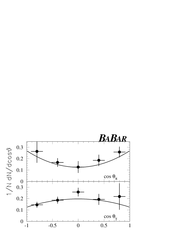
Figure 8: Projections of the number of background-subtracted data events on the $\cos\theta_{\gamma}$ and $\cos\theta_{\pi}$ axes. The result of the two-dimensional fit is overlaid.

5.4 Systematic Errors

Table 2: Sources of systematic error (%) for $B^{0}\rightarrow{D_{s}^{(*)+}D^{*-}}$ branching fractions and $B^{0}\rightarrow{D_{s}^{*+}D^{*-}}$ polarization.

Source	$B^{0}\rightarrow{D_{s}^{+}D^{*-}}$	$B^{0}\rightarrow{D_{s}^{*+}D^{*-}}$	$\sigma(\Gamma_{L}/\Gamma)$
Background subtraction	2.7	5.9	0.5
Monte Carlo statistics	4.2	6.0	2.7
Polarization uncertainty	0.8	0.5	-
Cross Feed	3.2	2.4	-
N${}_{B\overline{B}}$	1.6	1.6	-
${\cal B}(\phi\rightarrow{K^{+}K^{-}})$	1.6	1.6	-
Particle identification	1.0	1.0	0.1
Tracking efficiency	3.6	3.6	0.5
Soft pion efficiency	2.0	2.0	0.2
Relative branching fractions	10.2	10.2	-
${\cal B}({{D_{s}^{*+}}\rightarrow{D_{s}^{+}}\gamma})$	-	2.7	-
Photon efficiency	-	1.3	0.1
$\pi^{0}$ veto	-	2.7	0.3
Total systematic error	13.1	15.1	2.8

The various contributions to the systematic errors of the branching fractions and polarization measurement are summarized in Table 2. The dominant systematic error is due to the uncertainty in our knowledge of the three $D^{+}_{s}$ decay branching fractions. To evaluate the uncertainty due to the background subtraction, the signal yield is determined in an alternative way, by counting the number of events in the histogram after a bin-by-bin subtraction of the background, determined from the Monte Carlo simulation. The difference of the signal yields obtained in this way from the results of section 5 is taken as a systematic error. This also accounts for the systematic error due to a possible deviation of the signal shape from a Gaussian.

The Monte Carlo statistical errors in the determination of the signal and the cross feed efficiencies are propagated to the systematic error. The uncertainty in the calculation of the $B^{0}\rightarrow{D_{s}^{*+}D^{*-}}$ polarization is propagated to the branching fraction systematic error. The systematic error due to charged particle reconstruction efficiency error is 1.2% times the number of charged particles in the decay. An additional error of 1.6% is added in quadrature to account for the uncertainty in the reconstruction efficiency of the soft pion.

The systematic error due to the excluding $\pi^{0}$ overlap ($\pi^{0}$ veto) requirement was studied by measuring the relative yield of inclusive $D_{s}^{*+}$ production in data and Monte Carlo events. To evaluate this error, the selection with and without the $\pi^{0}$ veto was applied for the final photon from ${D_{s}^{*+}}\rightarrow{D_{s}^{+}}\gamma$ decay.

For the polarization measurement, the level of the various backgrounds depends on the charged, neutral and particle identification efficiencies. The fit was repeated varying the background according to the errors in these efficiencies, and the resulting variations in $\Gamma_{L}/\Gamma$ were taken as the associated systematic error.

To check that the simulation accurately reproduces the background $M_{\rm miss}$ distributions in the data, a systematic data-Monte Carlo comparison is made in control samples containing no signal events. These samples are events with $1.78<M_{\rm miss}<1.85$${\mathrm{\,Ge\kern-1.00006ptV\!/}c^{2}}$; events in the $D_{s}^{+}$ sideband $1.89<M_{D_{s}}<1.95$${\mathrm{\,Ge\kern-1.00006ptV\!/}c^{2}}$ or $1.985<M_{D_{s}}<2.05$${\mathrm{\,Ge\kern-1.00006ptV\!/}c^{2}}$; events in the $D_{s}^{*+}$ sideband $170<\Delta M<300$${\mathrm{\,Me\kern-1.00006ptV\!/}c^{2}}$; wrong sign ${{D_{s}^{(*)+}}\pi^{+}}$ combinations in either the $M_{D_{s}}$ and $\Delta M$ sidebands or signal regions (see section 4.1); and candidates in which $M_{\rm miss}$ was calculated using the negative of the CM $D_{s}^{(*)+}$ momentum $p_{{D_{s}^{(*)+}}}^{*}$. The comparison between the data and the Monte Carlo simulation of these control samples is shown in Table 3. The discrepancies indicated in Table 3 are taken into account in the calculation of the systematic errors.

Table 3: The average value $\langle(N_{\rm D}-N_{\rm MC})/N_{\rm MC}\rangle$, averaged over all bins, where $N_{\rm D}$ ($N_{\rm MC}$) is the number of data (Monte Carlo) events in a given bin of the $M_{\rm miss}$ distribution of the given control sample. SB (SR) refers to the $M_{D_{s}}$ or $\Delta M$ sideband (signal region) control sample. WS indicates wrong sign ${{D_{s}^{(*)+}}\pi^{+}}$ combinations, and $-p_{{D_{s}^{(*)+}}}^{*}$ indicates that $M_{\rm miss}$ was calculated using the negative of the $D_{s}^{(*)+}$ CM momentum. The range of the missing mass $1.78<M_{\rm miss}<1.87$${\mathrm{\,Ge\kern-1.00006ptV\!/}c^{2}}$ of the control sample is used except for the first line.

Sample type	${{D_{s}^{+}}\pi^{-}}$	${{D_{s}^{*+}}\pi^{-}}$
$1.78<M_{\rm miss}<1.85$${\mathrm{\,Ge\kern-1.00006ptV\!/}c^{2}}$	$-0.009\pm 0.007$	$\phantom{-}0.075\pm 0.014$
SB	$-0.075\pm 0.006$	$\phantom{-}0.007\pm 0.022$
SR, WS	$\phantom{-}0.006\pm 0.008$	$\phantom{-}0.044\pm 0.015$
SB, WS	$-0.060\pm 0.007$	$-0.008\pm 0.024$
SR, $-p_{{D_{s}^{(*)+}}}^{*}$	$\phantom{-}0.015\pm 0.009$	$\phantom{-}0.075\pm 0.016$
SB, $-p_{{D_{s}^{(*)+}}}^{*}$	$-0.062\pm 0.007$	$-0.123\pm 0.022$
Average	$-0.038\pm 0.003$	$\phantom{-}0.032\pm 0.007$

6 Summary

In summary, using the partial reconstruction technique, we have measured the branching fractions

$${\cal B}(B^{0}\rightarrow{D_{s}^{+}D^{*-}})=(1.03\pm 0.14~{}\mathrm{(stat)}\pm 0.13~{}\mathrm{(syst)}\pm 0.26~{}(\mathrm{syst}~{}{\cal B}({D^{+}_{s}\rightarrow\phi\pi^{+}})))\%$$

and

$${\cal B}(B^{0}\rightarrow{D_{s}^{*+}D^{*-}})=(1.97\pm 0.15~{}\mathrm{(stat)}\pm 0.30~{}\mathrm{(syst)}\pm 0.49~{}(\mathrm{syst}~{}{\cal B}({D^{+}_{s}\rightarrow\phi\pi^{+}})))\%.$$

The fraction of the longitudinal $D_{s}^{*+}$ polarization in $B^{0}\rightarrow{D_{s}^{*+}D^{*-}}$ is determined to be

$$\Gamma_{L}/\Gamma=(51.9\pm 5.0~{}\mathrm{(stat)}\pm 2.8~{}\mathrm{(syst)})\%.$$

This measurement is consistent with the theoretical prediction of (53.5$\pm$3.3)% [9] assuming factorization. Our preliminary results are also in a good agreement with previous experimental results [3, 10].

7 Acknowledgments

We are grateful for the extraordinary contributions of our PEP-II colleagues in achieving the excellent luminosity and machine conditions that have made this work possible. The success of this project also relies critically on the expertise and dedication of the computing organizations that support BABAR. The collaborating institutions wish to thank SLAC for its support and the kind hospitality extended to them. This work is supported by the US Department of Energy and National Science Foundation, the Natural Sciences and Engineering Research Council (Canada), Institute of High Energy Physics (China), the Commissariat à l’Energie Atomique and Institut National de Physique Nucléaire et de Physique des Particules (France), the Bundesministerium für Bildung und Forschung and Deutsche Forschungsgemeinschaft (Germany), the Istituto Nazionale di Fisica Nucleare (Italy), the Research Council of Norway, the Ministry of Science and Technology of the Russian Federation, and the Particle Physics and Astronomy Research Council (United Kingdom). Individuals have received support from the A. P. Sloan Foundation, the Research Corporation, and the Alexander von Humboldt Foundation.

References

- [1] CLEO Collaboration, G. Bonvicini et al., CLEO CONF 98-23, presented at the 29th International Conference on High Energy Physics, Vancouver, Canada (1998).
- [2] CLEO Collaboration, D. Cinabro et al., hep-ex/0009045, presented at the 30th International Conference on High Energy Physics, Osaka, Japan (2000).
- [3] CLEO Collaboration, S. Ahmed et al., Phys. Rev. D 62, 112003 (2000).
- [4] BABAR Collaboration, A. Palano et al., Nucl. Instrum. Methods. A479, 1 (2002).
- [5] G. C. Fox and S. Wolfram, Phys. Rev. Lett. 41, 1581 (1978); G. C. Fox and S. Wolfram, Nucl. Phys. B 149 413 (1979).
- [6] Particle Data Group, K. Hagiwara et al., Phys. Rev. D 66, 010001 (2002).
-
[7]