New Measurements of the $D^{+}\rightarrow\overline{K}^{*0}\mu^{+}\nu$ Form Factor Ratios

Abstract

Using a large sample of $D^{+}\rightarrow K^{-}\pi^{+}\mu^{+}\nu$ decays collected by the FOCUS photoproduction experiment at Fermilab, we present new measurements of two semileptonic form factor ratios: $r_{v}$ and $r_{2}$. We find $r_{v}=1.504\pm 0.057\pm 0.039{}$ and $r_{2}=0.875\pm 0.049\pm 0.064{}$. Our form factor results include the effects of the $s$-wave interference discussed in Reference [1].

The FOCUS Collaboration

1 Introduction

This paper provides new measurements of the parameters that describe $D^{+}\rightarrow K^{-}\pi^{+}\mu^{+}\nu$ decay. In an earlier paper [1] we described this process as the interference of a $D^{+}\rightarrow\overline{K}^{*0}\mu^{+}\nu$ amplitude with a constant $s$-wave amplitude. The $D^{+}\rightarrow\overline{K}^{*0}\mu^{+}\nu$ decay amplitude is described [2] by four form factors with an assumed (pole form) $q^{2}$ dependence. Following earlier experimental work  [3, 4, 5, 6, 7, 8], the $D^{+}\rightarrow\overline{K}^{*0}\mu^{+}\nu$ amplitude is then described by ratios of form factors taken at $q^{2}$ = 0. The traditional set is: $r_{2}$, $r_{3}$, and $r_{v}$ which we define explicitly after Equation 8.

Five kinematic variables that uniquely describe $D^{+}\rightarrow K^{-}\pi^{+}\mu^{+}\nu$ decay are illustrated in Figure 1. These are the $K^{-}\pi^{+}$ invariant mass ($m_{K\pi}$) , the square of the $\mu\nu$ mass ($q^{2}$), and three decay angles: the angle between the $\pi$ and the $D$ direction in the $K^{-}\pi^{+}$ rest frame ($\theta_{\textrm{v}}$), the angle between the $\nu$ and the $D$ direction in the $\mu\nu$ rest frame ($\theta_{\ell}$), and the acoplanarity angle between the two decay planes ($\chi$). These angular conventions on $\theta_{\ell}$ and $\theta_{\textrm{v}}$ apply to both the $D^{+}$ and $D^{-}$. The sense of the acoplanarity variable is defined via a cross product expression of the form: $(\vec{P}_{\mu}\times\vec{P}_{\nu})\times(\vec{P}_{K}\times\vec{P}_{\pi})\cdot\vec{P}_{K\pi}$ where all momentum vectors are in the $D^{+}$ rest frame. Since this expression involves five momentum vectors, as one goes from $D^{+}\rightarrow D^{-}$ one must change $\chi\rightarrow-\chi$ in Equation 8 to get the same intensity for the $D^{+}$ and $D^{-}$ assuming CP symmetry.

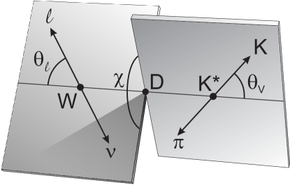
Figure 1: Definition of kinematic variables.

Using the notation of [2], we write the decay distribution for $D^{+}\rightarrow K^{-}\pi^{+}\mu^{+}\nu$ in terms of the four helicity basis form factors: $H_{+}~{},~{}H_{0}~{},~{}H_{-}~{},H_{t}$.

$${d^{5}\Gamma\over dm_{K\pi}~{}dq^{2}~{}d\cos\theta_{\textrm{v}}~{}d\cos\theta_{\ell}~{}d\chi}\propto K(q^{2}{}-m_{l}^{2})\left\{\left|\begin{array}[]{l}(1+\cos\theta_{\ell})\sin\theta_{\textrm{v}}e^{i\chi}\textrm{B}_{K^{*0}}H_{+}\\ -\,(1-\cos\theta_{\ell})\sin\theta_{\textrm{v}}e^{-i\chi}\textrm{B}_{K^{*0}}H_{-}\\ -\,2\sin\theta_{\ell}(\cos\theta_{\textrm{v}}\textrm{B}_{K^{*0}}+Ae^{i\delta})H_{0}\\ \end{array}\right|^{2}\right.$$ (4)

$$+\frac{m^{2}_{\ell}}{q^{2}}\left.\left|\begin{array}[]{l}\sin\theta_{\ell}\sin\theta_{\textrm{v}}\textrm{B}_{K^{*0}}\left(e^{i\chi}H_{+}+e^{-i\chi}H_{-}\right)\\ +\,2\cos\theta_{\ell}\left(\cos\theta_{\textrm{v}}\textrm{B}_{K^{*0}}+Ae^{i\delta}\right)H_{0}\\ +\,2\left(cos\theta_{\textrm{v}}\textrm{B}_{K^{*0}}+Ae^{i\delta}\right)H_{t}\end{array}\right|^{2}\right\}\phantom{xxx}$$ (8)

where $K$ is the momentum of the $K^{-}\pi^{+}$ system in the rest frame of the $D^{+}$. The first term gives the intensity for the $\mu^{+}$ to be right-handed, while the (highly suppressed) second term gives the intensity for it to be left-handed. The helicity basis form factors are given by:

$$H_{\pm}(q^{2}) = (M_{D}+m_{K\pi})A_{1}(q^{2})\mp 2{M_{D}K\over M_{D}+m_{K\pi}}V(q^{2})$$

$$H_{0}(q^{2}) = {1\over 2m_{K\pi}\sqrt{q^{2}}}\left[(M^{2}_{D}-m^{2}_{K\pi}-q^{2})(M_{D}+m_{K\pi})A_{1}(q^{2})-4{M^{2}_{D}K^{2}\over M_{D}+m_{K\pi}}A_{2}(q^{2})\right]$$

$$H_{t}(q^{2}) = {M_{D}K\over M_{K\pi}\sqrt{q^{2}}}\left[(M_{D}+M_{K\pi})A_{1}(q^{2})-{(M^{2}_{D}-M^{2}_{K\pi}+q^{2})\over M_{D}+M_{K\pi}}A_{2}(q^{2})+{2q^{2}\over M_{D}+M_{K\pi}}A_{3}(q^{2})\right]$$

The vector and axial form factors are generally parameterized by a pole dominance form:

$$A_{i}(q^{2})={A_{i}(0)\over 1-q^{2}/M_{A}^{2}}~{}~{}~{}~{}~{}~{}~{}~{}V(q^{2})={V(0)\over 1-q^{2}/M_{V}^{2}}$$

where we use nominal (spectroscopic) pole masses of $M_{A}=2.5~{}\textrm{GeV}/c^{2}$ and $M_{V}=2.1~{}\textrm{GeV}/c^{2}$.

The $\textrm{B}_{K^{*0}}$ denotes the Breit-Wigner amplitude describing the $\overline{K}^{*0}$ resonance:

$$\textrm{B}_{K^{*0}}=\frac{\sqrt{m_{0}\Gamma\,}\left(\frac{P^{*}}{P_{0}^{*}}\right)}{m_{K\pi}^{2}-m_{0}^{2}+im_{0}\Gamma\left(\frac{P^{*}}{P_{0}^{*}}\right)^{3}}$$

Under these assumptions, the decay intensity is then parameterized by the $r_{v}{}\equiv V(0)/A_{1}(0)~{},~{}r_{2}{}\equiv A_{2}(0)/A_{1}(0)~{},~{}r_{3}{}\equiv A_{3}(0)/A_{1}(0)$ form factor ratios describing the $D^{+}\rightarrow\overline{K}^{*0}\mu^{+}\nu$ amplitude and the modulus $A$ and phase $\delta$ describing the $s$-wave amplitude. Throughout this paper, unless explicitly stated otherwise, the charge conjugate is also implied when a decay mode of a specific charge is stated.

2 Experimental and analysis details

The data for this paper were collected in the Wideband photoproduction experiment FOCUS during the Fermilab 1996–1997 fixed-target run. In FOCUS, a forward multi-particle spectrometer is used to measure the interactions of high energy photons on a segmented BeO target. The FOCUS detector is a large aperture, fixed-target spectrometer with excellent vertexing and particle identification. Most of the FOCUS experiment and analysis techniques have been described previously [1, 9, 10, 11]. Our analysis cuts were chosen to give reasonably uniform acceptance over the five kinematic decay variables, while maintaining a strong rejection of backgrounds. To suppress background from the re-interaction of particles in the target region which can mimic a decay vertex, we required that the charm secondary vertex was located at least one standard deviation outside of all solid material including our target and target microstrip system.

To isolate the $D^{+}\rightarrow K^{-}\pi^{+}\mu^{+}\nu$ topology, we required that candidate muon, pion, and kaon tracks appeared in a secondary vertex with a confidence level exceeding 5%. The muon track, when extrapolated to the shielded muon arrays, was required to match muon hits with a confidence level exceeding 5%. The kaon was required to have a Čerenkov light pattern more consistent with that for a kaon than that for a pion by 1 unit of log likelihood, while the pion track was required to have a light pattern favoring the pion hypothesis over that for the kaon by 1 unit [11].

To further reduce muon misidentification, a muon candidate was allowed to have at most one missing hit in the 6 planes comprising our inner muon system and an energy exceeding 10 GeV. In order to suppress muons from pions and kaons decaying within our apparatus, we required that each muon candidate had a confidence level exceeding 2% to the hypothesis that it had a consistent trajectory through our two analysis magnets.

Non-charm and random combinatoric backgrounds were reduced by requiring both a detachment between the vertex containing the $K^{-}\pi^{+}\mu^{+}$ and the primary production vertex of 10 standard deviations and a minimum visible energy $(E_{K}+E_{\pi}+E_{\mu})$ of 30 GeV. To suppress possible backgrounds from higher multiplicity charm decay, we isolate the $K\pi\mu$ vertex from other tracks in the event (not including tracks in the primary vertex) by requiring that the maximum confidence level for another track to form a vertex with the candidate be less than 0.1%.

In order to allow for the missing energy of the neutrino in this semileptonic $D^{+}$ decay, we required the reconstructed $K\pi\mu$ mass be less than the nominal $D^{+}$ mass. Background from $D^{+}\rightarrow K^{-}\pi^{+}\pi^{+}$, where a pion is misidentified as a muon, was reduced using a mass cut: we required when the muon track is treated as a pion and the combination is reconstructed as a $K\pi\pi$, the $K\pi\pi$ invariant mass differed from the nominal $D^{+}$ mass by at least three standard deviations. In order to suppress background from $D^{*+}\rightarrow D^{0}\pi^{+}\rightarrow(K^{-}\mu^{+}\nu)\pi^{+}$ we required $M(K^{-}\mu^{+}\nu\pi^{+})-M(K^{-}\mu^{+}\nu)>0.18~{}\textrm{GeV}/c^{2}$. The $m_{K\pi}$ distribution for our $D^{+}\rightarrow K^{-}\pi^{+}\mu^{+}\nu$ candidates is shown in Figure 2.

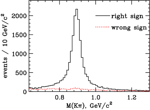
Figure 2: $D^{+}\rightarrow K^{-}\pi^{+}\mu^{+}\nu$ signal. Right-sign and wrong-sign samples are shown. In the mass window from 0.8–1.0 $\textrm{GeV}/c^{2}$ there is a right-sign excess of 14 678 events. A Monte Carlo that simulates the production and decay of all known charm species predicts that $\approx$3% of this excess is actually background from other charm decays.

The technique used to reconstruct the neutrino momentum through the $D^{+}$ line-of-flight, and tests of our ability to simulate the resolution on kinematic variables that rely on the neutrino momentum are described in Reference [1].

3 Fitting Technique

We use a binned version [12] of the fitting technique developed by the E691 Collaboration [13] for fitting decay intensities where some of the kinematic variables have very poor resolution such as the four variables that rely on reconstructed neutrino kinematics. The observed number of wrong-sign-subtracted events in each kinematic bin is compared to a prediction. The production is constructed from a $D^{+}\rightarrow K^{-}\pi^{+}\mu^{+}\nu$ signal Monte Carlo incorporating $s$-wave interference  [1] plus a wrong-sign-subtracted, charm background contribution predicted by a background Monte Carlo which simulates all known charm decays as well as our misidentification levels.

Although the charm background correction was fairly unimportant given the tight muon cuts used for our quoted results, this correction was important when looser muon cuts were employed. In the sample selected with looser muon cuts, the charm background increased from about 3% to 7% of the total right-sign excess. In fits to the looser sample, the charm background correction typically lowered the uncorrected $r_{v}$ by 0.15 (or about 2.7 times our statistical error) to a value very consistent with our quoted result. The charm background is primarily due to false muons from decays of pions and kaons in flight and therefore tends to populate low (lab) momentum or the negative $\cos\theta_{\ell}$ region. Including the background correction to the fit reduced the apparent backward-forward asymmetry in $\cos\theta_{\ell}$, thus reducing the difference between the $H_{+}$ and $H_{-}$ form factor in Equation 8. Since this difference is proportional to $r_{v}$, fits with the background correction will have a lower $r_{v}$ relative to fits where no charm background correction was performed. The effect of charm backgrounds on the $r_{2}$ form factor ratio was found to be much smaller — about $1\sigma$ for our “loose” muon fits.

The signal Monte Carlo was initially generated flat in the $K\pi\mu\nu$ phase space and the five generated as well as reconstructed kinematic variables were stored for each event. The signal prediction for a given fit iteration is then computed by weighting each event within a given reconstructed kinematic bin by the intensity given by Equation 8 evaluated using the five generated kinematic variables for the current set of fit parameters. The background Monte Carlo was normalized to the observed number of $D^{+}\rightarrow K^{-}\pi^{+}\mu^{+}\nu$ events in the mass range $0.8<m_{K\pi}<1.0~{}\textrm{GeV}/c^{2}{}$ after applying the wrong-sign subtraction. The signal Monte Carlo was normalized to the difference between the observed wrong-sign-subtracted yield and the predicted wrong-sign-subtracted background yield. The fit determined the physics parameters by minimizing the $\chi^{2}$ over all bins.

Two fits were employed in this analysis: a fit to the $s$-wave amplitude with fixed $r_{v}$ and $r_{2}$ form factor ratios, and a fit to the $r_{v}$ and $r_{2}$ form factors ratios with a fixed $s$-wave amplitude and phase. In the form factor fit, we used five bins in $\cos\theta_{\textrm{v}}$, five bins in $\cos\theta_{\ell}$, three bins in $|\chi|$, and three bins in $q^{2}{}/q^{2}_{\rm max}$ for a total of 225 bins. This binning was chosen to be sensitive to the main features of our model intensity, Equation 8, that depend on $r_{v}$ and $r_{2}$. The $s$-wave amplitude used three bins of $\cos\theta_{\textrm{v}}$ , three bins of $\cos\theta_{\ell}$, four bins of $m_{K\pi}$, and three bins of $\chi$ for a total of 108 bins. The $s$-wave amplitude binning was chosen to emphasize the $m_{K\pi}$ dependence of the angular distribution. This dependence is extremely sensitive to the $s$-wave phase as discussed in Reference [1]. In both cases, evenly spaced bins were used. The binnings of both fits were chosen to ensure at least 10 observed events per fit bin. These two fits were very loosely coupled so only a few iterations sufficed to obtain stable results.

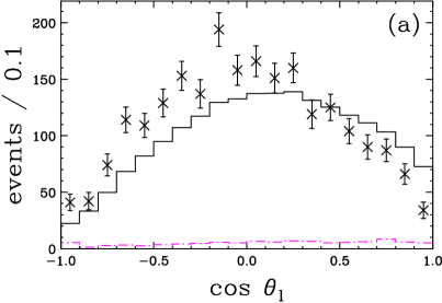
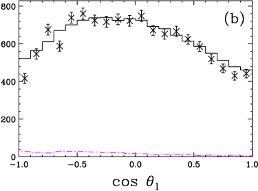
Figure 3: We show the $\cos\theta_{\ell}$ distribution in two ranges for $q^{2}$. The data are shown as points with error bars, while the Monte Carlo model which includes charm backgrounds are the solid line histograms. The predicted charm background contributions are the dashed lines. Figure (a) shows events in the low $q^{2}$ region : $q^{2}{}<0.2~{}\textrm{GeV}^{2}/c^{2}{}$. Figure (b) shows events in the remaining $q^{2}$ region : $q^{2}{}>0.2~{}\textrm{GeV}^{2}/c^{2}{}$.

Our initial form factor fits were of very poor quality due to a problem with our model matching the $\cos\theta_{\ell}$ distribution at very low $q^{2}$ ($q^{2}{}<0.2~{}\textrm{GeV}^{2}/c^{2}{}$). Figure 3 illustrates this problem by comparing the $\cos\theta_{\ell}$ distribution in data and our model for events below $q^{2}$ = 0.2 $\textrm{GeV}^{2}/c^{2}$ and above $q^{2}$ = 0.2 $\textrm{GeV}^{2}/c^{2}$ where the discrepancy is far less. Excluding the $q^{2}{}<0.2~{}\textrm{GeV}^{2}/c^{2}{}$ region caused the $\chi^{2}$ of our fits to reduce by 86 units. The low $q^{2}$ discrepancy can most easily be explained as a deviation from the assumed pole dominance of the vector form factor, $V(q^{2}{})$, but we have not eliminated all other possibilities. We have decided to exclude this region from our form factor and $s$-wave amplitude fits. When these regions were excluded, the fitted $r_{v}$ and $r_{2}$ form factor ratios decreased by 1.2 $\sigma$ and 0.4 $\sigma$ respectively. With the $q^{2}{}<0.2~{}\textrm{GeV}^{2}/c^{2}{}$ removed, our form factor fit has a $\chi^{2}$ per degree of freedom of 1.15 for 223 degrees of freedom or a confidence level of 5.2%.

Figures 4 and 5 compare the data and model for several of the more interesting projections of $\cos\theta_{\textrm{v}}$, $\cos\theta_{\ell}$, $\chi$ and $q^{2}$. No $q^{2}$ cut is applied in these projections. Most of these distributions follow the predicted values reasonably well with the exception of the low $q^{2}{}$ $\cos\theta_{\ell}$ projection (Figure 4 (c)) for the reasons discussed above.

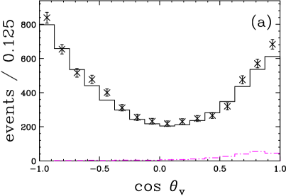
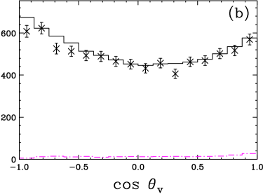
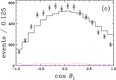
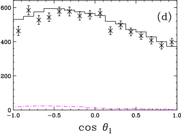
Figure 4: Various $\cos\theta_{\textrm{v}}$ and $\cos\theta_{\ell}$ projections. The data are the points with error bars. The MC model predictions are the solid line histograms. The predicted charm background projections are the dashed lines. The model distributions are normalized by the total number of events in the sample rather than the area of each individual plot. (a) The $\cos\theta_{\textrm{v}}$ distribution for $q^{2}$/$q^{2}{}_{\rm max}<0.5$ (b) The $\cos\theta_{\textrm{v}}$ distribution for $q^{2}$/$q^{2}{}_{\rm max}>0.5$ (c) The $\cos\theta_{\ell}$ distribution for $q^{2}$/$q^{2}{}_{\rm max}<0.5$ (d) The $\cos\theta_{\ell}$ distribution for $q^{2}$/$q^{2}{}_{\rm max}>0.5$

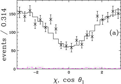
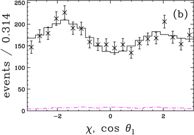
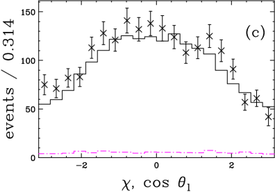
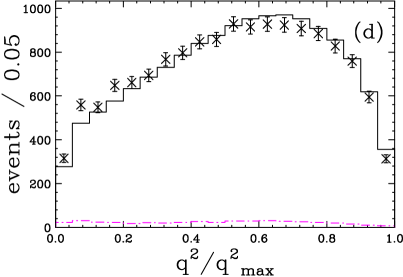
Figure 5: Acoplanarity projections with $\cos\theta_{\ell}{}<0$ and three ranges of $\cos\theta_{\textrm{v}}$. (a) $\cos\theta_{\textrm{v}}{}<-0.5$ (b) $-0.5<\cos\theta_{\textrm{v}}{}<0.5$ and (c) $0.5<\cos\theta_{\textrm{v}}{}$. (d) The $q^{2}/q^{2}_{\rm max}$ projection. The data are the points with error bars. The models are the solid line histograms. The predicted charm backgrounds are the dashed lines.

The expected relative amounts of the $\cos{\chi}$ and $\cos{2\chi}$ contributions and their phase variation as a function of $\cos\theta_{\textrm{v}}$ is well reproduced by our data as is the $\chi\leftrightarrow-\chi$ asymmetry created by the $s$-wave interference. The respective $\cos\theta_{\ell}{}>0$ projections in data are also well matched by the model but show less variation than the acoplanarity distributions shown in Figure 5.

Our $s$-wave amplitude fit produced an amplitude modulus of $A=0.330\pm 0.022\pm 0.015~{}\rm{GeV}^{-1}$ and a phase of $\delta=0.68\pm 0.07\pm 0.05~{}{\rm rad}$. Our estimate of the $s$-wave systematic error was based on the sample variance over 35 fits run with different analysis cuts. We varied such cuts as the particle identification cuts, vertexing cuts, and visible mass and energy cuts.

This result was then fed into our form factor fit to produce our $r_{v}$ and $r_{2}$ measurements values.

A far more extensive systematic error analysis was made for the form factor analysis since these are actual physical parameters rather than an effective description of an interfering amplitude which is only validated in the vicinity of the $\overline{K}^{*0}$ pole.

4 Form Factor Ratio Systematic Errors

Three basic approaches were used to determine the systematic error on the form factor ratios. In the first approach, we measured the stability of the branching ratio with respect to variations in analysis cuts designed to suppress backgrounds. In these studies we varied cuts such as the detachment criteria, the secondary vertex quality, the minimal number of tracks in our primary vertex, particle identification cuts, visible momenta cuts, etc. Fifteen such cut sets were considered. In the second approach, we split our sample according to a variety of criteria deemed relevant to our acceptance, production, and decay models and estimated a systematic based on the consistency of the form factor ratio measurements among the split samples. We split our sample based on the visible $D^{+}$ momentum, particle versus antiparticle, and whether or not the $m_{K\pi}$ mass was above or below 0.9 $\textrm{GeV}/c^{2}$. This later split was based on our previous observation [1] of a large $\cos\theta_{\textrm{v}}$ asymmetry that developed for events with $m_{K\pi}{}<0.9~{}\textrm{GeV}/c^{2}{}$ due to the $s$-wave amplitude interference. In the third approach we checked the stability of the branching fraction as we varied specific parameters in our Monte Carlo model and fitting procedure. These included varying the level of the charm background Monte Carlo, and the value of the $r_{3}$ form factor ratio as a uniform variable over the range $-2<r_{3}<2$.

Leaving out the $s$-wave amplitude contribution in our form factor fits entirely shifted both $r_{v}$ and $r_{2}$ downward by only $0.5\sigma$. Given the insensitivity of our form factor fits to the $s$-wave amplitude, no systematic error was assessed for uncertainty in the $s$-wave parameters. Combining all three non-zero systematic error estimates in quadrature we find $r_{v}=1.504\pm 0.057\pm 0.039{}$ and $r_{2}=0.875\pm 0.049\pm 0.064{}$.

5 Summary

We presented a fit of the $s$-wave amplitude. We obtained an amplitude modulus of $A=0.330\pm 0.022\pm 0.015~{}{\rm GeV}^{-1}$ and a phase of $\delta=0.68\pm 0.07\pm 0.05~{}{\rm rad}$ in reasonable agreement with our very informal, previous [1] estimate of $A=0.36\exp(i\pi/4)~{}{\rm GeV}^{-1}$. The inclusion of the $s$-wave amplitude dramatically improved the the quality of our form factor fits but created only minor shifts in the resulting form factor ratio values.

Table 1: Measurements of the $D^{+}\rightarrow\overline{K}^{*0}\ell^{+}\nu_{\ell}$ form factor ratios

Group	$r_{v}$	$r_{2}$
This work	$1.504\pm 0.057\pm 0.039$	$0.875\pm 0.049\pm 0.064$
BEATRICE [3]	$1.45\pm 0.23\pm 0.07$	$1.00\pm 0.15\pm 0.03$
E791 (e) [4]	$1.90\pm 0.11\pm 0.09$	$0.71\pm 0.08\pm 0.09$
E791 ($\mu$) [5]	$1.84\pm 0.11\pm 0.09$	$0.75\pm 0.08\pm 0.09$
E687 [6]	$1.74\pm 0.27\pm 0.28$	$0.78\pm 0.18\pm 0.11$
E653 [7]	$2.00\pm 0.33\pm 0.16$	$0.82\pm 0.22\pm 0.11$
E691 [8]	$2.0\pm 0.6\pm 0.3$	$0.0\pm 0.5\pm 0.2$

Table 1 summarizes measurements of the $r_{v}$ and $r_{2}$ form factor ratios. Our measurement is the first one to include the effects on the acceptance due to changes in the decay angular distribution brought about by the $s$-wave interference. We are consistent with the most recent previous measurement by the BEATRICE Collaboration. Our $r_{v}$ value is about 2.9 standard deviations below the average of the two (previously most precise) measurements by the E791 Collaboration although consistent with their value of $r_{2}$.

6 Acknowlegments

We wish to acknowledge the assistance of the staffs of Fermi National Accelerator Laboratory, the INFN of Italy, and the physics departments of the collaborating institutions. This research was supported in part by the U. S. National Science Foundation, the U. S. Department of Energy, the Italian Istituto Nazionale di Fisica Nucleare and Ministero dell’Università e della Ricerca Scientifica e Tecnologica, the Brazilian Conselho Nacional de Desenvolvimento Científico e Tecnológico, CONACyT-México, the Korean Ministry of Education, and the Korean Science and Engineering Foundation.

References

• [1] FOCUS Collab., J.M. Link et al., Phys. Lett. B 535 (2002) 43.
• [2] J.G. Korner and G.A. Schuler, Z. Phys. C 46 (1990) 93.
• [3] BEATRICE Collab., M. Adamovich et al., Eur. Phys. J. C 6 (1999) 35.
• [4] E791 Collab., E. M. Aitala et al., Phys. Rev. Lett. 80 (1998) 1393.
• [5] E791 Collab., E. M. Aitala et al., Phys. Lett. B 440 (1998) 435.
• [6] E687 Collab., P.L. Frabetti et al., Phys. Lett. B 307 (1993) 262.
• [7] E653 Collab., K. Kodama et al., Phys. Lett. B 274 (1992) 246.
• [8] E691 Collab., J. C. Anjos et al., Phys. Rev. Lett. 65 (1990) 2630.
• [9] E687 Collab., P. L. Frabetti et al., Nucl. Instrum. Methods A 320 (1992) 519.
• [10] FOCUS Collab., J. M. Link et al., Phys. Lett. B 485 (2000) 62.
• [11] FOCUS Collab., J. M. Link et al., Nucl. Instrum. Methods A 484 (2002) 270.
• [12] E687 Collab., P. L. Frabetti et al., Phys. Lett. B 364 (1995) 127.
• [13] D.M. Schmidt, R.J. Morrision, and M.S. Witherell, Nucl. Instrum. Methods. A 328 (1993) 547.