A Search for Time-Dependent $B_{s}^{0}-\overline{B_{s}^{0}}$ Oscillations
Using Exclusively Reconstructed $D^{\pm}_{s}$ Mesons

Abstract

A search for $B_{s}^{0}-\overline{B_{s}^{0}}$ oscillations is performed using a sample of 400,000 hadronic $Z^{0}$ decays collected by the SLD experiment. The $B_{s}^{0}$ candidates are reconstructed in the $B_{s}^{0}\rightarrow D_{s}^{-}X$ channel with $D_{s}^{-}\rightarrow\phi\pi^{-}$, $K^{*0}K^{-}$. The $B_{s}^{0}$ production flavor is determined using the large forward-backward asymmetry of polarized $Z^{0}\rightarrow b\overline{b}$ decays and charge information in the hemisphere opposite that of the $B_{s}^{0}$ candidate. The decay flavor is tagged by the charge of the $D_{s}^{\pm}$. From a sample of 361 candidates with an average $B_{s}^{0}$ purity of 40%, we exclude the following values of the oscillation frequency: $\Delta m_{s}<1.4$ ps^-1 and $2.4<\Delta m_{s}<5.3$ ps^-1 at the 95% confidence level.

I Introduction

The primary motivation for studying neutral $B$ meson oscillations is to measure the poorly known Cabibbo-Kobayashi-Maskawa (CKM) matrix element $V_{td}$. The $B_{d}^{0}$ oscillation frequency corresponds to the mass difference, $\Delta m_{d}$, between the physical eigenstates of the $B_{d}^{0}-\overline{B_{d}^{0}}$ system, which is sensitive to $|V_{td}|$. Although $\Delta m_{d}$ is measured to within 2.5% PDG2001 , theoretical uncertainties lead to a 20% uncertainty in the extraction of $|V_{td}|$ Bernard:2000ki . However, many uncertainties cancel in the ratio of mass differences in the $B_{d}^{0}$ and $B_{s}^{0}$ systems:

$${\Delta m_{s}\over\Delta m_{d}}={m_{B_{s}}f_{B_{s}}^{2}B_{B_{s}}\over m_{B_{d}}f_{B_{d}}^{2}B_{B_{d}}}\left|{V_{ts}\over V_{td}}\right|^{2}=(1.15\pm 0.05)^{2}\left|{V_{ts}\over V_{td}}\right|^{2},$$ (1)

where $m_{B_{d}}$ and $m_{B_{s}}$ are the $B$ meson masses, $f_{B_{d}}$ and $f_{B_{s}}$ are the decay constants, and $B_{B_{d}}$ and $B_{B_{s}}$ are the “B-parameters”. Using this formula, and assuming $|V_{ts}|$=$|V_{cb}|$, one can obtain a 5-10% theoretical uncertainty on $|V_{td}|$ Bernard:2000ki ; Kronfeld:2002ab .

As yet, the $B_{s}^{0}$ oscillation frequency has not been measured. The published lower limit on $\Delta m_{s}$ based on the combined results from ALEPH, DELPHI, OPAL and CDF is 13.1 ps^-1 at the 95% confidence level PDG2001 . In the context of the Standard Model, other measurements suggest that $\Delta m_{s}$ may be just beyond this current limit CIUCHINI .

This letter describes a study cjlthesis of $B_{s}^{0}-\overline{B_{s}^{0}}$ oscillations with the SLD experiment at SLAC. The measurement of $B_{s}^{0}$ mixing requires excellent decay time resolution in order to resolve the very fast oscillations. The technique described in this letter, using $B_{s}^{0}\rightarrow D_{s}^{-}X$ decays conjugate with $D_{s}^{-}\rightarrow\phi\pi^{-}$ or $K^{*0}K^{-}$, has excellent decay length resolution (the best of any $B_{s}^{0}$ analysis to date) and high purity (reconstruction of a $D_{s}^{-}$ helps to discriminate against the prominent backgrounds from $B^{+}$ and $B_{d}^{0}$ mesons). This work also represents the first use of polarized beams in a search for $B_{s}^{0}$ mixing, which provide an effective new means of identifying the flavor of the $B_{s}^{0}$ meson at production.

II Apparatus and Event Selection

This analysis is based on a data set of 400,000 events of the form $e^{+}e^{-}\rightarrow Z^{0}\rightarrow hadrons$, collected from 1996 through 1998 by the SLD experiment. A detailed description of the experiment can be found elsewhere SLDTDR ; sldpaper . The analysis uses charged tracks reconstructed in the Central Drift Chamber (CDC) and the pixel-based CCD vertex detector (VXD3). The momentum resolution from the combined CDC and VXD3 fit is determined to be $\sigma_{p\perp}/p_{\perp}=0.010\oplus 0.0024p_{\perp}$, where $p_{\perp}$ (in GeV/c) is the momentum of the track transverse to the beamline. The track impact parameter resolution in the transverse plane is $\sigma_{xy}=8\oplus 33/(p\sin^{3/2}\theta)$ $\mu m$ and along the beam direction is $\sigma_{z}=10\oplus 33/(p\sin^{3/2}\theta)$ $\mu m$, where $p$ (in GeV/c) is the track momentum and $\theta$ is the polar angle with respect to the electron beam. The tracking system is surrounded by the Cherenkov Ring Imaging Detector (CRID), a two-radiator system that allows good pion and kaon separation in the momentum range between 0.3 and 35 GeV/c.

The goal of the analysis is to measure or constrain the oscillation frequency. This is accomplished by using $B_{s}^{0}$ decay candidates that are flavor tagged at both production and decay, and by measuring the proper time of the decay through measurements of the $B_{s}^{0}$ decay length and energy. The decay time distributions of $B$ mesons whose flavor at production and decay are different (the same), so called mixed (unmixed) events, are modulated by the oscillation frequency. A fit to these distributions constrains $\Delta m_{s}$.

Event reconstruction consists of four main steps: hadronic event selection, $Z^{0}\rightarrow b\overline{b}$ event selection, $D_{s}^{-}$ decay reconstruction, and partial reconstruction of $B_{s}^{0}$ decays. A hadronic event is identified as having at least seven charged tracks, a total energy of at least 18 GeV, and an event thrust axis satisfying $|cos\theta_{thrust}|<0.85$. The thrust axis is calculated based on the energy clusters found in the liquid-argon calorimeter. The hadronic event selection removes essentially all dilepton events and other non-hadronic backgrounds. To enhance the fraction of $Z^{0}\rightarrow b\overline{b}$ events in the sample, events are required to have at least one topologically reconstructed secondary vertex bzvtop with a vertex mass greater than 2 GeV in either hemisphere. The vertex mass calculation includes a correction for the missing momentum transverse to the $B$ flight direction in order to partially account for missing particles. A neural network btom is used to select a candidate secondary $B$ vertex (if multiple topological secondary vertices exist) and its decay tracks. The resulting event sample is 97% pure $b\overline{b}$ with a single hemisphere $b$ tagging efficiency of 54%.

The $D_{s}^{-}$ is reconstructed in one of two modes, $D_{s}^{-}\rightarrow\phi\pi^{-}~{}{\rm or}~{}K^{*0}K^{-}\rightarrow K^{+}K^{-}\pi^{-}$. Oppositely charged tracks are first paired to form a $\phi$ ($K^{*0}$) candidate and a third track is then attached to form a $D_{s}^{-}$ candidate. To maximize the discrimination between true $D_{s}^{-}$ and combinatorial background events, kinematic information for the $D_{s}^{-}$ candidate is fed into another neural network. In this case, the neural net inputs include CRID particle identification information for each of the three daughter tracks, the $K^{+}K^{-}$ ($K^{-}\pi^{+}$) invariant mass for $\phi$ ($K^{*0}$) candidates, the fit probability for the $D_{s}^{-}$ decay vertex, the $D_{s}^{-}$ decay length normalized by the decay length error, the total momentum of the $D_{s}^{-}$, the angle between the neutral meson ($\phi$ or $K^{*0}$) momentum in the $D_{s}^{-}$ rest frame and the $D_{s}^{-}$ flight direction, and the angle between the $\pi^{-}$ or $K^{-}$ from the $D_{s}^{-}$ decay and the $K^{+}$ from the neutral meson decay in the rest frame of the neutral meson. The neural net cut that maximizes the sensitivity of the analysis to $B_{s}^{0}$ mixing is determined separately for each of the two $D_{s}^{-}$ decay modes. The resulting $KK\pi$ mass distribution for both modes combined is shown in Figure 1.

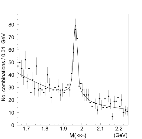
Figure 1: Distribution of $KK\pi$ invariant mass for $\phi\pi$ and $K^{*0}K$ candidates combined, for the events that include a $B_{s}^{0}$ candidate vertex. The solid line shows a fit with the same functional form as is used in the likelihood function: two Gaussian distributions with common mean for the $D_{s}$ signal, a single Gaussian for the $D^{+}$ contribution and a second-order polynomial for the background.

The $B_{s}^{0}$ decay vertex is found by vertexing the virtual $D_{s}^{-}$ track with other tracks in the hemisphere. The virtual $D_{s}^{-}$ track is constructed by combining the 4-momenta of the three daughter tracks and constraining the parent $D_{s}^{-}$ to pass through the decay vertex. The parent track error matrix is determined from propagation of the track measurement errors of the daughters. The $B_{s}^{0}$ vertex fit is accomplished in two steps: 1) identify an intersection of the virtual $D_{s}^{-}$ track with another charged track in the same hemisphere to act as a seed for the $B_{s}^{0}$ decay vertex and 2) add other charged tracks to the seed vertex if they are more consistent with coming from the $B_{s}^{0}$ decay than coming from the primary interaction point (IP). To find the seed, the $D_{s}^{-}$ track is individually vertexed with each track (excluding $D_{s}^{-}$ daughters) in the same hemisphere. The vertex that is farthest from the IP and upstream of the $D_{s}^{-}$ (or consistent with being upstream within 5$\sigma$) and has a vertex fit $\chi^{2}$ of less than 5 is chosen as the seed. In order to determine if another track should be added to the vertex, we examine two parameters: 1) the distance D from the IP to the seed vertex and 2) the distance L along the same direction from the IP to the point of closest approach of the track. If the ratio L/D is greater than 0.5 and the track forms a good vertex with the $D_{s}^{-}$ (fit $\chi^{2}\leq$ 5), the track is added to the vertex. The latter condition is imposed to reject spurious tracks (often from a second charm decay if the $B$ decayed to two charm particles) that do not point back to the $B$ vertex. Only $B$ decays for which the total charge of all associated tracks is Q=0 or $\pm$1 are kept for the $\phi\pi$ mode and those for which Q=0 are kept for the $K^{*0}K^{-}$ mode. The selected tracks are then vertexed together with the $D_{s}^{-}$ to obtain the best estimate of the $B$ decay position.

The IP location, needed to calculate the $B_{s}^{0}$ decay length, is determined from tracks that have vertex detector hits and extrapolate within 3$\sigma$ of the beamline. The coordinates transverse to the beam are averaged over approximately 30 sequential hadronic $Z^{0}$ events, while the position along the beam is determined event-by-event. The resulting error in IP position is 3.5$\mu m$ in the transverse plane and 17$\mu m$ along the beam, the best resolution of any high energy physics collider. By making use of this well-determined beam spot, the very small beam size, and information from the high precision CCD vertex detector, this analysis has a unique sensitivity for measuring decay times of the $B$ mesons.

An estimate of the $B_{s}^{0}$ decay length resolution is determined event-by-event according to the vertex fit and IP uncertainties, with correction factors applied for each particle decay hypothesis ($B_{s}^{0}$, $B_{d}^{0}$, $B^{+}$ or $b$-baryon) as determined from Monte Carlo simulation. The SLD Monte Carlo uses JETSET 7.4 with the $B$ decay model tuned to CLEO and ARGUS data Chou:2001gj . Parameterizing the decay length resolution as a sum of two Gaussians with normalizations of 0.6 (core) and 0.4 (tail), the estimated multiplicative correction factors for the $B_{s}^{0}$ signal events are 1.07 and 2.16 for the core and tail resolutions, respectively. The resulting average decay length resolution for the $B_{s}^{0}$ signal events is 50 $\mu m$ (core) and 151 $\mu m$ (tail).

The $B$ meson boost is calculated from separate estimates for the charged and neutral particle contributions to the total energy. The charged energy is determined by summing all the charged tracks associated with the $B$ decay assuming the pion mass (except for the two kaons from the $D_{s}^{-}$ decay). The neutral energy estimate uses five different techniques. The first four techniques are calorimeter-based and use various constraints (beam energy, jet energy, $B_{s}^{0}$ mass and calorimeter information) to estimate the neutral energy of the $B$ meson bmoore . The fifth technique is based only on the information from the charged decay tracks and the kinematics of the decay ($B$ vertex axis, charged track momentum and $B_{s}^{0}$ mass constraint) bdong . The results from the five algorithms are then averaged, taking correlations into account, to obtain the total $B$ energy. The resulting average boost resolution (${\sigma_{\gamma\beta}\over\gamma\beta}$) is represented by a sum of two Gaussians with widths (normalizations) of 8% and 18% (0.6 and 0.4) for the $B_{s}^{0}$ signal events.

Our final data sample includes 361 events within $\pm 40$MeV of the $D_{s}^{-}$ mass peak (Figure 1) with an average $D_{s}^{-}$ purity of 48.1%. The composition of the $D_{s}^{-}$ signal sample is calculated from the published branching ratio measurements with the relative reconstruction efficiencies of various decay modes taken from the Monte Carlo simulation. We estimate that the $D_{s}^{-}$ signal peak consists of $B_{s}^{0}\rightarrow D_{s}^{\pm}X$ (55.1%), $B_{d}^{0}\rightarrow D_{s}^{\pm}X$ (22.4%), $B^{+}\rightarrow D_{s}^{\pm}X$ (15.6%), $b$ -baryon$\rightarrow D_{s}^{\pm}X$ (5.5%) and prompt $\overline{c}\rightarrow D_{s}^{-}$ (1.4%). For the hadronic $B_{s}^{0}$ decays, roughly 10% of the decays yield a wrong-sign $D_{s}$ ($B_{s}^{0}\rightarrow D_{s}^{+}X$ instead of $B_{s}^{0}\rightarrow D_{s}^{-}X$), due to $W^{+}\rightarrow D_{s}^{+}$. Of the 361 $B_{s}^{0}$ candidates, 39 are semileptonic decay candidates ($B_{s}^{0}\rightarrow D_{s}^{-}l^{+}\nu X$). The fraction of wrong-sign $D_{s}$ decays for the semileptonic modes is about 5%. These events have significantly higher $B_{s}$ fraction and tagging purity than the hadronic decay sample, and therefore are parameterized separately.

III Tagging

The flavor of the $B_{s}^{0}$ at decay is determined by the charge of the $D_{s}^{-}$. A $D_{s}^{-}$ is assumed to come from a $B_{s}^{0}$ and a $D_{s}^{+}$ is assumed to come from a $\overline{B_{s}^{0}}$. The $B_{s}^{0}$ flavor at production is obtained by exploiting the large forward-backward asymmetry in polarized $e^{+}e^{-}_{L,R}\rightarrow Z^{0}\rightarrow b\bar{b}$ decays. The differential cross section for the decay is given by

$$\frac{d\sigma(b)}{d{\cos\theta}}\propto(1-A_{e}P_{e})(1+\cos^{2}\theta)+2A_{b}(A_{e}-P_{e})\cos\theta,$$ (2)

where the asymmetry parameter can be expressed in terms of vector and axial-vector couplings, $A_{f}=2a_{f}v_{f}/(a_{f}^{2}+v_{f}^{2})$ and $\theta$ is defined as the angle between the outgoing fermion and the electron direction. The electron polarization is defined as $P_{e}=\frac{N(R)-N(L)}{N(R)+N(L)}$, where $N(R)$ ($N(L)$) is the number of right-handed (left-handed) electrons in a beam bunch. The outgoing $b$-quark is produced preferentially along the direction opposite to the spin of the $Z^{0}$ boson. Therefore, by knowing the polarization of the electron beam and the direction of the jet, the flavor of the primary quark in the jet can be inferred. The correct tag probability depends on the polar angle of the jet with respect to the incident electron beam direction and the electron beam polarization. The average electron beam polarization achieved during the run is about 73%. The resulting average correct tag probability is about 72%. In addition to the polarization tag, information from the hemisphere opposite to the reconstructed $B_{s}^{0}$ is used to improve the identification of the production flavor. A series of neural networks is used to combine momentum-weighted jet charge, vertex charge, dipole charge sldpaper , lepton charge and kaon charge information. The purity of the opposite hemisphere charged tags has been calibrated from the data to be (70.4$\pm$0.8)%. Combining all available tags, the overall production flavor tag purity is (77.8$\pm$0.8)%. In the end, candidates for which the flavor of the $B$ meson at decay is more than 50% likely to be different from the flavor at production are said to be ‘mixed’.

IV Fitting and Results

To determine the $B_{s}^{0}$ oscillation frequency, an unbinned likelihood function is used to describe the proper time distribution of mixed and unmixed events. For signal $B_{s}^{0}\rightarrow D_{s}^{\pm}X$ events tagged as mixed (unmixed), the proper time distribution has the form,

$${P}_{B_{s}}(\Delta m_{s},t_{rec})^{mixed}_{unmixed}=\int_{-\infty}^{+\infty}\frac{1}{2\tau_{B_{s}}}\exp(-t/\tau_{B_{s}}) [ 1\mp(1-2\eta_{B_{s}})\cos(\Delta m_{s}t)]\cdot$$ (3)

$$\epsilon_{B_{s}}(t)\cdot G_{B_{s}}(t_{rec},t)\cdot dt,$$

where $t_{rec}$ is the reconstructed proper time, $t$ is the true proper time, $\tau_{B_{s}}$ is the $B_{s}^{0}$ lifetime, $\epsilon_{B_{s}}(t)$ is the reconstruction efficiency and $G_{B_{s}}(t_{rec},t)$ is the proper time resolution function for the $B_{s}^{0}$ events. The overall mistag probability is $\eta_{B_{s}}=\eta_{i}(1-\eta_{B_{s}}^{f})+(1-\eta_{i})\eta_{B_{s}}^{f}$, where $\eta_{i}$ is the production flavor mistag probability and $\eta_{B_{s}}^{f}$ is the decay flavor mistag probability for the $B_{s}^{0}$ events. The efficiency and proper time resolution functions are derived from Monte Carlo simulations. The Monte Carlo vertexing resolution is based on our understanding of the impact parameter resolution, which is carefully tuned to match the data. A comparison of decay length resolution between data and Monte Carlo using 3-prong $\tau$ decays shows good agreement. The proper time resolution is expressed in terms of decay length and boost resolutions ($\sigma_{L}$,$\sigma_{\gamma\beta}$) according to:

$$\sigma_{t}^{ij}(t)=\left[\left(\frac{\sigma_{L}^{i}}{\gamma\beta c}\right)^{2}+\left(t\,\frac{\sigma_{\gamma\beta}^{j}}{\gamma\beta}\right)^{2}\right]^{1/2}\ ,$$ (4)

where the indices $i$, $j$ =1 for core and 2 for tail resolution. Both $\sigma_{L}$ and $\sigma_{\gamma\beta}$ are determined event-by-event. The decay length resolution $\sigma_{L}$ depends on the $B_{s}^{0}$ vertex fit error matrix and IP uncertainties, and the boost resolution $\sigma_{\gamma\beta}$ is parameterized as a function of charged track energy in the decay. The decay time resolution function is comprised of four $\sigma_{t}$ Gaussian distributions given by the various $\sigma_{L}$ and $\sigma_{\gamma\beta}$ core-tail combinations.

The distribution for $B_{d}^{0}$ mesons, which are also subject to oscillations, is identical to equation 3 with $B_{s}^{0}$ subscripts replaced by $B_{d}^{0}$ subscripts. The terms for $B^{+}$ and $b$-baryon, which do not oscillate, are constructed in an analogous fashion, but with $\Delta m=0$. The probability density function for the data sample has the form,

$${P} = {\it f_{D_{s}}}\left(\frac{\it f_{B_{s}}}{N_{B_{s}}}{P}_{B_{s}}+\frac{\it f_{B_{d}}}{N_{B_{d}}}{P}_{B_{d}}+\frac{\it f_{B^{+}}}{N_{B^{+}}}{P}_{B^{+}}+\frac{\it f_{b-bary}}{N_{b-bary}}{P}_{b-bary}+\frac{\it f_{cc}}{N_{cc}}{{P}}_{cc}\right)$$ (5)

$$+ \left[1-{\it f_{D_{s}}}\right]{P}_{comb}.$$

The fraction of $D_{s}^{-}$ signal above the combinatorial $m_{KK\pi}$ background, ${\it f_{D_{s}}}$, is estimated from the previous $D_{s}^{-}$ mass fit (Figure 1) as a function of $m_{KK\pi}$. The remaining fractions are calculated based on the measured branching ratios with reconstruction efficiencies taken from the Monte Carlo simulation. The function ${P}_{cc}$ describes the prompt charm ($Z^{0}\rightarrow c\bar{c}$) events, and is obtained from Monte Carlo simulation. The time distribution for the combinatorial events, ${P}_{comb}$ is parameterized directly from the data using events in the $D_{s}^{-}$ mass sidebands. The sideband regions are defined as: 1.7 $<$ $m_{KK\pi}$ $<$ 1.8 GeV (lower sideband) and 2.05 $<$ $m_{KK\pi}$ $<$ 2.2 GeV (upper sideband). The parameters $N_{i}$, are normalization constants, obtained by integrating the sum of $P_{mixed}$ and $P_{unmixed}$ over all reconstructed proper time.

In the absence of a signal, the amplitude fit method Moser is used to set a limit on $\Delta m_{s}$. The amplitude fit is equivalent to a Fourier analysis, in which one searches for peaks in the frequency spectrum of oscillation. To perform an amplitude fit, the likelihood function is modified by replacing $\cos(\Delta m_{s}t)$ with $A\cdot\cos(\Delta m_{s}t)$. The amplitude $A$ and its error $\sigma_{A}$ are then measured at each assumed value of $\Delta m_{s}$. If mixing occurs at the chosen value of $\Delta m_{s}$, the fitted value of $A$ should be consistent with unity. At values of $\Delta m_{s}$ sufficiently far from the true mixing frequency, the fitted value of A should be close to zero, consistent with no oscillation. Values of $\Delta m_{s}$ for which $A+1.645\sigma_{A}\leq 1$ can be excluded at the 95% confidence level. We have tested this procedure on simulated data for $\Delta m_{s}$ values of 4, 10, 17 and 270 ps^-1 to verify that the amplitude fit behaves as expected in all cases.

The amplitude plot for this analysis is shown in Figure 2.

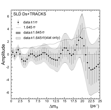
Figure 2: Measured $B_{s}^{0}$ oscillation amplitude as a function of $\Delta m_{s}$. The light-grey (dark-grey) band shows the 90% confidence region obtained from statistical (total) uncertainties. Values of $\Delta m_{s}$ for which the allowed band is below $A=1.0$ are excluded at the one-sided 95% confidence level.

There is no evidence for a significant signal anywhere in the plot, so we use the analysis to set a limit on $\Delta m_{s}$. The systematic errors on $A$ are evaluated according to reference Moser , all of which are negligible compared to the statistical errors. The systematics are dominated by uncertainties in a small reconstructed proper time bias (evaluated at 100% of the simulated correction, typically a few hundreths of a picosecond), in the production flavor tag (evaluated with $\pm 0.8$% uncertainty in the average tag probability and a reweighting of the shape of the distribution as a function of neural net output), in $f_{D_{s}^{-}}$ (as determined from the $KK\pi$ mass fit), and in the boost resolution (10%). To a lesser extent, there are contributions from uncertainties in decay length resolution (7%) and branching fractions assumed in the fit. Uncertainties in particle lifetimes and in the $B_{d}^{0}$ oscillation frequency are completely negligible. The list of systematic errors is shown in Table 2. The dark-grey band in Figure 2, barely visible at the edge of the light-grey band, shows the effect of adding the total systematic error to the calculations.

Table 1: $B$ production fractions and various branching ratios assumed in the amplitude fit. The uncertainties for the branching ratios do not include the uncertainty from ${\cal B}$($D_{s}\rightarrow~{}\phi\pi$).

Parameter	Value and Error	Ref.
f($\overline{b}\rightarrow B_{s}^{0}$)	$0.100\pm 0.012$	WORKG
f($\overline{b}\rightarrow B_{d}^{0},B^{+}$)	$0.401\pm 0.010$	WORKG
f($\overline{b}\rightarrow b-baryon$)	$0.099\pm 0.017$	WORKG
$R_{b}\cdot{\it f}(b\rightarrow\overline{B_{s}^{0}})\cdot{\cal B}(\overline{B_{s}^{0}}\rightarrow D_{s}^{+}X)\cdot{\cal B}(D_{s}^{+}\rightarrow\phi\pi^{+})$	$(6.21^{+0.71}_{-0.78})\times 10^{-4}$	WORKG ; ALEPH1
${\it f}(b\rightarrow W^{-}\rightarrow D_{s}^{-})\cdot{\cal B}(D_{s}^{-}\rightarrow\phi\pi^{-})$	$(3.66\pm 0.45)\times 10^{-3}$	ALEPH1
${\cal B}(B_{d}^{0},B^{+}\rightarrow D_{s}^{\pm}X)\cdot{\cal B}(D_{s}^{-}\rightarrow\phi\pi^{-})$	$(3.71\pm 0.28)\times 10^{-3}$	WORKG
${\cal B}(B_{d}^{0},B^{+}\rightarrow D_{s}^{-}X)/{\cal B}(B_{d}^{0},B^{+}\rightarrow D_{s}^{\pm}X)$	$0.172\pm 0.083$	WORKG
${\cal B}(\overline{c}\rightarrow D_{s}^{-})\cdot{\cal B}(D_{s}^{-}\rightarrow\phi\pi^{-})$	$(3.4\pm 0.3)\times 10^{-3}$	WORKG

Table 2: Table of statistical and dominant systematic uncertainties for several $\Delta m_{s}$ values.

$\Delta m_{s}$	10 ps-1	15 ps-1	20 ps-1
Measured amplitude $A$	0.029	$1.027$	$2.513$
$\sigma_{A}^{stat}$	$\pm 0.933$	$\pm 1.361$	$\pm 2.283$
$\sigma_{A}^{syst}$	${}^{+0.088}_{-0.084}$	${}^{+0.312}_{-0.313}$	${}^{+0.776}_{-0.789}$
f($\overline{b}\rightarrow B_{s}^{0}$)	${}^{+0.012}_{-0.012}$	${}^{+0.021}_{-0.022}$	${}^{+0.010}_{-0.011}$
f($\overline{b}\rightarrow b-$baryon)	${}^{+0.004}_{-0.004}$	${}^{+0.001}_{-0.001}$	${}^{-0.019}_{+0.019}$
$R_{b}\cdot{\cal B}(b\rightarrow\overline{B_{s}^{0}})\cdot{\cal B}(\overline{B_{s}^{0}}\rightarrow D_{s}^{+}X)$	${}^{-0.032}_{+0.043}$	${}^{-0.040}_{+0.048}$	${}^{-0.068}_{+0.068}$
${\cal B}(b\rightarrow W^{-}\rightarrow D_{s}^{-})$	${}^{+0.013}_{-0.013}$	${}^{+0.022}_{-0.022}$	${}^{+0.010}_{-0.012}$
${\cal B}(B_{d}^{0},B^{+}\rightarrow D_{s}^{\pm}X)$	${}^{+0.013}_{-0.014}$	${}^{+0.013}_{-0.014}$	${}^{+0.042}_{-0.047}$
$\frac{{\cal B}(B_{d}^{0},B^{+}\rightarrow D_{s}^{-}X)}{{\cal B}(B_{d}^{0},B^{+}\rightarrow D_{s}^{\pm}X)}$	${}^{+0.012}_{-0.013}$	${}^{+0.058}_{-0.060}$	${}^{+0.153}_{-0.156}$
${\cal B}(\overline{c}\rightarrow D_{s}^{-})$	${}^{+0.003}_{-0.003}$	${}^{+0.007}_{-0.007}$	${}^{+0.011}_{-0.011}$
Decay length resolution	${}^{+0.034}_{-0.036}$	${}^{+0.015}_{-0.015}$	${}^{+0.026}_{-0.045}$
Boost resolution	${}^{+0.049}_{-0.048}$	${}^{-0.052}_{+0.042}$	${}^{-0.161}_{+0.140}$
${\it f}_{D_{s}}$	${}^{+0.019}_{-0.018}$	${}^{+0.096}_{-0.096}$	${}^{-0.090}_{+0.076}$
Average production flavor tag	${}^{-0.029}_{+0.031}$	${}^{-0.036}_{+0.036}$	${}^{-0.051}_{+0.048}$
Production flavor tag shape	${}^{-0.020}_{+0.018}$	${}^{+0.008}_{-0.013}$	${}^{+0.306}_{-0.318}$
Proper time offset	${}^{+0.007}_{-0.007}$	${}^{+0.278}_{-0.278}$	${}^{+0.671}_{-0.671}$

Based on the result of the amplitude fit, the values of the $B_{s}^{0}$ oscillation frequency excluded at the 95% confidence level are: $\Delta m_{s}<1.4$ ps^-1 and $2.4<\Delta m_{s}<5.3$ ps^-1.

V Conclusions

In conclusion, we have performed a search for $B_{s}^{0}-\overline{B_{s}^{0}}$ oscillations using 361 $B_{s}^{0}\rightarrow D_{s}^{-}X$ candidate events with an average $B_{s}^{0}$ purity of 40%. The excluded values of oscillation frequency are: $\Delta m_{s}<1.4$ ps^-1 and $2.4<\Delta m_{s}<5.3$ ps^-1 at the 95% confidence level. The analysis exploits the unique large polarized forward-backward asymmetry in $Z^{0}\rightarrow b\bar{b}$ decays to enhance the production flavor tag. Combining the good production flavor tag and excellent proper time resolution, the analysis contributes to the world average at high $\Delta m_{s}$ despite low statistics. Taken in conjunction with other published results, our result raises the 95% C.L. world limit on $\Delta m_{s}$ from 13.1 ps^-1 to 13.9 ps^-1.

References

- (1) D.E. Groom et al., The European Physical Journal 15 (2000) 1 and 2001 off-year partial update for the 2002 edition available on the PDG WWW pages (URL:http://pdg.lbl.gov/).
- (2) C. W. Bernard, Nucl. Phys. B Proc. Suppl. 94, 159 (2001).
- (3) The small theoretical error in the ratio of to oscillation frequency quoted in the previous reference has recently been challenged. See A. S. Kronfeld and S. M. Ryan, arXiv:hep-ph/0206058.
- (4) M. Ciuchini et al., JHEP 0107, 013 (2001).
- (5) C-J. S. Lin, Ph.D. Dissertation, University of Massachusetts, Amherst, MA (2001), SLAC-R-584.
- (6) Charge conjugate reactions are implied throughout this paper.
- (7) SLD Design Report, SLAC Report 273 (1984).
- (8) P. Rowson, D. Su, S.Willocq, Ann. Rev. Nucl. Part. Sci. 51, 345 (2001).
- (9) D. J. Jackson, Nucl. Inst. and Meth. A388, 247 (1997).
- (10) K. Abe et al. [SLD Collaboration], SLAC-PUB-8542, July 2000.
- (11) A. S. Chou, Ph. D. Dissertation, Stanford University, Stanford, CA (2001), SLAC-R-578.
- (12) T. B. Moore, Ph.D. Dissertation, Yale University, New Haven, CT (1999).
- (13) K. Abe et al. [SLD Collaboration], Phys. Rev. D65, 092006 (2002).
- (14) H.G. Moser and A. Roussarie, Nucl. Inst. Meth., A384, 491 (1997).
- (15) ALEPH, DELPHI, L3, OPAL, CDF, and SLD Collaborations, Combined results on b-hadron production rates, lifetimes, oscillations and semileptonic decays, CERN-EP-2000-096, SLAC-PUB-8492.
- (16) D. Buskulic et al. [ALEPH Collaboration], Z. Phys. C 69, 585 (1996).