Atmospheric gamma-ray observation with the BETS detector for calibrating atmospheric neutrino flux calculations

Abstract

We observed atmospheric gamma-rays around 10 GeV at balloon altitudes (15$\sim$25 km) and at a mountain (2770 m a.s.l). The observed results were compared with Monte Carlo calculations to find that an interaction model (Lund Fritiof1.6) used in an old neutrino flux calculation was not good enough for describing the observed values. In stead, we found that two other nuclear interaction models, Lund Fritiof7.02 and dpmjet3.03, gave much better agreement with the observations. Our data will serve for examining nuclear interaction models and for deriving a reliable absolute atmospheric neutrino flux in the GeV region.

I Introduction

The discovery of evidence for neutrino oscillation by the Super Kamiokande groupFukuda et al. (1998) is based on the comparison of the observed atmospheric neutrino flux with calculated values. Although the conclusion is so derived that it would not be upset by the uncertainty of the absolute flux value, it is desirable to obtain a reliable expected neutrino flux (under no oscillation assumption) for further detailed discussions.

Two major sources of uncertainty in the atmospheric neutrino flux calculation are 1) the primary cosmic-ray spectrum and 2) the propagation of cosmic rays in the atmosphere, especially, modeling of the nuclear interaction. The absolute flux calculations so far made by various groups are expected to have uncertainty of $\sim$ 30 %Gaisser and Honda (2002).

The primary proton and He spectra recently measured with magnet spectrometers by the BESS Sanuki et al. (2000) and AMSAMS collaboration (2000) groups agree very well and seem reliable. Therefore, we may take that the first problem mentioned above have now been almost settled at least up to 100 GeV/n. This means that if we have a reliable atmospheric cosmic-ray flux data, we may compare it with a calculation which uses such primaries and test the validity of nuclear interaction models.

For such an atmospheric cosmic-ray component, one may first raise the muon and actually some new observations have been or being triedKremer et al. (1999); Circella et al. (2001); Sanuki et al. (2002).

As a secondary cosmic-ray component, we focused on gamma-rays which are easy to measure with our detector. A good model should be able to explain muons and gamma-rays simultaneously. Muons are important since they are directly coupled with neutrinos, but the flux is affected somehow by the structure of the atmosphere which is usually not well known. Compared to muons, the flux of gamma-rays is substantially lower but is almost insensitive to the atmospheric structure and depends only on the total thickness to the observation height.

In 1998, we performed first gamma-ray observation with our detector at Mt. Norikura (2770m a.s.l) in Japan, and also made subsequent two successful observations at balloon altitudes (15 $\sim 25$ km) in 1999 and 2000. In the present paper, we report the final results of these observations and consequences.

II The Detector

For our observation, we upgraded the BETS (Balloon-born Electron Telescope with Scintillating fibers) detector which had been developed for the observation of cosmic primary electrons in the 10 GeV region. Its details before being upgraded for gamma-ray observation is in Torii et al. (2000a) and the electron observation result is in Torii et al. (2001). The basic performance was tested at CERN using electron, proton and pion beams of 10 to 200 GeVTorii et al. (2000a); Tamura et al. (1999). Although this was undertaken before the upgrading, we can essentially use that calibration for the current observeions partly with a help of Monte Carlo simulations.

Figure 1 shows a schematic structure of the main body of BETS. The calorimeter has 7.1 r.l lead thickness and the cross-section is 28 cm $\times$ 28 cm. The whole detector system is contained in a pressure vessel made of thin aluminum.

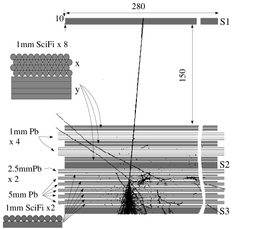
Figure 1: Schematic illustration of the main body of the detector. S1, S2 and S3 are 1 cm thick plastic scintillators used for trigger. Each fiber has 1mm diameter. Originally nuclear emulsion plates were placed on the upper scifi’s and also inserted between the upper thin lead plates for detailed investigation of tracking capability of scifi. They are kept in the present system to have the same structure at the calibration time. The inlaid cascade shows charged particle tracks by a simulation for a 30 GeV incident proton.

Table 1: Basic characteristics of BETS
(triple numbers in the table are for gamma-ray energy of 5, 10, and 30 GeV, respectively)

R.M.S energy resolution(%)	21, 18, 15 (for $\theta\sim 15^{\circ}$)
S$\Omega$(cm2sr)	243, 240,218 (at $\sim$20 km)
R.M.S angular resolution (deg)	2.3, 1.3, 1.0 (for $\theta\sim 15^{\circ}$)
Total number of scifi’s	10080
Weght including electronics (kg)	230
Cross-section of the main body	28cm $\times$ 28cm
Thickness (Pb radiation length)	7.1

The main feature of the BETS detector is that it is a tracking calorimeter; it contains a number of sheets consisting of 1 mm diameter scintillating fibers (scifi), many of which are sandwiched between lead plates. The total number of scifi’s are 10080. The sheets are grouped into two types; one is to serve for x and the other for y position measurement. Each of them is fed to an image intensifier which in turn is connected to a CCD. Thus, the two CCD output gives us an $x-y$ image of cascade shower development and enables us to discriminate gamma-rays, electrons from other (mainly hadronic) background showers. The proton rejection power against electron is $R\sim 2\times 10^{3}$ (i.e, one misidentification among $R$ protons) at 10 GeV The basic characteristics of the detector are summarized in Table 1.

Figure 2: Image of cascade shower by a proton (120 GeV,left) and an electron(10 GeV, right) obtained at CERN.

In Fig.2, we show examples of the CCD image of a cascade shower for a proton incident case and for an electron incident case.

Figure 3 illustrates the yearly change of anti-counters. In 1998 (Mt.Norikura observation), the main change was limited to the upgrading of trigger logic. In 1999, we added 4 side anti-counters (each 15 cm $\times$ 36 cm $\times$ 1.5 cm plastic scintillator. Nine optical fibers containing wave length shifter are embedded in each scintillator and connected to a Hamamatu H6780 PMT.

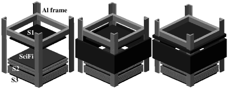
Figure 3: Yearly change of the anti-counters. Left: 1998. No change from original BETS except for trigger logic. Middle: 1999. 1.5 cm thick plastic scintillator side anti-counters were added. Right: 2000. The whole top view was covered by a 1 cm thick plastic sintillator.

In 2000, we further added an anti-counter which covers the whole top view of the detector and also improved data acquisition speed. The top anti-counter is 38 cm $\times$ 38 cm $\times$ 1 cm plastic scintillator. We also embedded optical fibers; 8 in the $x$ and another 8 in the $y$ direction, all of which were fed to an H6780.

Although we could remove background showers without the anti-counters, inclined particles (mainly protons) entering from the gap between top scintillator (S1) and the main body degrades the desired gamma-ray event rate. The addition of the top anti-counter greatly helped improve this rate.

We emphasize that detection of gamma-rays is easier for us than that of electrons, since, for gamma-rays, we can utilize absence of incident charge.

III Observations

Table 2 shows the summary of the observations.

Table 2: Summary of three observations

Observation	Mt.Norikura(1998)	Balloon (Sanriku, 1999)					Balloon (Sanriku, 2000)
Period	Aug.31$\sim$Sep.18	Sep.2, 6:55$\sim$17:17					Jun.5, 6:30$\sim$17:59
Altitude(km)	2.77	15.3	18.5	21.2	24.7	32.3	15.3	18.3	21.4	25.1
Depth(g/cm2)	737	126	74.8	48.9	28.0	9.5	128	73	45.7	25.3
Obs. hour (s)	$1.33\times 10^{6}$	1260	1560	2100	4878	3120	1560	2160	4320	2320
Live time (s)	$9.8\times 10^{5}$	504	450	414	852	498	752	928	1805	789
Live time (%)	74.0	40.0	28.8	19.7	17.5	16.0	48.2	43.0	42.6	44.2
Triggered events	$1.8\times 10^{6}$	9513	11288	13361	30439	16741	18808	25795	46675	17436
$\gamma$ events	$4.7\times 10^{4}$	700	650	611	848	345	1300	1485	2299	740
(%)	2.5	7.3	5.7	4.6	2.8	2.0	6.9	5.8	4.9	4.2
g-low trigger	S1 $<0.5$	S1$<0.5$					S1$<0.47$
condition (in mip).	S2 $>2.3$	S2$>1.5$					S2$>1.59$
	S3 $>1.7$	S3$>3.0$					S3$>3.18$

• Mt. Norikura observation.

  Our first gamma-ray observation was performed in 1998 at Mt.Norikura Observatory of Univ. of Tokyo, Japan (2770 m a.s.l, latitude 36.1^∘N, longitude 137.55^∘E, magnetic cutoff rigidity $\sim$ 11.5 GV). The atmospheric pressure during the observation is shown in Fig.4. The average atmospheric depth is 737 g/cm².

  

  Figure 4: Pressure change during Mt. Norikura observation. The last pressure drop is due to a typhoon. The average pressure is 723 hP (737 g/cm²).

• Balloon flight

  We had two similar balloon filights in 1999 and 2000. Since the main outcome of the data is from the latter, we briefly describe it. A balloon of 43$\times 10^{3}$ m³ was launched at 6:30 am, 5th June, 2000 from the Sanriku balloon center of the Institute of Space and Astronautical Science, Japan (latitude 39.2^∘N, longitude 141.8^∘E, magnetic cutoff rigidity $\sim$ 8.9 GV) and recovered with the help of the helicopter. at 17:59 on the sea not far from the center. The flight curve shown in Fig.5 confirms that we have good level flights at 4 different heights.

  As compared to the 1999 flight, this flight realized a smaller dead time and higher ratio of desired gamma-ray events.

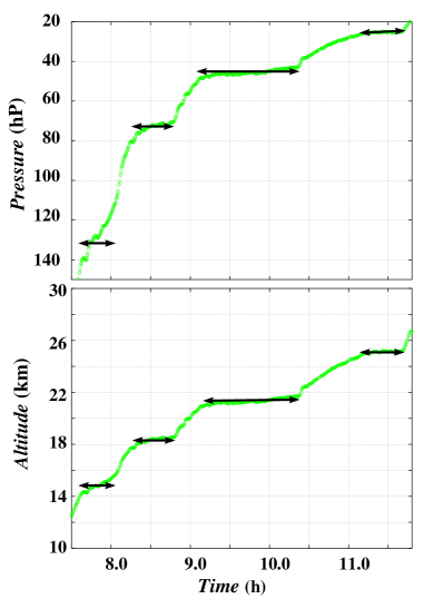
Figure 5: Flight curve of the 2000 observation. Pressure (upper) and altitude (lower) as a function of time. Each arrow shows the level flight region. The pressure change at around 15.3 km is rather rapid but the gamma-ray intensity is almost constant there and the change can be neglected.

III.1 Event trigger

The basic event trigger condition is created by signals from the three plastic scintillators (S1, S2 and S3). We show the discrimination level in terms of the minimum ionizing particle number which is defined by the peak of the energy loss distribution of cosmic-ray muons passing both S1 and S3 with inclination less than 30 degrees.

We prepare a multi-trigger system by which event trigger with different conditions is possible at the same time. The major two trigger modes are the g-low and g-high. The g-low is responsible for low energy gamma-rays and all anti-counters, when available, are used as veto counters. Its condition is listed in Table 2. High energy gamma-rays normally produce a lot of back splash particles which hit S1 and/or anti-counters, and thus the g-low trigger is suppressed. In such a case, i.e, if we have a large S3 signal, anti-counter veto is invalidated and the S1 threshold is relaxed (The g-high condition is S1$<3.0$, S2$>5.0$ and S3$>8.1$).

The branch even point of the g-low and g-high mode efficiency is at $\sim$30 GeV. Since we deal with gamma-rays mostly below 30 GeV, and also to avoid complexity, we present results only by the g-low mode.

IV Analysis

IV.1 Event selection

Among the triggered events, we selected gamma-ray candidates by imposing the following conditions:

Figure 6: (left)Energy concentration distribution at 21.4 km. (right)the same by electrons at CERN

1. The estimated shower axis passes S1 and S3. The axis position in S3 must be at least 2 cm apart from the edge of S3.

2. The estimated shower axis has a zenith angle less than 30 degrees.

3. The energy concentration (see below) must be greater than 0.7.

According to a simulation, only neutrons could be a background against gamma-rays and the 3rd conditions above reduces the neutron contribution to a negligible level ($<1$%).

The energy concentration is defined as the fraction of scintillating fiber light intensity within 5 mm from the shower axis. Figure 6 shows the concentration of analysed events together with the result of CERN data. Hadrons make a distribution with a peak at around 0.5. We see that the contribution of hadrons in our observation is negligible.

IV.2 Energy Determination

The energy calibration was performed in 1996 at CERN using electrons with energy 10 $\sim$ 200 GeVTorii et al. (2000a); Tamura et al. (1999). There is no direct calibration for gamma-rays, but, for the present detector thickness and energy range, a M.C simulation tells us that the calibration in 1996 can be used for gamma-rays, too. Therefore, for the 1998 and 1999 observations, energy is obtained as a function of the S3 output and zenith angle using the CERN calibration.

In 2000, we made some change in the electronics so the CERN calibration could not be used directly. The effect by the change was absorbed by a M.C simulation of which the validity was verified by examining the 1998 and 1999 data. We used the sum of S2 and S3 outputs below 20 GeV since the energy resolution was found to be better than using S3 only. Figure 7 shows r.m.s energy resolution.

Figure 7: R.m.s energy resolution. The resolution by S2+S3 or S3 only is shown. Different symbols indicate different incident angles. We used S2+S3 below 20 GeV for the year 2000 data.

IV.3 Correction of the gamma-ray intensity

The gamma-ray vertical flux is obtained from the raw $dN/dE$ by dividing it by the live time of the detector and the effective $S\Omega$ (area $\times$ solid angle). The latter is obtained by a simulationTorii et al. (2000b). It is dependent on the observation hight and energy. A typical value at 10 GeV is 240 cm²sr (see Table1). The energy spectrum is further corrected by the following factors which are not taken into account in the $S\Omega$ calculation.

Figure 8: (upper)Multiple incidence rate. (lower) Correction factor for year 2000 due to spillover. The flux must be lowered. For Norikura, the factor below 20 GeV is larger by 1$\sim 3$ %.

1. Systematic bias in our estimation of the shower axis. We underestimate the zenith angle systematically and it leads to overestimation of the intensity about 4% for the balloon and 1.8 % for Mt.Norikura observations.

2. Multiple incidence of particles. A gamma-ray is sometimes accompanied by other charged particles and they enter the detector simultaneously (within 1 ns time difference in 99.9 % cases). They are a family of particles generated by one and the same primary particle. The charged particles fire the anti-counter and the g-low trigger is inhibited.

   In some case, multiple gamma-rays enter the detector simultaneously. The rate is smaller than the charged particle case. However, this is judged as a hadronic shower in most of cases. The multiple incidence leads to the underestimation of gamma-ray intensity. The portion of multiple incidence is shown in Fig.8 (upper).

3. Finite energy resolution. The rapidly falling energy spectrum leads to the spillover effect. This normally leads to the overestimation of flux (Fig.8, lower).

V Results and comparison with calculations

The flux values are summarized in Table 3. We put only the statistical errors in the flux values, since systematic errors coming from the uncertainty of the S$\Omega$ calculation, various cuts and flux corrections are expected to be order of a few percent and much smaller than the present statistical errors.

Table 3: Summary of flux values

height (km)
15.3		18.3		21.4		25.1		32.3
Energy (GeV)  &  flux(No./$m^{2}\cdot$ s$\cdot$sr$\cdot$GeV)
5.48	2.42 $\pm$ 0.37	5.48	2.11 $\pm$ 0.39	5.47	2.11 $\pm$ 0.24	5.47	1.58 $\pm$ 0.25	5.47	0.49 $\pm$ 0.14
6.47	1.18 $\pm$ 0.27	6.47	1.10 $\pm$ 0.24	6.47	1.35 $\pm$ 0.21	6.47	0.82 $\pm$ 0.18	6.57	0.19 $\pm$ 0.09
7.47	0.89 $\pm$ 0.24	7.47	0.79 $\pm$ 0.21	7.47	0.82 $\pm$ 0.16	7.47	0.66 $\pm$ 0.16	7.47	0.24 $\pm$ 0.10
8.48	0.37 $\pm$ 0.15	8.48	0.92 $\pm$ 0.20	8.48	0.51 $\pm$ 0.13	8.48	0.49 $\pm$ 0.14	8.48	0.16 $\pm$ 0.08
9.48	0.54 $\pm$ 0.17	9.85	0.46 $\pm$ 0.11	9.48	0.50 $\pm$ 0.12	9.48	0.36 $\pm$ 0.12	9.48	0.16 $\pm$ 0.08
10.5	0.17 $\pm$ 0.10	11.5	0.35 $\pm$ 0.12	10.5	0.41 $\pm$ 0.09	10.5	0.34 $\pm$ 0.12	12.3	0.13 $\pm$ 0.037
12.1	0.28 $\pm$ 0.09	14.0	0.24 $\pm$ 0.06	11.8	0.23 $\pm$ 0.069	12.2	0.21 $\pm$ 0.054	17.0	0.032 $\pm$ 0.018
14.0	0.17 $\pm$ 0.05	18.3	0.072 $\pm$ 0.030	14.0	0.16 $\pm$ 0.030	14.0	0.076 $\pm$ 0.03	21.7	0.022$\pm$ 0.015
18.5	0.12 $\pm$ 0.04	26.8	0.040 $\pm$ 0.017	18.4	0.086 $\pm$ 0.023	17.8	0.078 $\pm$ 0.029
25.5	0.06 $\pm$ 0.02			27.1	0.026 $\pm$ 0.009	21.7	0.064 $\pm$ 0.026
						26.8	0.024 $\pm$ 0.012
						36.0	0.012 $\pm$ 0.008

Table 4: Flux values at Mt. Norikura

E(GeV)	Flux ($10^{-4}/$m${}^{2}\cdot$s$\cdot$sr$\cdot$GeV)
5.48	274 $\pm$ 13
6.47	183 $\pm$ 11
7.47	133 $\pm$ 9
8.47	87.8 $\pm$ 7.5
9.47	86.5 $\pm$ 7.5
10.5	54.1 $\pm$ 5.9
11.5	46.6 $\pm$ 5.5
12.5	38.3 $\pm$ 5.0
13.5	32.6 $\pm$ 4.6
14.5	24.2 $\pm$ 4.0
15.5	25.7 $\pm$ 4.1
17.0	11.9 $\pm$ 2.0
19.0	15.3 $\pm$ 2.3
21.0	13.1 $\pm$ 2.1
23.0	5.80 $\pm$ 1.4
26.0	5.31 $\pm$ 0.95
30.0	3.00 $\pm$ 0.72
34.0	2.30 $\pm$ 0.64
38.0	1.07 $\pm$ 0.44
45.0	1.45 $\pm$ 0.32
55.0	0.52 $\pm$ 0.20
65.0	0.22 $\pm$ 0.13
75.0	0.30 $\pm$ 0.15
85.0	0.15 $\pm$ 0.10

The gamma-ray energy spectra thus obtained at balloon altitudes are shown in Fig.9 together with the expected ones calculated by the Cosmos simulation codecos . Except for 32.3 km altitude, we can disregard the small difference of the observation depths and we combine two flight data with statistical weight, although the main contribution is from the flight in 2000.

In the simulation calculation, we employed 3 different nuclear interaction models: 1) fritiof1.6Almqvist and Stenlund (1987) used in the HKKM calculationHonda et al. (1995), which was widely used for comparison with the Kamioka data, 2)fritiof7.02Pi (1992) and 3) dpmjet3.03Roesler et al. (2000). As the primary cosmic ray, we used the BESS result on protons and He. The CNO component is also consideredCompilation by J. A. Simpson (1982). Besides these we included electron and positron data by AMSAMS Collaboration (2000). Their data in the 10 GeV region is consistent with the HEATBarick et al. (1998) and BETSTorii et al. (2001) data. Bremstrahlung gamma-rays from the primary electrons could contribute order of $\sim 10$ % at very high altitudes.

At balloon altitudes, the two models, fritiof7.02 and dpmjet3.03, give almost the same results which are close to the observed data, while fritof1.6 gives clearly smaller fluxes than the observation.

Figure 10 shows the result from the observation at Mt.Norikura. It should be noted that the flux by fritiof1.6 becomes higher than the ones by the other models at this altitude.

From these figures, we see fritiof7.02 and dpmjet3.03 give rapider increase and faster attenuation of intensity than fritiof1.6; the tendency is very consistent with the observed data. The transition curve of the flux integrated over 6 GeV shown in Fig.11 clearly demonstrates this feature.

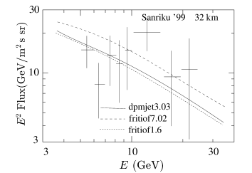
Figure 9: Gamma-ray spectra at 5 balloon heights are compared with 3 different models. The vertical axis is Flux$\times E^{2}$. Except for 1999 data at 32.3 km, 1999 and 2000 flights data are combined. From top to bottom, at 25.1, 21.4, 18.3, 15.3 and 32.3 km. The spectra expected from three interaction models are drawn by solid (dpmjet3.03), dash (fritiof7.02) and dotted (fritiof1.6) lines.

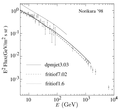
Figure 10: Gamma-ray spectrum at Mt. Norikura (2.77 km a.s.l). The vertical axis is Flux$\times E^{2}$. Our data is at $<$ 100 GeV. Data above 300 GeV is from emulsion chamber experiments. For the latter, see Sec.VI

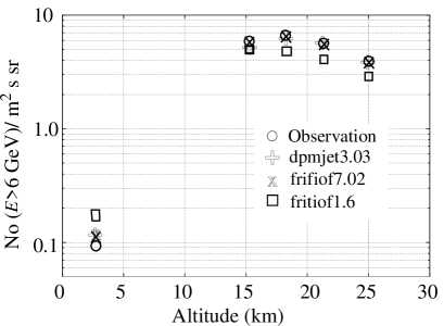
Figure 11: The altitude variation of the flux integrated over 6 GeV. The dpmjet3.03 and fritiof7.02 give almost the same feature consistent with the observation while the deviation of fritiof1.6 from the data is obvious.

VI Discussions

VI.1 Comparison with other data

We found Fritiof7.02 and dpmjet3.03 give good agreement with the observed gamma-ray data at around 10 GeV. We briefly see whether these models can interpret other observations. More detailed inspection will be done elsewhere.

• Muon data by the BESS group at Mt.NorikuraSanuki et al. (2002).

  Recently, the BESS group reported detailed muon spectrum over several hundred MeV/c. In their paper, calculations by dpmjet3.03 and fritiof1.6 are compared with the data; agreement by dpmjet3.03 is quit good at least above GeV where Fritiof7.02 also gives more or less the same flux. On the other hand, fritiof1.6 shows too high flux. These features are consisten with our present analysis.

• Higher energy gamma-ray data by emulsion chamber.

  In Fig. 10, we inlaid an emulsion chamber dataAkashi et al. (1964) at Mt. Norikura. Our data seems to be smoothly connected to their data as the two interaction models (Fritiof7.02 and dpmjet3.03) predict. Since the emulsion chamber data extends to the TeV region and the primary particle energy responsible for such high energy gamma-rays is much higher than 100 GeV where we have no accurate information comparable to the AMS and BESS data, it would be premature to draw a definite conclusion on the primary and interaction model separately. However, the fact that smooth extrapolation of the primary spectra as shown in Table 5 and the interaction model, dpmjet3.03 or fritiof7.02, give a consistent result with the data, seems to indicate that such combination would provide a good estimate on other components at $\gg$ 10 GeV.

  Table 5: Primary flux assumed in the simulation above 100 GeV/n
  (E in kinetic energy per nucleon (GeV), flux in /m${}^{2}\cdot$s$\cdot$sr$\cdot$GeV)

  Proton		Helium		CNO
  E	flux	E	flux	E	flux
  92.6	0.593E-01	79.4	0.549E-02	100.	9.0E-5
  108	0.388E-01	100.	3.0E-3	400.	1.8E-6
  126	0.276E-01	200.	5.0E-4	2.0E3	3.5E-8
  147	0.179E-01	400.	7.0E-5	2.0E4	9.3E-11
  171	0.124E-01	2.0E3	9.98E-7	2.0E5	2.3E-13
  200	0.836E-02	2.0E4	2.5E-9	14.0E5	1.3E-15
  1100	8.29E-5	2.0E5	3.97E-12	3.0E6	1.7E-16
  1.1E4	1.47E-7	4.0E5	6.1E-13	3.0E7	2.0E-19
  1.1E5	2.8E-10	8.0E5	7.0E-14	3.0E8	2.2E-22
  2.2E5	3.7E-11	8.0E6	8.7E-17
  4.4E5	5.0E-12	8.0E8	5.3E-23
  4.4E8	2.8E-21

VI.2 The $x$-distributions

The two models, fritiof7.02 and dpmjet3.03, give almost the same results in the present comparison. However, if we look into the $x$-distribution of the particle production, we note some difference, especially in the proton $x$-distribution. We define the $x$ as the kinetic energy ratio of the incoming proton and a secondary particle in the laboratory frame. The $x$ distribution for $p$Air collisions at incident proton energy of 40 GeV is presented for photons (from $\pi^{0}$ plus $\eta$ decay) and protons in Fig.12. Difference of the three models seen in the photon distribution is quite similar to the one for charged pions. The $x$ region most effective to atmospheric gamma-ray flux is around 0.2$\sim$0.3 where the difference is not so large but fritiof7.02 and dpmjet3.03 have higher gamma-ray yield than fritiof1.6.

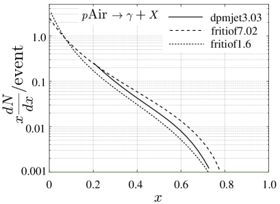
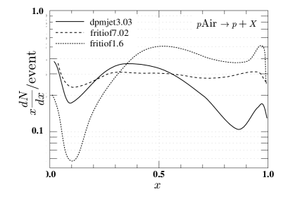
Figure 12: The $x$-distribution of photons from $\pi^{0}$ plus $\eta$ decay (upper) and protons (lower) for $p$Air collisions at 40 GeV. The three model results are shown.

On the other hand, the proton $x$ distribution has larger difference among the three models (we note, however, the difference may be exaggerated than the photon case due to the scale difference). It is interesting to see that, in spite of these large differences, the final flux is not so much different each other. Our gamma-ray data prefers to rather more inelastic feature of collisions than fritiof1.6, i.e rapider increase and faster attenuation of the flux.

We should compare the distribution with accelerator data; however, there is meager stuff appropriate for our purpose. One such comparison has been done in a recent review paperGaisser and Honda (2002) for $p$Air collisions at 24 GeV/c incident momentum. The charged pion distribution by fritiof1.6 and dpmjet3.03 well fit to some scattered data which prevents to tell the superiority of the two. As to the proton distribution, among the three models, fritiof1.6 is rather close to the data but deviation from the data is much larger than the pion case.

The proton $x$-distribution would strongly affect the atmospheric proton spectrum. We calculated proton flux at Mt.Norikura to find a flux relation such that fritiof1.6 $>$ fritiof7.02 $>$ dpmjet3.03 as expected naturally from the $x$-distributions. The maximum difference is factor $\sim 2.5$ in the energy region of 0.3 to 3 GeV. The BESS group has measured the proton spectrum at Mt. Norikura in the same energy region. Their result expected to come soonSanuki will help select a better model for the proton $x$ distribution.

VII summary

• We have made successful observation of atmospheric gamma-rays at around 10 GeV at Mt.Norikura (2.77 km a.s.l) and at balloon altitudes (15 $\sim$ 25 km).

• The observed gamma-ray fluxes are compared with calculations by three interaction models; it is found that fritiof1.6 employed by the HKKM calculation Honda et al. (1995), which was used in comparison with the Kamioka data, is not a very good model.

• Other two models (fritiof7.02 and dpmjet3.03) give better results consistent with the data, which shows rapider increase and faster attenuation of the flux than fritiof1.6 predicts.

• Our data has complementary feature to muon data and will serve for checking nuclear interaction models used in atmospheric neutrino calculations.