Recent Results in Search for New Physics at the Tevatron (Run 1)

Abstract

We present some new results on searches for new physics at the Tevatron Run 1 (1992 – 1996). The topics covered are searches for R-Parity violating and conserving mSUGRA, large extra dimensions in di-photon and monojet channels, leptoquark in jets + ${\hbox{$E$\kern-6.00006pt\lower-0.43057pt\hbox{/}}}_{T}$ channel, and two model independent searches. All results were finalized during the past year.

1 Introduction

Tevatron Run I has been a great success for High Energy Physics. For the period between October 1992 and February 1996, about $120\;{\rm pb^{-1}}$ of data were collected by the two competing experiments and collaborations: CDF and DØ. Both collaborations have made many important measurements and discoveries with their powerful and multi-purpose detectors[1, 2], culminated by the discovery of the top quark in 1995. They are also engaged in search for new physics beyond the Standard Model (SM). Though no convincing evidence of new physics was found, the searches have extended our understanding of the fundamentals of the universe and have led our quest for ultimate understanding in a concerted direction.

This paper reports nine results on searches for new physics conducted recently at the Tevatron by CDF and DØ. We cover the topics of SUSY, large extra dimension, leptoquark, and model independent searches.

2 Search for mSUGRA

Minimal supergravity or mSUGRA[3] is a model which provides a framework for the spontaneous breaking of the supersymmetry[4]. In this model, SUSY is broken in the hidden sector of the theory and this breaking is communicated to the physical sector of the theory through gravitational interactions. There are five parameters to completely determine the SUSY sector of the theory:

• $m_{0}$: common scalar particle mass at the SUSY breaking scale $M_{X}$;

• $m_{1/2}$: common gaugino mass at the $M_{X}$ scale;

• $A_{0}$: common trilinear coupling at the $M_{X}$ scale;

• ${\rm tan}\beta$: ratio of the vacuum expectation values of the two Higgs doublets;

• ${\rm sign}(\mu)$: $\mu$ is the Higgsino mass parameter.

An additional parameter called R-Parity is introduced and is defined as: $R_{p}=-1^{3B+L+2S}$[5], where $B$ and $L$ are baryon and lepton numbers, respectively, and $S$ refers to spin. A superpotential for MSSM, the minimal supersymmetric extension of the standard model[6], can be written as the following:

$$W = \overline{u}{\rm\bf y_{u}}QH_{u}-\overline{d}{\rm\bf y_{d}}QH_{d}-\overline{e}{\rm\bf y_{e}}LH_{d}+\mu H_{u}H_{d}+$$ (1)

$$\lambda_{ijk}L^{i}L^{j}\overline{e}^{k}+\lambda^{\prime}_{ijk}L^{i}Q^{j}\overline{d}^{k}+\lambda^{\prime\prime}_{ijk}\overline{u}^{i}\overline{d}^{j}\overline{d}^{k}+\mu^{\prime}_{i}L^{i}H_{u}.$$

where the first line describes $R_{p}$-conserving couplings and the second line describes $R_{p}$-violating couplings; ${\rm\bf y_{u}}$, ${\rm\bf y_{d}}$, and ${\rm\bf y_{e}}$ are $3\times 3$ Yukawa coupling matrices; $Q$ and $L$ are left-handed quark and lepton supermultiplets, respectively; $\overline{u}$, $\overline{d}$, $\overline{e}$ are the right-handed singlets of the up and down type (s)quarks and (s)leptons, respectively; $H_{u}$ and $H_{d}$ are the two Higgs doublets; $\mu$ is the Higgsino mass parameter; $\lambda$, $\lambda^{\prime}$, and $\mu^{\prime}$ are the coupling strengths for lepton number violating interactions and $\lambda^{\prime\prime}$ is the coupling strength for baryon number violating interactions.

We describe in this paper four searches for mSUGRA under various additional constraints.

2.1 CDF RPV mSUGRA search in decays of stop pair

In this analysis, we assume that stop pair are produced through $R_{p}$-conserving processes and then decay through $R_{p}$-violating process: $\tilde{t}\overline{\tilde{t}}\rightarrow\overline{\tau}_{l}+b+\tau_{h}+\overline{b}+X$, where $\tau_{l}$ and $\tau_{h}$ are leptonically and hadronically decayed $\tau$, respectively. We also assume that $\lambda^{\prime}_{333}$ in Eq. (1) dominates the couplings.

The key to this analysis is the identification of $\tau_{h}$. The following criteria are used to select $\tau_{h}$:

• $\tau_{h}$ candidates are clusters with $P_{T}>15\;{\rm GeV}$ and $|\eta_{det}|<1.0$;

• Number of tracks and $\pi^{0}$’s in a narrow cone around a $\tau$ cluster candidate are consistent with those coming from a $\tau$;

• $E/p$ and isolation energy of tracks and reconstructed $tau$ mass are consistent with those of a $\tau$.

Figure 1 shows the number of tracks in a $\tau$ cone. The 1-prong and 3-prong structures of the $\tau$ candidates are prominent.

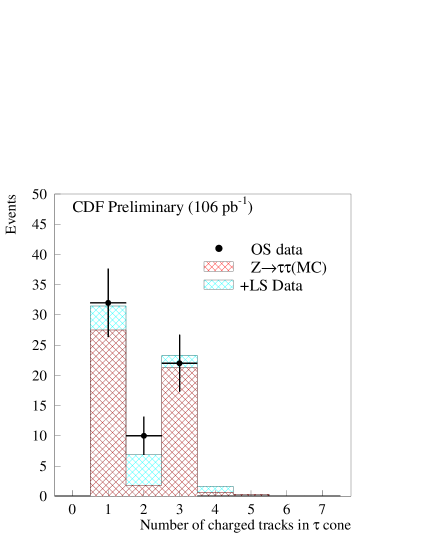
Figure 1: Number of tracks in a $\tau$ cone in $Z\rightarrow\tau\tau+0\;{\rm jet}$ events. Points are data. The darkly hatched histogram is the prediction from Monte Carlo, and the lightly hatched histogram is the estimation of background from data with like-sign charge. Charge of a $\tau$ candidate is the sum of track charges in the $\tau$ cone.

A total of $106\;{\rm pb^{-1}}$ of data are used in this analysis. The major SM backgrounds come from $Z,\gamma^{*}+{\rm jets}$, Diboson, $W(e\nu,\mu\nu)+{\rm jets}$, $W(\tau\nu)+{\rm jets}$, and multijet events. The first two are physics backgrounds which have the same final states as the signal while the rest are $\tau$ fakes of by jets.

Leptonically decayed $\tau_{l}$ is identified with a tagging electron or muon. We require $E^{e}_{T}>10\;{\rm GeV}$, $|\eta^{e}_{det}|<1.0$ for the electron channel or $P^{\mu}_{T}>10{\rm GeV/c}$, $|\eta^{\mu}_{det}|<1.0$ for the muon channel. In order to increase the signal significance, the following additional selection cuts are applied:

• transverse mass of the lepton and the ${\hbox{$E$\kern-6.00006pt\lower-0.43057pt\hbox{/}}}_{T}$: $M_{T}({\rm lepton,\mbox{${\hbox{$E$\kern-6.00006pt\lower-0.43057pt\hbox{/}}}_{T}$}})<35\;{\rm GeV/c^{2}}$;

• the scalar sum of $E_{T}$ of the lepton, $\tau_{h}$, and ${\hbox{$E$\kern-6.00006pt\lower-0.43057pt\hbox{/}}}_{T}$: $H_{T}({\rm lepton},\tau_{h},\mbox{\mbox{${\hbox{$E$\kern-6.00006pt\lower-0.43057pt\hbox{/}}}_{T}$}})>70\;{\rm GeV}$;

• ${\rm N_{jet}}\geq 2$ with $E^{\rm{jet}}_{T}>15\;{\rm GeV}$.

The distribution of these variables are shown in Figure 2.

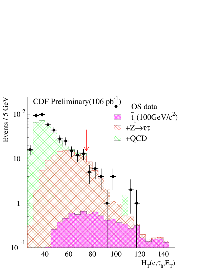
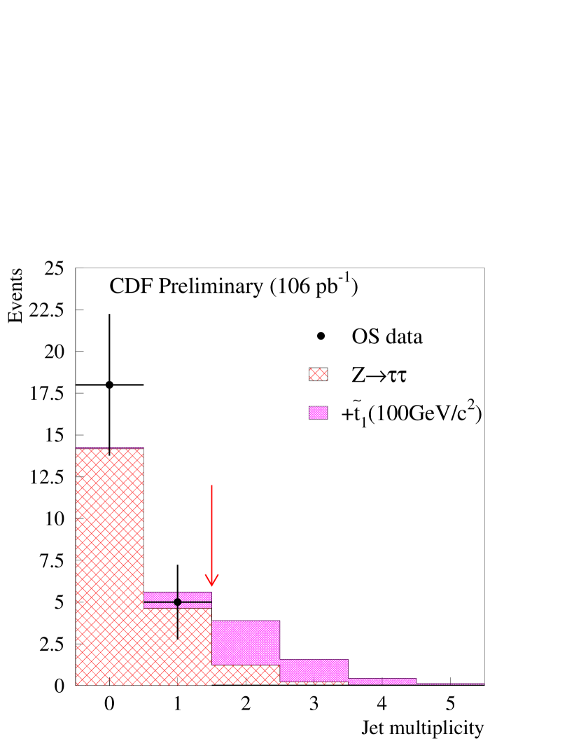
Figure 2: Distribution of $M_{T}({\rm electron,\mbox{${\hbox{$E$\kern-6.00006pt\lower-0.43057pt\hbox{/}}}_{T}$}})$ (top left), $H_{T}({\rm electron},\tau_{h},\mbox{\mbox{${\hbox{$E$\kern-6.00006pt\lower-0.43057pt\hbox{/}}}_{T}$}})$ (top right), and $N_{jet}$ (bottom) for signal and backgrounds in the electron channel of search for RPV mSUGRA in decays of stop pairs.

The results after the cuts are shown in Table 1. Since no signal is found in our data. We set the signal limit in terms of $\sigma_{\tilde{t}\overline{\tilde{t}}}$, the production cross section of $\tilde{t}\overline{\tilde{t}}$ as a function of $m_{\tilde{t}}$. The limits are shown in Figure 3. From the figure, we set the 95% C.L. limit on stop mass: $m_{\tilde{t}}>119\;{\rm GeV}$. The previous limit from ALEPH collaboration is $m_{\tilde{t}}>93\;{\rm GeV}$[7].

Table 1: Number of expected background events ${\rm N_{bkgd}}$, observed events ${\rm N_{obs}}$ in data and the expected total signal efficiency (for $m_{\tilde{t}}=120\;{\rm GeV}$) after all the cuts in search for RPV mSUGRA in decays of stop pair are applied.

channel	${\rm N_{bkgd}}$	${\rm N_{obs}}$	$\varepsilon_{\tilde{t}\overline{\tilde{t}}}$ (%)
$e$	$1.92\pm 0.18$	0	3.18
$\mu$	$1.13\pm 0.13$	0	1.79

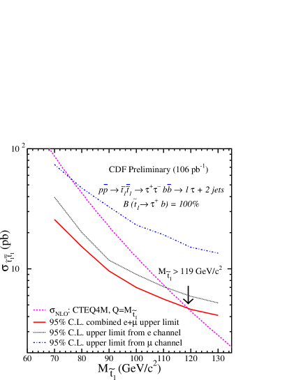
Figure 3: Limits in $\sigma_{\tilde{t}\overline{\tilde{t}}}$ in search for RPV m—sc SUGRA in decays of stop pair. We set the 95% C.L. mass limit of stop: $m_{\tilde{t}}>119\;{\rm GeV}$.

2.2 DØ search for resonant slepton in RPV mSUGRA

Resonant sleptons can be produced in the framework of RPV mSUGRA. With the assumption that $\lambda^{\prime}_{211}$ dominates, the production processes are shown in Figure 4. We search for signatures of resonant slepton in the final states which contain 2 muons and 2 jets. We apply the following cuts on $94\;{\rm pb^{-1}}$ of data:

• $E^{j}_{T}>20\;{\rm GeV\;(2\;jets)}$, $|\eta^{j}|<2.5$;

• $P^{\mu}_{T}>20\;{\rm Gev/c}$, $|\eta^{\mu_{1}}|,\;|\eta^{\mu_{2}}|<1.0,\;1.7$;

• $H_{T}\;({\rm all\;jets})>50\;{\rm GeV}$;

• cosmic ray rejection.

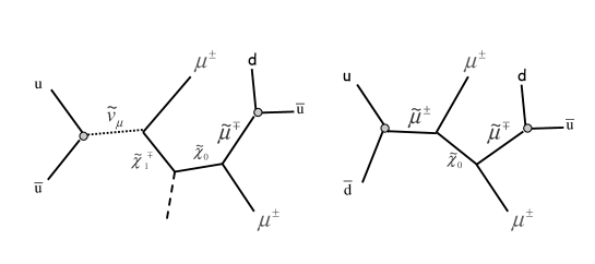
Figure 4: Feynman diagrams for resonant smuon and muon sneutrino production.

The major SM background events come from $Z+$ 2 jets, $t\overline{t}$ and $WW$ production. After the cuts above, the expected number of background events and the observed number of data events are listed in Table 2.

Table 2: Number of expected background events and the number of observed data events in search for resonant sleptons in the framework of RPV mSUGRA after all the analysis cuts are applied.

$Z+{\rm 2jets}$	$t\overline{t}$	$WW$	Total	Observed
4.8	0.53	0.01	$5.34\pm 0.07$	5

We use Neural Network to further increase the signal significance. The following seven variables are used in a three-layer Neural Network with a single node in the output layer: $E^{j_{1}}_{T}+E^{j_{2}}_{T}$, $P^{\mu_{1}}_{T}+P^{\mu_{2}}_{T}$, $M_{\mu_{1},\mu_{2}}$, $\Delta R_{\mu_{1},\mu_{2}}$ (separation of the two muons in $\eta-\phi$ plane, $\Delta R_{\mu_{1},j_{nn}}$ ($j_{nn}$ denotes the nearest-neighbor jet), sphericity, and aplanarity. The Neural Network output are shown in Figure 5. After applying the cuts indicated by the arrows in the plots, we expect $1.01\pm 0.02$ SM background events and observe 2 in the data. Limit contours in the $m_{1/2}-m_{0}$ plane for $\mu<2,\;\tan\beta=2$ is shown in Figure 6. Three coupling $\lambda^{\prime}_{211}$ strengths are shown. We are able to exclude $m_{1/2}$ up to 260 GeV for $\lambda^{\prime}_{211}=0.09$.

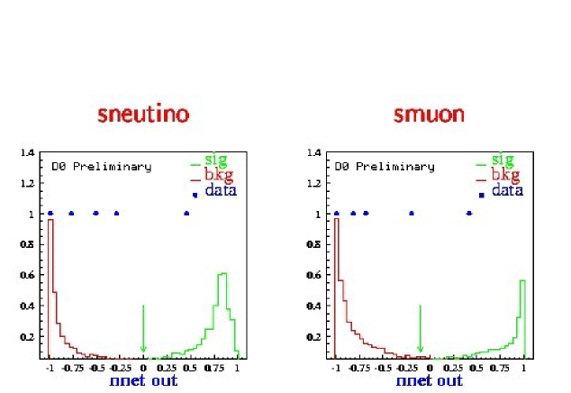
Figure 5: Neural Network output for signal (histograms peaked near 1), background (histograms peaked at -1), and data (points). The plot on the left is for the smuon channel, and the plots on the right is for the muon sneutrino channel.

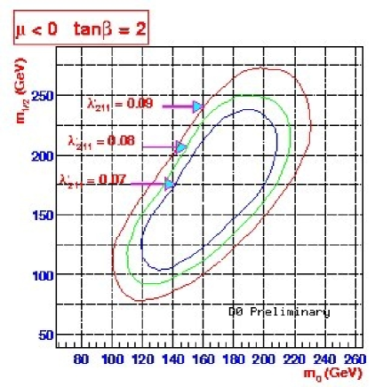
Figure 6: 95% C.L. limit contours in $m_{1/2}-m_{0}$ plane obtained in searching for resonant slepton in RPV mSUGRA. Three $\lambda^{\prime}_{211}$ coupling constants are shown assuming $\mu<0$ and $\tan\beta=2$.

2.3 DØ search for RPV mSUGRA in dimuon and four-jets channel[8]

In this analysis, we make the following assumptions:

• SUSY particles are pair produced;

• only one RPV coupling dominates, namely $\lambda^{\prime}_{222}$;

• only the LSP, assumed to be the lightest neutralino, $\widetilde{\chi}^{0}_{1}$, undergoes RPV decay.

The relevant Feynman diagram is shown in Figure 7. We apply the following cuts to enhance the signal significance in $77.5\;{\rm pb^{-1}}$ of data:

• $E^{j}_{T}>15\;{\rm GeV}$, $|\eta^{j}|<2.5$ (4 jets);

• $P^{\mu_{1}}_{T}>15\;{\rm GeV/c}$, $|\eta^{\mu_{1}}|<1.0$ and $P^{\mu_{2}}_{T}>10\;{\rm GeV/c}$, $|\eta^{\mu_{2}}|<1.7$, respectively;

• $H_{T}\;({\rm muons\;and\;jets})>150\;{\rm GeV}$;

• Aplanarity $>0.03$;

• $M_{\mu_{1},\mu_{2}}>5\;{\rm GeV}$.

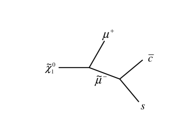
Figure 7: Feynman diagram of $\widetilde{\chi}^{0}_{1}$ decay and the subsequent RPV decay of smuon.

The major SM backgrounds are from $Z+{\rm jets}$ and $t\overline{t}$ processes. The expected number of these events surviving the cuts above are $0.14\pm 0.03$ for $Z+{\rm jets}$ and $0.04\pm 0.01$ for $t\overline{t}$, respectively. We observed 0 event in our data. The typical number of signal events are listed in Table 3. Since no signal is seen in our data, a 95% C.L. limit contour in $m_{1/2}$-$m_{0}$ plane are set and shown in Figure 8. For the case of $\tan\beta=2$, we exclude $m_{\tilde{q}}<240\;{\rm GeV}$ and $m_{\tilde{g}}<224\;{\rm GeV}$.

Table 3: Number of expected signal events after all the selection cuts for various representative signal parameters in search for RPV mSUGRA in dimuon and four jets channel.

$m_{0}$	$m_{1/2}$	${\rm N_{signal}}$
80	90	2.7
190	90	2.1
260	70	2.7
400	90	0.8

Figure 8: 95% C.L. limits in $m_{1/2}-m_{0}$ plane for $\tan\beta=2$ (plot on the left) and $\tan\beta=6$ (plot on the right) in search for RPV mSUGRA in dimuon and four-jets channel. We assumed that $\mu<0$ and $A_{0}=0$.

2.4 DØ search for RPC mSUGRA in single electron + $\geq 4$ jets + ${\hbox{$E$\kern-6.00006pt\lower-0.43057pt\hbox{/}}}_{T}$ channel[9]

DØ also conducted a search for $R_{p}$-conserving mSUGRA in a previous unexplored single electron channel. The search is particularly sensitive to the moderate $m_{0}$ region where charginos and neutralinos decay mostly into SM $W$ and/or $Z$ bosons which have large branching fractions to jets. One of the dominant process which produces our required final state is shown in Figure 9.

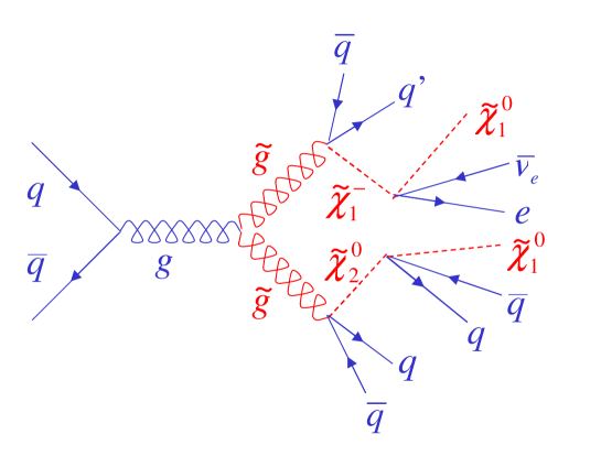
Figure 9: Feynman diagram for gluino pair production and decay to an electron, multijets, and produce ${\hbox{$E$\kern-6.00006pt\lower-0.43057pt\hbox{/}}}_{T}$. The three-body decays are in fact cascade decays in which off-shell particles or sparticles are produced. $R_{p}$ is assumed to be conserved.

The total amount of data used in this search is $92.7\;{\rm pb^{-1}}$. The data events are required to pass the following initial selections:

• one electron in the good fiducial volume ($|\eta^{e}_{\rm det}|<1.1$ or $1.5<|\eta^{e}_{\rm det}|<2.5$), and $E^{e}_{T}>20\;\rm{GeV}$, $|\eta^{e}|<2.0$;

• no extra electrons in the good fiducial volume with $E^{e}_{T}>15\;\rm{GeV}$;

• no isolated muons;

• $E_{T}^{j}>15\;\rm{GeV}$, $|\eta^{j}_{\rm det}|<2.5$ (4 jets);

• $\mbox{\mbox{${\hbox{$E$\kern-6.00006pt\lower-0.43057pt\hbox{/}}}_{T}$}}>25\;\rm{GeV}$.

The major SM backgrounds and fakes are from $t\overline{t}$, $WW$, $W+\geq 4{\rm jets}$, and multijet processes. After the initial selection cuts above, we observe 72 events in the data and expect $80\pm 10$ background events. The breakdown of background events in their respective type is shown in Table 4.

Table 4: Number of expected background events after initial selection cuts in search for $R_{p}$-conserving mSUGRA in the single electron + jets + ${\hbox{$E$\kern-6.00006pt\lower-0.43057pt\hbox{/}}}_{T}$ channel.

$t\overline{t}$	$WW$	$WW+\geq 4\;{\rm jets}$	Multijet	Total
$16.8\pm 5.2$	$1.4\pm 0.3$	$43.0\pm 7.6$	$19.1\pm 4.7$	$80\pm 10$

We use Neural Network to enhance the signal significance to set a strong limit. The input variables to the Neural Network are: $E^{j_{3}}_{T}$, $E^{e}_{T}$, ${\hbox{$E$\kern-6.00006pt\lower-0.43057pt\hbox{/}}}_{T}$, $H_{T}$ (all jets), $M_{T}$(e,${\hbox{$E$\kern-6.00006pt\lower-0.43057pt\hbox{/}}}_{T}$), aplanarity, $\Delta\phi_{e,\mbox{\mbox{${\hbox{$E$\kern-4.20004pt\lower-0.3014pt\hbox{/}}}_{T}$}}}$, $\cos\theta^{*}_{j}$, and $\cos\theta^{*}_{j}$, where $\theta^{*}_{j(e)}$ is the polar angle of the higher-energy jet (electron) from $W$ boson decay in the rest frame of the parent $W$ boson, relative to the direction of flight of the $W$ boson. This is calculated by fitting the events to the $t\overline{t}$ assumption. The distribution of these variables for signal, background, and data are shown in Figure 10. The signal in the plot is generated by SPYTHIA[10] with parameters: $m_{0}=170\;{\rm GeV}$, $m_{1/2}=58\;{\rm GeV}$, $\tan\beta=3$, $\mu<0$, and $A_{0}=0$. Both signal and background distributions are normalized to the total number of expected background events ($80\pm 10$). The distribution for the Neural Network output is shown in Figure 11. Shown in the insert of that figure is a plot of signal significance as a function of Neural Network output. We apply our final cut on Neural Network output at the highest signal significance. For the reference signal sample mentioned above, we cut at NNoutput = 0.825. We expect 10.4 signal events, 4.4 background events and observe 4 data events after this NNoutput cut.

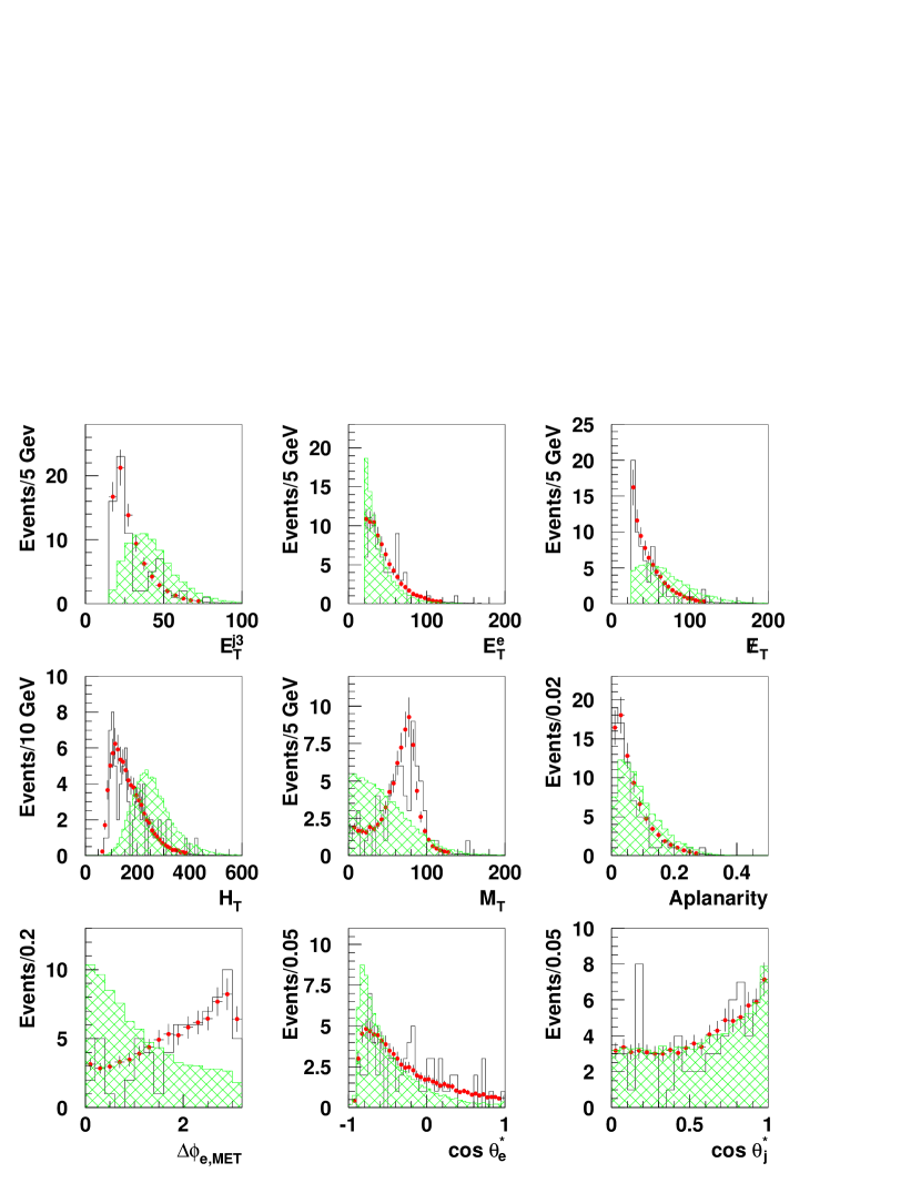
Figure 10: Distribution of Neural Network input variables for signal (hatched histogram), background (open histogram), and data (points) in search for $R_{p}$-conserving mSUGRA in single electron + $\geq 4$ jets + ${\hbox{$E$\kern-6.00006pt\lower-0.43057pt\hbox{/}}}_{T}$ channel. The signal and background histograms are normalized to the number of expected background events ($80\pm 10$). We observe $72$ events in our data.

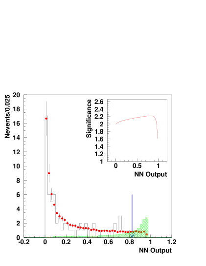
Figure 11: Distribution of Neural Network output for signal (hatched histogram), background (open histogram), and data (points) in search for $R_{p}$-conserving mSUGRA in single electron + $\geq 4$ jets + ${\hbox{$E$\kern-6.00006pt\lower-0.43057pt\hbox{/}}}_{T}$ channel. All histograms are normalized to their respective total number of events. The insert shows a signal significance as function of Neural Network output. The arrow indicates where the signal significance is the highest and where we apply our final cut. We retain events to the right of the arrow. For this reference signal sample, which is generated with $m_{0}=170\;{\rm GeV}$, $m_{1/2}=58\;{\rm GeV}$, $\tan\beta=3$, $\mu<0$, and $A_{0}=0$, $10.4$ signal events and $4.4$ background events are expected to survive the final cut. We observe $4$ in the data.

Since no signal is observed in our data, a limit is set. The limit contour is presented in $m_{1/2}-m_{0}$ plane for $\tan\beta=3$, $\mu<0$, and $A_{0}=0$ in Figure 12. It extends the limit set by LEP I and a previous DØ search in the dilepton channel in the moderate $m_{0}$ region. The current best limit is set by LEP[11] and the best Tevatron limit is set by the CDF collaboration[12].

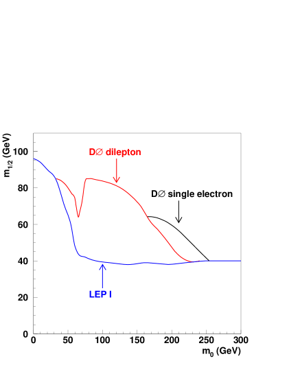
Figure 12: 95% limit contour in $m_{1/2}-m_{0}$ plane in search for $R_{p}$-conserving mSUGRA in single electron + $\geq 4$ jets + ${\hbox{$E$\kern-6.00006pt\lower-0.43057pt\hbox{/}}}_{T}$ channel with $\tan\beta=3$, $\mu<0$, and $A_{0}=0$. Also shown in the plot are limits from LEP I and a previous DØ search in the dilepton channel.

3 Search for Large Extra Dimension

A theory of Large Extra Dimensions (LED) has recently been proposed to solve the hierarchy problem[13]. It is argued that gravity lives in $n$ additional large spatial dimensions while the all the fields of SM are constrained to a three-dimensional brane which corresponds to our four space-time dimension. The usually weak gravitational interactions in the three-brane is in fact strong in the $n$ additional dimensions at an effective Planck Scale $M_{D}$, which is near the weak scale. Gauss’ Law then relates $M_{D}$ with $n$ and the Planck scale, $M_{pl}$ as:

$$M_{pl}=8\pi R^{n}M^{n+2}_{D},$$ (2)

where $R$ is the radius of the compactified space in which the gravitational interaction is strong.

While there are many interesting models to solve the hierarchy problem in the framework of large extra dimension, we will focus on the one proposed by Arkani-Hamed, Dimopoulos, and Dvali[13], in the GRW[14] convention. One interesting testable aspect of this theory is that it predicts the existence of Kaluza Klein (KK) tower of massive gravitons which can interact with the SM fields on the three-brane. We report two searches for LED:

• virtual graviton exchange in diphoton production (CDF);

• direct graviton production in $q\overline{q}\rightarrow gG$ (DØ).

3.1 CDF search for LED in diphoton events

The differential cross section of diphoton production at the hadron collider can be written in Eq. (3):

$$\frac{d\sigma}{dM_{\gamma\gamma}}=\frac{d\sigma}{dM_{\gamma\gamma}}\Bigg{|}_{SM}+\eta\frac{d\sigma}{dM_{\gamma\gamma}}\Bigg{|}_{int}+\eta^{2}\frac{d\sigma}{dM_{\gamma\gamma}}\Bigg{|}_{KK},$$ (3)

where $\eta=\frac{\lambda}{M_{D}}$, and $\lambda$ is of order 1. The three terms in Eq. (3) are contributions from the SM alone, interference of SM and LED, and LED itself, respectively. Our selection requirements are:

• $E^{\gamma}_{T}>22\;{\rm GeV}$ and $|\eta^{\gamma}_{det}|<1.0$ for central-central (CC) [1] diphoton events;

• $E^{\gamma_{c}}_{T}>25\;{\rm GeV}$, $|\eta^{\gamma_{c}}_{det}|<1.0$ and $E^{\gamma_{p}}_{T}>22\;{\rm GeV}$, $1.1<|\eta^{\gamma_{p}}_{det}|<2.4$ for central-plug (CP)[1] diphoton events.

After these selections we expect that in the $100\;{\rm pb^{-1}}$ of data we use for this analysis, there are $96\pm 31$ SM events and $184\pm 63$ fake events in CC and $76\pm 31$ SM events and $132\pm 28$ fake events in EC. We observe 287 and 192 events, respectively. Since no excess is seen in our data, we perform a log-likelihood fit on the diphoton invariant mass spectrum to Eq. (3) to extract the 95% C.L. limit on $M_{D}$. The diphoton invariant mass spectra of data, background, and signal are shown in Figure 13. From the fit, we obtain $M_{D}>1.01\;{\rm TeV}$. Note that DØ performed a similar search which included dielectron events in the data set ($127\;{\rm pb^{-1}}$). In addition to invariant mass, the polar angle of the electron or photon in the rest frame of the dielectron or diphoton system was also used as a parameter in the fit. The extracted limit is $M_{D}>1.21\;{\rm TeV}$[15].

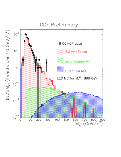
Figure 13: Invariant mass spectrum of diphoton events for SM+Fakes, direct LED contribution, the LED/SM interference, and data in search for LED in the photon + ${\hbox{$E$\kern-6.00006pt\lower-0.43057pt\hbox{/}}}_{T}$ channel.

3.2 DØ search for direct graviton production in LED in the monojet channel

Graviton in LED can also be produced at the Tevatron directly through $q\overline{q}\rightarrow gG$ and $gg\rightarrow gG$. The distinct signature in the detector is a single jet (monojet) with large missing transverse energy.

In this DØ search, the signal events are generated using a subroutine written by Lykken and Matchev[16] as the external process to PYTHIA[17]. To reduce the backgrounds, which are dominated by $Z\rightarrow\nu\nu$ and $W(l\nu)$ fake events, DØ require that $E^{j}_{T}>150\;{\rm GeV}$, $|\eta^{j}_{det}|<1.0$, and $\mbox{\mbox{${\hbox{$E$\kern-6.00006pt\lower-0.43057pt\hbox{/}}}_{T}$}}>150\;{\rm GeV}$. We also reject events with isolated muons or with $E^{j_{2}}_{T}>50\;{\rm GeV}$, where $j_{2}$ denotes the second leading jet in $E_{T}$ in the event. The total amount of data used in this analysis is $78.8\;{\rm pb^{-1}}$. After applying the cuts mentioned above, we observe 38 event and expect $30.2\pm 4.0$ $WZ$ SM events and $7.8\pm 7.1$ multijet and cosmic fake events. The ${\hbox{$E$\kern-6.00006pt\lower-0.43057pt\hbox{/}}}_{T}$ spectrum after the cuts is shown in Figure 14. The expected total background agrees with data very well. We thus set the 95% C.L. limits on $M_{D}$ as shown in Figure 15. Also plotted in the figure are limits obtained by LEP experiments. We note that at higher extra dimensions $n\geq 5$, because the large center-of-mass energy the Tevatron can reach, DØ limit extends those obtained by the LEP experiments. The numeric value of the limit at each extra dimension is also listed in Table 5.

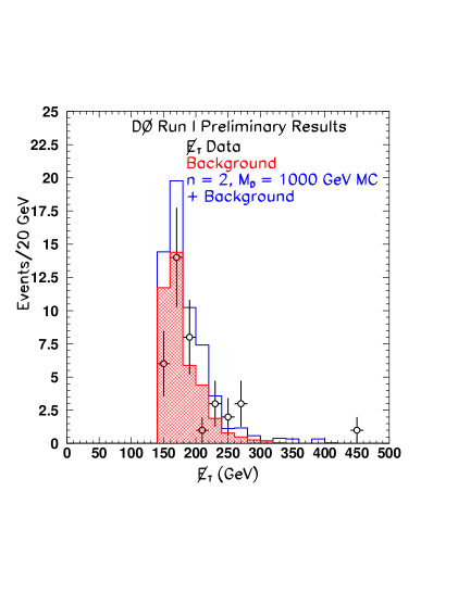
Figure 14: ${\hbox{$E$\kern-6.00006pt\lower-0.43057pt\hbox{/}}}_{T}$ spectrum for background (hatched histogram), expected signal for $n=2$ and $M_{D}=1000\;{\rm GeV}$ (stacked open histogram), and data (points) in search for LED in the monojet channel. The data and background agree very well.

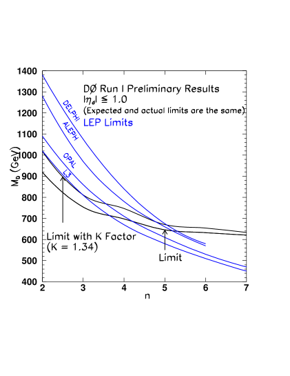
Figure 15: 95% C.L. lower limits on $M_{D}$ in the DØ search for LED in the monojet channel. Limits with and without k-factor ($k=1.34$) are plotted. Also shown is the limits obtained by the LEP experiments.

Table 5: 95% C.L lower limits on the effective Planck scale $M_{D}$ as a function of number of extra dimension $n$ obtained by DØ search for LED in monojet channel. No k-factor is applied.

$n$	2	3	4	5	6	7
$M_{D}$ (TeV)	0.89	0.73	0.68	0.64	0.63	0.62

4 Search for leptoquarks in jets + ${\hbox{$E$\kern-6.00006pt\lower-0.43057pt\hbox{/}}}_{T}$ channel[18]

Because of the flavor symmetry between the lepton and quark sectors of the SM, theories have been developed to explore the possible direct couplings between the leptons and the quarks through new particles. Leptoquarks (LQ) are one of these postulated particles. They are either scalar[19] or vector[20] bosons which carry both color and fractional electric charge. At the Tevatron, LQ can be pair produced through strong interaction: $p\overline{p}\rightarrow LQ\overline{LQ}+X$.

Limits from flavor-changing neutral currents imply that leptoquarks of low mass ${\cal O}$(TeV) couple only within a single generation[21]. Leptoquark pair can decay into $l^{\pm}l^{\mp}q\overline{q}$, $l^{\pm}\nu q\overline{q}$, and $\nu\overline{\nu}q\overline{q}$ final states. Both CDF and DØ have performed search in the dilepton and single lepton channels. The analysis reported here is based on the $\nu\overline{\nu}q\overline{q}$ final state. It is sensitive to leptoquarks of all three generations. Searches for both scalar and vector leptoquarks are performed. In the case of vector leptoquark, we consider specific cases of couplings resulting in the minimal cross section ($\sigma_{\rm min}$), Minimal Vector coupling (MV), and Yang-Mills coupling (YM)[22].

The total amount of data used in this analysis is $85.2\;{\rm pb^{-1}}$. The following initial cuts are applied:

• $E^{j_{1}}_{T}>50\;{\rm GeV}$, $E^{j_{2}}_{T}>40\;{\rm GeV}$, and at least one of the jets is in $|\eta|<1.0$;

• $\mbox{\mbox{${\hbox{$E$\kern-6.00006pt\lower-0.43057pt\hbox{/}}}_{T}$}}>40\;{\rm GeV}$;

• $\Delta\phi({\rm all\;jets,\mbox{${\hbox{$E$\kern-6.00006pt\lower-0.43057pt\hbox{/}}}_{T}$}})>30^{\circ}$, $\Delta\phi(j_{2},\mbox{\mbox{${\hbox{$E$\kern-6.00006pt\lower-0.43057pt\hbox{/}}}_{T}$}})>60^{\circ}$.

Events with isolated muons are rejected. After the initial cuts, we are left with 231 events in the data. The major SM background and fakes come from multijet, $W+$ jets, $Z+$ jets, and $t\overline{t}$ processes. We estimate that there are $242\pm 19({\rm stat})^{+29}_{-10}({\rm sys})$ of such events in the data after the initial cuts. The data and background estimation agree very well.

Figure 16: Neural Network output for scalar (plot on the left) and vector (plot on the right) leptoquark signals. The points are data and the histograms are the expected background. We apply the final cut at the Neural Network output values indicated as arrows in the plots to obtain a strong limit.

In order to set a strong limit, we use Neural Network to enhance the signal significance. The input variables are ${\hbox{$E$\kern-6.00006pt\lower-0.43057pt\hbox{/}}}_{T}$ and $\Delta\phi(j_{1},j_{2})$ for the scalar leptoquark signal, and ${\hbox{$E$\kern-6.00006pt\lower-0.43057pt\hbox{/}}}_{T}$ and $E^{j_{2}}_{T}$ for the vector leptoquark signal. The distribution of the Neural Network output is shown in Figure 16. We calculate a signal significance as a function of Neural Network output. The values which correspond to the maximal signal significance are indicated as arrows in Figure 16. After removing events to the left of the arrows, we are left with $56\pm 3$ ($13\pm 3$) expected background events and 58 (10) observed data events in the case of scalar (vector) leptoquark signal. The resulting 95% C.L. limit contours are shown in Figure 17. From the limit contours we obtain the 95% C.L. limit on the leptoquark masses: $M_{SLQ}>98\;{\rm GeV}$, and $M_{VLQ}>200,238,298\;{\rm GeV}$ for $\sigma_{min}$, MV, and YM coupling, respectively. The results of this analysis are also combined with those obtained in the previous first and second generation leptoquark searches by DØ[24, 25]. The resulting mass limits as a function of BR(${\rm LQ}\rightarrow l^{\pm}q$) are shown in Figure 18. The gaps at small BR in the previous analyses are filled as a result of this investigation.

Figure 17: 95% C.L. limit on leptoquark production cross section as a function of leptoquark mass for the scalar (plot on the left) and vector (plot on the right) leptoquarks. The dotted curves are theoretical calculations and the 95% confidence limit set by a previous DØ search [23] using one tenth the amount of the data as what are in this analysis.

Figure 18: Combined 95% C.L. limit on scalar (plot on the left) and vector (plot on the right) leptoquark mass as a function of leptoquark branch fraction into lepton and quark: BR(${\rm LQ}\rightarrow l^{\pm}q$). The results combined are those from this analysis, and those from previous DØ searches for the first and second generation leptoquarks.

5 Model Independent Searches

During the past year, both CDF and DØ performed searches that are mostly based on final states of data rather than specific models that result in those final states. Understanding the final states makes the search of models a much more straightforward process.

5.1 CDF photon + ${\hbox{$E$\kern-6.00006pt\lower-0.43057pt\hbox{/}}}_{T}$ analysis[26]

Photon + ${\hbox{$E$\kern-6.00006pt\lower-0.43057pt\hbox{/}}}_{T}$ is an interesting signal for many new physics. In this analysis, we first prepare a set of photon + ${\hbox{$E$\kern-6.00006pt\lower-0.43057pt\hbox{/}}}_{T}$ data sample with all the contributions from SM background and fakes understood. We then look at models which may result in the photon + ${\hbox{$E$\kern-6.00006pt\lower-0.43057pt\hbox{/}}}_{T}$ final state. We apply the following selection cuts to reduce the data to a reasonable size:

• $E^{\gamma}_{T}>55\;{\rm GeV}$ and $|\eta^{\gamma}_{det}|<1.0$;

• $\mbox{\mbox{${\hbox{$E$\kern-6.00006pt\lower-0.43057pt\hbox{/}}}_{T}$}}>45\;{\rm GeV}$;

• no jets with $E^{j}_{T}>15\;{\rm GeV}$ or tracks with $P_{T}>5\;{\rm GeV/c}$.

We observe 11 events and expect 11 background events in $87\;{\rm pb^{-1}}$ of data. The background sources and their expected number of events surviving the cuts are listed in Table 6.

Table 6: SM background sources and their expected number of events in $87\;{\rm pb^{-1}}$ of photon + ${\hbox{$E$\kern-6.00006pt\lower-0.43057pt\hbox{/}}}_{T}$ data.

Background source	Events
cosmic rays	$6.3\pm 2.0$
$Z\gamma\rightarrow\nu\nu\gamma$	$3.2\pm 1.0$
$W\rightarrow e\nu$	$0.9\pm 0.1$
prompt diphoton	$0.4\pm 0.1$
$W\gamma$	$0.3\pm 0.1$
Total	$11.0\pm 2.2$

Since no signal is seen in our data, these 11 events can be used to exclude models or to set limits on models. In order to do that, a generic detector acceptance and efficiency for photons has to be measured. They are shown in Figure 19. We can then convolute photon + ${\hbox{$E$\kern-6.00006pt\lower-0.43057pt\hbox{/}}}_{T}$ events from any model with the acceptance, efficiency, and detector resolution, to calculate the total event acceptance for the model.

Figure 19: Detector acceptance and detection efficiency of photons at CDF.

We look into two models. The first one is a superlight gravitino[27] model in which the only supersymmetric particle light enough to be produced at Tevatron is the gravitino $\widetilde{G}$. The process is $q\overline{q}\rightarrow\widetilde{G}\widetilde{G}\gamma$, in which the photon comes from initial state radiation and serves as a tagger for the process. The SUSY-breaking scale $F$ can be related to the mass of the gravitino $m_{3/2}$ by $F=\sqrt{3}m_{3/2}M_{pl}$, where $M_{pl}\approx 2.4\times 10^{18}$ is the Planck scale. By convoluting the model through our Monte Carlo and acceptance, efficiency, and resolution functions, we obtain a new 95% C.L. limit of $\sqrt{F}>221\;{\rm GeV}$, or $m_{3/2}>1.17\times 10^{-5}\;{\rm eV}$.

The second model we look into is large extra dimension (LED) in the framework of Arkani-Hamed, Dimopoulos, and Dvali[13]. The relevant process is $q\overline{q}\rightarrow G_{kk}\gamma$. We list the calculated 95% C.L. limit on the effective Planck scale $M_{D}$ in the GRW[14] convention in Table 7. Also listed in the table is the best results obtained by the LEP experiments. As in the monojet case, the CDF limit extends that from the LEP at higher extra dimension due to the higher center-of-mass energy of the Tevatron.

Table 7: Lower limits in the effective Planck scale $M_{D}$ as a function of number of extra dimension $n$ obtained by CDF search for LED in photon + ${\hbox{$E$\kern-6.00006pt\lower-0.43057pt\hbox{/}}}_{T}$ channel.

$n$	4	6	8
$M_{D}$ (GeV)	549	581	602
$M_{D}$ (GeV) (LEP)	680[29]	510[29]	411[30]

5.2 Quaero – automatic data analysis machine at DØ[31]

Quaero, which means “to seek” in Latin, uses DØ data which are publically available on the internet and automatically optimizes searches for any signal provided by the user. The data sets are categorized according to their final states. The backgrounds and their respective fractions have been calculated and are available to the user. It is understood that the data are well explained by the expected background and that the goal of the analysis is to set $\sigma^{95\%}$, the 95% C.L. upper limit, on the cross section of the model. At the Quaero web page, http://quaero.fnal.gov, users can use PYTHIA[17] to generate their model events which results in one of the available final states. They can then define a variable set $\vec{x}$ to be used to optimize the search. The optimization algorithm has the following steps:

• Kernel density estimation[32] is used to obtain a signal and background probability distribution $p(\vec{x}|s)$ and $p(\vec{x}|b)$, respectively;

• A discriminant function is defined as[32]:

  $$D(\vec{x})=\frac{p(\vec{x}|s)}{p(\vec{x}|s)+p(\vec{x}|b)};$$

• The sensitivity $S$ is defined as the reciprocal of $\overline{\sigma^{95\%}}$, which is the 95% C.L. limit on model cross section as a function of $D_{cut}$ on $D(\vec{x})$. An optimal $D_{cut}$ on $D(\vec{x})$ is chosen to minimize $\overline{\sigma^{95\%}}$, thus maximize $S$;

• The region of variable space having $D(\vec{x})>D_{cut}$ is used to determine the actual 95% C.L. cross section upper limit $\sigma^{95\%}$.

Based on Run 1 data, Quaero has set $\sigma^{95\%}$ for various models, including SM higgs production: $h\rightarrow WW\rightarrow e\mbox{\mbox{${\hbox{$E$\kern-6.00006pt\lower-0.43057pt\hbox{/}}}_{T}$}}2j$, $h\rightarrow ZZ\rightarrow ee2j$, $Wh\rightarrow e\mbox{\mbox{${\hbox{$E$\kern-6.00006pt\lower-0.43057pt\hbox{/}}}_{T}$}}2j$, and $Zh\rightarrow ee2j$; $W^{\prime}$ and $Z^{\prime}$ production: $W^{\prime}\rightarrow WZ\rightarrow e\mbox{\mbox{${\hbox{$E$\kern-6.00006pt\lower-0.43057pt\hbox{/}}}_{T}$}}2j$, $Z^{\prime}\rightarrow t\overline{t}\rightarrow e\mbox{\mbox{${\hbox{$E$\kern-6.00006pt\lower-0.43057pt\hbox{/}}}_{T}$}}4j$; and leptoquark production: $LQ\overline{LQ}\rightarrow ee2j$.

6 Conclusion

We have presented in this paper nine analyses which were finalized in year 2001. Even though we did not observe any signature of new physics, we are able to set stronger limits on them. New tools and techniques have been developed to equip us for more challenging searches. With more powerful detectors for both CDF and DØ, and an order of magnitude of increase in luminosity for expected for Run 2, we are looking forward to more exciting searches and possibly discoveries.

7 Acknowledgment

The author is thankful to both CDF and DØ Collaborations for the opportunity to present these new results at La Thuile 2002’. In particular the author would like to thank the following persons who actually carried out the analyses and provided the detail information: Abdelouahab Abdesselam, Sudeshna Banerjee, and Hai Zheng of the DØ Collaboration, and David Gerdes, Chris Hays, Teruki Kamon, Minjeong Kim, Bruce Knuteson, Yoshiyuki Miyazaki, Simona Murgia, Peter Onyisi, and Masashi Tanaka of the CDF Collaboration.

References

- 1 . CDF Collaboration, F. Abe et al., Nucl. Instr. Methods Phys. Res. A 271, 387 (1988).
- 2 . DØ Collaboration, S. Abachi et al., Nucl. Instr. Methods Phys. Res. A 338, 185 (1994).
- 3 . For reviews see P. Nath, R. Arnowitt, and A. H. Chamseddine, “Applied Supergravity” (World Scientific, Singapore, 1984); H. P. Nilles, Phys. Rept. 110, 1 (1984).
- 4 . D. V. Volkov and V. P. Akulov, Phys. Rev. Lett. 46B, 109 (1973); J. Wess and B. Zumino, Nucl. Phys. B70, 39 (1974).
- 5 . G. R. Farrar and P. Fayet, Phys. Lett. B 76, 575 (1978).
- 6 . For a review, see e.g., H. Haber and G. Kane, Phys. Rept. 117, 75 (1985).
- 7 . ALEPH Collaboration, hep-ex/0011008.
- 8 . DØ Collaboration, V. M. Abazov et al., hep-ex/0111053.
- 9 . DØ Collaboration, V. M. Abazov et al., hep-ex/0205002.
- 10 . S. Mrenna, hep-ph/9609360.
- 11 . LEP2 SUSY Working Group, http://www.cern.ch/LEPSUSY.
- 12 . CDF Collaboration, T. Affolder et al., Phys. Rev. Lett. 88, 041801 (2002).
- 13 . N. Arkani-Hamed, S. Dimopoulos, and G. Dvali, Phys. Lett. B 429, 263 (1998).
- 14 . G. F. Giudice, R. Rattazzi, and J. D. Wells, Nucl. Phys. B 544, 3 (1999).
- 15 . DØ Collaboration, B. Abbott et al., Phys. Rev. Lett. 86, 1156 (2001).
- 16 . J. Lykken and C. Matchev, private code.
- 17 . M. Bengtsson and T. Sjöstrand, Comp. Phys. Comm. 43, 367 (1987).
- 18 . DØ Collaboration, V. M. Abazov et al., Phys. Rev. Lett. 88, 191801 (2002).
- 19 . P. H. Frampton, Mod. Phys. Lett. A 7, 559 (1992).
- 20 . H. Georgi and S. Glashow, Phys. Rev. Lett. 32, 438 (1974); J .C .Pati and A. Salam, Phys. Rev. D 10, 275 (1974).
- 21 . H. U. Bengtsson, W. S. Hou, A. Soni, and D. H. Stork, Phys. Rev. Lett. 55, 2762 (1985).
- 22 . J. Blümlein, E. Boos, and A. Kryukov, Z. Phys. C 76, 137 (1997).
- 23 . DØ Collaboration, B. Abbott et al., Phys. Rev. Lett. 80, 2051 (1998); DØ Collaboration, V. M. Abazov et al., hex-ex/0105072.
- 24 . DØ Collaboration, V. M. Abazov et al., Phys. Rev. D 64, 092004 (2001).
- 25 . DØ Collaboration, B. Abbott et al., Phys. Rev. Lett. 83, 2896 (1999); DØ Collaboration, B. Abbott et al., Phys. Rev. Lett. 84, 2088 (2000).
- 26 . CDF Collaboration, D. Acosta et al., hep-ex/0205057.
- 27 . A. Brignole, F. Feruglio, M. L. Mangano, and F. Zwirner, Nucl. Phys. B 526, 136 (1998); erratum-ibid. B 582, 759 (2000).
- 28 . CDF Collaboration, T. Affolder et al., Phys. Rev. Lett. 85, 1378 (2000).
- 29 . P. Abreu et al., Eur. Phys. J. C 17, 53 (2000).
- 30 . M. Acciarri et al., Phys. Lett. B 470, 268 (1999).
- 31 . DØ Collaboration, B. Abbott et al., Phys. Rev. Lett. 87, 231801 (2001); http://quaero.fnal.gov/quaero/ .
- 32 . L. Holmstrom, S. Sain, and H. Miettinen, Comp. Phys. Commun. 88, 195 (1995).