Support Vector Machines in Analysis of Top Quark Production

Abstract

Multivariate data analysis techniques have the potential to improve physics analyses in many ways. The common classification problem of signal/background discrimination is one example. A comparison of a conventional method and a Support Vector Machine algorithm is presented here for the case of identifying top quark signal events in the dilepton decay channel amidst a large number of background events.

1 INTRODUCTION

A common problem in high energy physics is that of classification. Is it a signal or background event? Does the energy deposit correspond to a tau particle or not? There are many problems for which no explicit method exists to determine the correct output from the input data. One approach is to devise an algorithm which finds and exploits complex patterns in input/output examples (labeled training data) to learn the solution to the problem. This is called “supervised learning”. Such an algorithm can map each training example onto two categories (“binary classification”), more than two categories (“multi-class classification”), or continuous, real-valued output (“regression”).

One possible goal is to modify the learning algorithm in an iterative procedure until all training data are classified correctly (i.e. no mistakes). A potential problem with this goal is noisy training data. There may be no correct underlying classification function. Two similar training examples may be in different categories. An example is distinguishing a photon deposit in a calorimeter from a $\pi^{o}\rightarrow\gamma\gamma$ deposit. Another problem may be that the resulting algorithm misclassifies unseen data because it has “overfit” the training data. A better goal is to optimize “generalization” – the ability to correctly classify unseen data. In this approach we should not add extra complexity unless it causes a significant improvement in performance. Potential problems include making mistakes due to local minima, overfitting when using a complex mapping function on a small training set, and having a large number of tunable parameters which makes the algorithm difficult to use.

Section 2 of this paper shows how the Support Vector Machine learning methodology addresses these problems. The description closely follows that of several references in the literature [1, 2, 3]. The use of hyperplane classifiers in SVMs is described first for the linear, separable case. This is followed by the extension to nonlinear SVMs and to nonseparable data. In section 3, the results of a study using SVMs in an analysis of top quark production are presented.

2 SUPPORT VECTOR MACHINE METHODOLOGY

2.1 Overview

In the early 1960s the support vector method was developed to construct separating hyperplanes for pattern recognition problems [4, 5]. In the 1990s it was generalized for constructing nonlinear separating functions [6, 7] and for estimating real-valued functions (regression) [8]. Current activities [9] include a special SVM issue of the journal Neurocomputing (2002), a NATO Advanced Study Institute on Learning Theory and Practice (July, 2002), an International Workshop on Practical Application of Support Vector Machines in Pattern Recognition (August, 2002), and a Special Session on Support Vector Machines at the International Conference on Neural Information Processing (November, 2002).

Applications of SVMs include text categorization, character recognition, bioinformatics and face detection. The main idea of the SVM approach is to map the training data into a high dimensional feature space in which a decision boundary is determined by constructing the optimal separating hyperplane. Computations in the feature space are avoided by using a kernel function. This approach uses concepts from statistical learning theory to describe which factors have to be controlled for good generalization.

2.2 Generalization and Capacity

The formal goal is to estimate the function $f:\Re^{N}\rightarrow\{\pm 1\}$ using input/output training data

$(\vec{x}_{1},y_{1}),...,(\vec{x}_{\ell},y_{\ell})\in\Re^{N}\times\{\pm 1\}$

such that $f$ will correctly classify unseen examples $(\vec{x},y)$, i.e. $f(\vec{x})=y$. $\ell$ is the number of training examples. There is a tension between the function’s complexity and the resulting accuracy. According to statistical learning theory, for good generalization we should restrict the class of functions from which $f$ is chosen. Simply minimizing the training error,

$(1/\ell)\sum_{i}\mid f(\vec{x}_{i})-y_{i}\mid$,

does not necessarily result in good generalization. More precisely, we restrict the class of functions to one with a “capacity” suitable for the amount of available training data. The “capacity” is the richness or flexibility of the function class. Low capacity leads to good generalization, regardless of the dimensionality of the space, assuming the function describes the data well. Controlling the capacity is one way to improve generalization accuracy.

2.3 Hyperplane Classifiers

Support Vector classifiers are based on the class of hyperplanes

$(\vec{w}\cdot\vec{x})+b=0$

with $\vec{w}\in\Re^{N},$ $b\in\Re$ and corresponding to the decision function

$f(\vec{x})=$ sign$[(\vec{w}\cdot\vec{x})+b]$.

$\vec{w}$ is called the “weight vector” and b the “threshold”. $\vec{w}$ and b are the parameters controlling the function and must be learned from the data. For pedagogical purposes we are considering first the linear, separable, binary classification case, i.e. $f(\vec{x})$ is a linear function of $\vec{x}$ and there are two classes which can be separated completely.

The unique hyperplane with maximal margin of separation between the two classes is called the optimal hyperplane. It can be shown that it has the lowest capacity of any hyperplane, which minimizes the risk of overfitting. The optimization problem thus becomes one of finding the optimal hyperplane. This is different than the “intuitive” way of decreasing capacity by reducing the number of degrees of freedom (e.g. decreasing the number of nodes or layers in a neural network). A geometric interpretation is that the hyperplane splits the input space into two parts, each one corresponding to a different class. Figure 1a shows a two dimensional example with two classes denoted by solid circles ($y_{i}=+1$) and open circles ($y_{i}=-1$). The optimal hyperplane is shown by the solid line between the two classes.

Figure 1: (a) Geometric interpretation of hyperplane classifier in two dimensions. (b) Cartoon showing how a nonlinear problem in input space is mapped onto a linear problem in feature space.

The size of the margin is inversely proportional to the norm of $\vec{w}$. To find the optimal hyperplane, $\|\vec{w}\|^{2}$ must be minimized subject to constraints $y_{i}[(\vec{w}\cdot\vec{x}_{i})+b]\geq 1$ for $i=1,...\ell$. The $\vec{x}_{i}$ for which the equality holds are called “support vectors”. They carry all information about the problem. They lie on a hyperplane defining the margin and their removal would change the solution. In Figure 1a $\vec{x}_{1}$ and $\vec{x}_{2}$ are examples of support vectors.

To solve this constrained quadratic optimization problem, we first reformulate it in terms of a Lagrangian,

$\mathcal{L}(\vec{w},b,\alpha_{i})=(1/2)\|\vec{w}\|^{2}-\sum_{i}\alpha_{i}[y_{i}((\vec{x}_{i}\cdot\vec{w})+b)-1]$.

This reformulation is done because it is easier to handle constraints on the Lagrange multipliers, $\alpha_{i}$ ($\alpha_{i}\geq 0$), and the training data will only appear in the form of dot products between vectors. This will allow us to generalize to the nonlinear case. Note that the number of free parameters in an SVM increases as the number of training examples increases.

Generalization theory indicates how to control the capacity by controlling the margin of separation. Specifically, we need to find the optimal hyperplane. Optimization theory provides mathematical tools to find this hyperplane. We need to minimize $\mathcal{L}$ with respect to $\vec{w}$ and b (primal variables) and maximize $\mathcal{L}$ with respect to $\alpha_{i}$ (dual variables). The solution has an expansion in terms of a subset of input vectors (with $\alpha_{i}\neq 0$) called Support Vectors,

$\vec{w}=\sum_{i}\alpha_{i}y_{i}\vec{x}_{i}$.

$\alpha_{i}$ corresponds to the difficulty in classifying the point. Small $\alpha_{i}$ means easy classification. In dual form the optimization problem becomes one of finding the $\alpha_{i}$ which maximize

$\mathcal{L}=\sum_{i}\alpha_{i}-(1/2)\sum_{i,j}\alpha_{i}\alpha_{j}y_{i}y_{j}\vec{x}_{i}\cdot\vec{x}_{j}$

subject to the constraints $\alpha_{i}\geq 0$ and $\sum_{i}\alpha_{i}y_{i}=0$. The decision function is

$f(\vec{x})=$ sign$[\sum_{i}y_{i}\alpha_{i}(\vec{x}\cdot\vec{x}_{i})+b]$

Both the optimization problem and the final decision function depend only on dot products between input vectors. This is crucial for the successful generalization to the nonlinear case.

2.4 Feature Spaces and Kernels

If $f(\vec{x})$ is a nonlinear function of $\vec{x}$ one possible approach is to use a neural network, which consists of a network of simple linear classifiers. Problems with this approach include many parameters and the existence of local minima. The SVM approach is to map the input data into a high, possibly infinite dimensional feature space, $\mathcal{F}$, via a nonlinear map $\Phi:R^{N}\rightarrow\mathcal{F}$. Then the optimal hyperplane algorithm can be used in $\mathcal{F}$ (see Figure 1b). This high dimensionality may lead to a practical computational problem in feature space. Since the input vectors appear in the problem only inside dot products, however, we only need to use dot products in feature space. If we can find a kernel function, $\mathcal{K}$, such that

$\mathcal{K}(\vec{x}_{1},\vec{x}_{2})=\Phi(\vec{x}_{1})\cdot\Phi(\vec{x}_{2})$

then we don’t need to know $\Phi$ explicitly. Mercer’s Theorem tells us that a function $\mathcal{K}(\vec{x},\vec{y})$ is a kernel, i.e. there exists a mapping $\Phi$ such that

$$\mathcal{K}(\vec{x}_{1},\vec{x}_{2})=\Phi(\vec{x}_{1})\cdot\Phi(\vec{x}_{2})$$

if

$$\int\mathcal{K}(\vec{x},\vec{y})g(\vec{x})g(\vec{y})d\vec{x}d\vec{y}\geq 0$$

for all g such that $\displaystyle\int g(\vec{x})^{2}d\vec{x}$ is finite. Mercer’s Theorem does not tell us how to construct $\Phi$ but this explicit mapping is not needed to solve the problem. Rather than creating a function and testing whether it is a kernel function, we can choose from known kernel functions:

• $\mathcal{K}(\vec{x},\vec{y})=(\vec{x}\cdot\vec{y})^{d}$
  (polynomial of degree d)

• $\mathcal{K}(\vec{x},\vec{y})=$ exp$(-\parallel{\vec{x}-\vec{y}}\parallel^{2}/(2\sigma^{2}))$
  (Gaussian Radial Basis Function)

• $\mathcal{K}(\vec{x},\vec{y})=$ tanh$(\kappa(\vec{x}\cdot\vec{y})+\theta)$
  (sigmoid)

Different kernel functions lead to similar classification accuracies and Support Vector sets.

2.5 Nonlinear SVMs

To extend the methodology described above to nonlinear problems, we substitute $\Phi(\vec{x}_{i})$ for each training example $\vec{x}_{i}$ and substitute the kernel for dot products of $\Phi$. The decision function then becomes

$f(\vec{x})=$ sign$[\sum_{i}y_{i}\alpha_{i}\mathcal{K}(\vec{x},\vec{x}_{i})+b]$

and the optimization problem is one of maximizing

$\mathcal{L}=\sum_{i}\alpha_{i}-(1/2)\sum_{i,j}\alpha_{i}\alpha_{j}y_{i}y_{j}\mathcal{K}(\vec{x}_{i},\vec{x}_{j})$

subject to constraints $\alpha_{i}\geq 0$ and $\sum_{i}\alpha_{i}y_{i}=0$. Due to Mercer’s conditions on the kernel, the corresponding optimization problem is a well defined convex quadratic programming problem which means there is a global minimum. This is an advantage of SVMs compared to neural networks, which may only find a local minimum.

2.6 Nonseparable Data

Section 2.3 described the SVM approach for linear, separable problems. Sections 2.4 and 2.5 described the extension to nonlinear, separable problems. Real world applications, however, tend to have a large overlap of the two classes, i.e. nonseparable data. In general for these problems, a linear separation in feature space is not possible unless a very complex kernel is used which may lead to overfitting. The Lagrangian will grow arbitrarily large and the optimization problem will not converge. So we introduce slack variables ($\zeta_{i}\geq 0$) to allow for the possibility of points violating the constraints. Recall that in the separable case, there is no training error.

Figure 2: (a) Two dimensional example of nonseparable data in which two points are misclassified. (b) $t\bar{t}$ event topologies.

The new, relaxed contraints are

$y_{i}((\vec{w}\cdot\vec{x}_{i})+b)\geq 1-\zeta_{i}$.

$\zeta_{i}>0$ means $\vec{x}_{i}$ is misclassified. Figure 2a shows an example in which the points $\vec{x}_{1}$ and $\vec{x}_{2}$ are on the wrong side of the decision boundary. The slack variables allow for some number of errors in the optimization problem. Good generalization is now achieved by controlling two things – the capacity, as before (i.e. control margin size via $\|\vec{w}\|$) and the number of training errors. We can redo the Lagrangian formulation, adding a term C$\sum_{i}\zeta_{i}$ where parameter C controls the error penalty. A large C causes a large penalty. C is the only user chosen parameter aside from the kernel parameters. This leads to the same dual optimization problem and constraints as for the separable case except

$\alpha_{i}\geq 0\;\rightarrow\;0\leq\alpha_{i}\leq C$.

This completes the brief description of the SVM approach to nonlinear, nonseparable, binary classification problems. The extension to regression is not included here but can be found in the literature [1, 2, 8].

3 SVM USE IN TOP QUARK ANALYSIS

One possible application of SVMs in HEP is improving signal vs. background discrimination in the $t\bar{t}$ dilepton channel. All direct measurements of the top quark are from the Fermilab $p\bar{p}$ collider Run 1 [10]. According to the Standard Model, the top quark is produced at the Tevatron mainly via $t\bar{t}$ pair production. The two main processes are the $q\bar{q}$ annihilation diagram ($q\bar{q}\rightarrow t\bar{t}$) and gluon-gluon fusion ($gg\rightarrow t\bar{t}$). These contribute about 90% and 10% respectively to the $t\bar{t}$ cross section at the Tevatron, which has a Standard Model predicted value of 4.7-5.5 pb [11]. The expected $t\bar{t}$ cross section of $\sim$5.0 pb is a small fraction of the total cross section; from more than 10¹² $p\bar{p}$ collisions in Run 1, the top measurements are based on $\sim$100 events.

In order to identify events in which top quarks are produced, the decay products must be detected. According to the Standard Model, the top quark decays to Wb with a branching ratio of nearly 100% (Figure 2b). The individual branching ratios for W decay are BR(W${}^{+}\rightarrow e^{+}\nu$) = 1/9, BR(W${}^{+}\rightarrow\mu^{+}\nu$) = 1/9, BR(W${}^{+}\rightarrow\tau^{+}\nu$) = 1/9, BR(W${}^{+}\rightarrow q\bar{q}$) = 6/9. This leads to four main $t\bar{t}$ event topologies: dilepton (5%), lepton +jet (30%), all-hadronic (44%) and events with taus (21%). The all-hadronic channel has large QCD backgrounds ($p\bar{p}\rightarrow$ six jets). The dilepton channel is the most pure but has the fewest number of events because of the low branching ratio. In this study we try to increase the signal efficiency in the $e\mu$ dilepton channel. Backgrounds include WW production and Z$\rightarrow\tau^{+}\tau^{-}$. We consider only WW in this study.

The signature of an $e\mu$ dilepton event is two high-$p_{T}$ isolated leptons of different flavor, two b quark jets, and large missing $E_{T}$. We try to use variables which have this information. The Monte Carlo samples consist of $\sim$1500 WW events (background) and $\sim$3400 $t\bar{t}$ events (signal). The generation was done using CompHEP[12] + Pythia hadronization[13] + PGS[14]. The following cuts were made to produce the samples used for training and testing: $E_{T}^{e}>15$ GeV, $E_{T}^{\mu}>15$ GeV, missing $E_{T}>15$ GeV, and two jets each with $E_{T}>15$ GeV. The leptons and jets are required to be centrally located. Figure 3a shows the four variables chosen because of their potential discriminating power in a conventional cut-based analysis. An exhaustive study of possible input variables was not done.

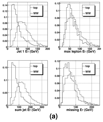
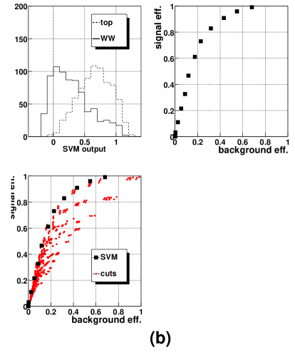
Figure 3: (a) A comparison of the $t\bar{t}$ and WW distributions for the four input variables. (b) Signal efficiency versus background efficiency for SVM compared with conventional cuts.

A training sample with these four variables was used to train the SVM algorithm using the package LIBSVM [15] with a Gaussian kernel function. The target was 0.0 for the WW events and 1.0 for $t\bar{t}$ events. The SVM output on an independent sample of events, shown in Figure 3b, peaks near zero for WW and closer to one for $t\bar{t}$. The figure also shows the performance of the SVM compared to conventional cuts. The SVM performance is about equal to the best performance of the cut-based approach.

Figure 4a compares SVM performance with a Gaussian kernel and a sigmoid kernel. There is no significant difference.

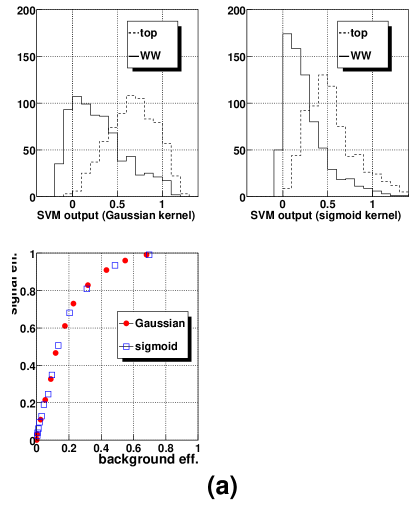
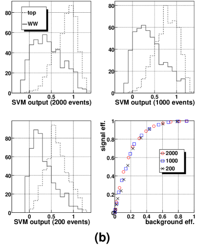
Figure 4: (a) SVM performance of Gaussian kernel versus sigmoid kernel. (b) SVM performance for different numbers of training examples.

Similarly, Figure 4b shows that there is no significant SVM performance difference as the number of the training examples varies from 2000 to 200.

Training time must be considered for any supervised learning algorithm. A very long training time would make it difficult to thoroughly test the algorithm. The table below shows the training time in seconds for different sample sizes. The right column shows the times for the $t\bar{t}$ + WW Monte Carlo samples. The left column shows times for a toy Monte Carlo sample with higher statistics. The training was done with a gaussian kernel on a 1000 MHz Pentium III PC running the Linux operating system. LIBSVM [15] uses a modified Sequential Minimal Optimization (SMO) algorithm that is known to be a fast method to train SVMs. The time scales roughly as the square of the number of training examples. For the top quark study, training time was negligible.

number of events	toy MC time (sec)	$t\bar{t}$ MC time (sec)
200	$<1$	$<1$
400	$<1$	$<1$
1000	$<1$	1
2000	1.5	2
3000	4	6
4000	8
8000	38
16000	149

4 CONCLUSION

SVMs provide nonlinear function approximations by mapping input vectors into a high dimensional feature space where a hyperplane is constructed to separate classes in the data. Computationally intensive calculations in the feature space are avoided through the use of kernel functions. SVMs correspond to a linear method in feature space which makes them theoretically easy to analyze. The grounding in statistical learning theory leads to optimized generalization. Advantages of SVMs include the existence of only one user chosen parameter (aside from kernel parameters) and a unique, global minimum. In an application of SVMs to top quark analysis we found that a straightforward application of the SVM algorithm quickly reproduced the best performance of a cut-based approach. SVMs are a new way to tackle complicated problems in high energy physics and other fields and should be considered as another technique for our multivariate analysis tool box.

References

- [1] Nello Cristianini and John Shawe-Taylor, An Introduction to Support Vector Machines, Cambridge University Press (2000).
- [2] C.J.C. Burges, A Tutorial on Support Vector Machines for Pattern Recognition, Data Mining and Knowledge Discovery, 2(2):1-47 (1998).
- [3] ed. Bernhard Schölkopf, C.J.C. Burges, Alexander J. Smola, Advances in Kernel Methods: Support Vector Machines, MIT Press (1999).
- [4] V. Vapnik and A. Lerner, Pattern recognition using generalized portrait method, Automation and Remote Control, 24 (1963).
- [5] V. Vapnik and A. Chervonenkis, A note on one class of perceptrons, Automation and Remote Control, 25 (1964).
- [6] B.E. Boser, I.M. Guyon, and V.N. Vapnik, A training algorithm for optimal margin classifiers, In D. Haussler, editor, Proceedings of the 5th Annual ACM Workshop on Computational Leraning Theory, pages 144-152, ACM Press (1992).
- [7] C. Cortes and V. Vapnik, Support vector networks, Machine Learning, 20:273-297 (1995).
- [8] V. Vapnik, The Nature of Statistical Learning Theory, Springer Verlag (1995).
- [9] http://www.kernel-machines.org
- [10] F. Abe et al, Phys. Rev. Lett., 74:2626 (1995); A. Abachi et al, Phys. Rev. Lett., 74:2632 (1995).
- [11] E. Berger and H. Contopanagos, Phys. Rev. D, 54:3085 (1996); S. Catani et al, Phys. Lett. B, 378:329 (1996).
- [12] E.Boos et al, CompHEP, Preprint INP MSU 98-41/542, hep-ph/9908288.
- [13] T. Sjöstrand, P. Eden, C. Friberg, L. Lönnblad, G. Miu, S. Mrenna and E. Norrbin, Computer Physics Commun., 135:238 (2001).
- [14] http://www.physics.rutgers.edu/jconway/soft/pgs/pgs.html
- [15] Chih-Chung Chang and Chih-Jen Lin, LIBSVM: a library for support vector machines (2001). Software available at http://www.csie.ntu.edu.tw/cjlin/libsvm