$t\bar{t}$ production cross section in $p\bar{p}$ collisions at $\sqrt{s}=1.8$ TeV

Abstract

Results are presented on a measurement of the $t\bar{t}$ pair production cross section in $p\bar{p}$ collisions at $\sqrt{s}=1.8$ TeV from nine independent decay channels. The data were collected by the DØ experiment during the 1992–1996 run of the Fermilab Tevatron Collider. A total of 80 candidate events is observed with an expected background of $38.8\pm 3.3$ events. For a top quark mass of 172.1 GeV/$c^{2}$, the measured cross section is $5.69\pm 1.21({\rm stat})\pm 1.04({\rm sys})$ pb.

Contents

toc

I Introduction

The observation of the top quark by the CDF and DØ collaborations in the spring of 1995 [3, 4] was the culmination of a long and intensive search that began following the discovery of the $\tau$ lepton in 1976 [5] and the bottom ($b$) quark in 1977 [6]. The discovery of these two particles gave a firm foundation to the existence of a third family, originally proposed by Kobayashi and Maskawa in 1973 to account for the occurrence of $CP$ violation within the standard model [7]. The $b$ quark was shown to possess a charge of $Q_{b}=-{1\over 3}e$ [8, 9, 10] and a weak isospin of $I_{3}=-{1\over 2}$ [11, 12, 13]. Within the standard model (SM), this demanded the existence of a partner to the $b$ quark with a charge of $+{2\over 3}e$ and a weak isospin of $+{1\over 2}$. This partner is called the “top” quark.

Initial searches for the top quark were carried out at $e^{+}e^{-}$ colliders. These searches looked for a narrow resonance (if a bound $t\bar{t}$ state was produced), an increase in the rate of $e^{+}e^{-}\rightarrow{\rm hadrons}$ (if a bound $t\bar{t}$ state was not produced), or events with more spherical angular distributions which differentiate top quark events from the more planar angular distributions expected from the lighter quarks. As shown in Fig. 1(a), experiments at the PETRA [14, 15], TRISTAN [16], and SLC/LEP [17, 18] colliders raised the lower limit on the top quark mass ($m_{t}$) from 15 $\mbox{GeV}/c^{2}$ in 1979 to 45.8 $\mbox{GeV}/c^{2}$ in 1990. In the late 1980’s, in the absence of a signal, the focus of the top quark search shifted from $e^{+}e^{-}$ colliders to $p\bar{p}$ colliders and higher center-of-mass energies. Unlike $e^{+}e^{-}$ colliders, $p\bar{p}$ colliders cannot provide direct limits on the mass of the top quark, but rather upper limits on the $t\bar{t}$ production cross section. By assuming a relationship between mass and cross section (as provided by SM theory), these cross section upper limits can be turned into lower limits on the mass. The UA1 collaboration provided the first such limit in 1988, setting a lower bound on the top quark mass of 45 $\mbox{GeV}/c^{2}$ [19]. This limit was followed in 1990 by an updated limit from UA1 (60 $\mbox{GeV}/c^{2}$) [20] and new limits from UA2 and CDF (69 [21] and 77 [22] $\mbox{GeV}/c^{2}$ respectively). In 1992, CDF raised the lower limit on the top quark mass to 91 $\mbox{GeV}/c^{2}$ [23], and in 1994, DØ set a lower bound of 128 $\mbox{GeV}/c^{2}$ [24].

The first evidence for $t\bar{t}$ production was claimed by the CDF collaboration in April of 1994 [25]. With an integrated luminosity of 19.3 $\>\text{pb}^{-1}$, CDF observed twelve candidate events with an expected background of about six events and estimated a 0.26% probability for the background to fluctuate to at least twelve events. The excess was assumed to be due to $t\bar{t}$ production and the cross section was determined to be $\sigma_{t\bar{t}}=13.9^{+6.1}_{-4.8}$ pb for $m_{t}=174$ $\mbox{GeV}/c^{2}$. The DØ analysis in mid-1994 [26] based on 13.5 $\>\text{pb}^{-1}$ yielded 7 events with an expected background of $3.2\pm 1.1$ events. The DØ and CDF sensitivities (expected number of events for a given cross section) and expected significance (signal to background ratio) were the same. The small excess seen in DØ, if interpreted as being due to $t\bar{t}$ production, gave a cross-section of $6.5\pm 4.9$ pb for $m_{t}=180$ $\mbox{GeV}/c^{2}$. At the time of the top quark discovery the following year, the CDF and DØ collaborations reported $t\bar{t}$ production cross sections of $\sigma_{t\bar{t}}=6.8^{+3.6}_{-2.4}$ pb for $m_{t}=176$ $\mbox{GeV}/c^{2}$ [3] and $\sigma_{t\bar{t}}=6.4\pm 2.2$ pb for $m_{t}=199$ $\mbox{GeV}/c^{2}$ [4], respectively. These results were updated by DØ (1997) and CDF (1998) to $\sigma_{t\bar{t}}=5.5\pm 1.8$ pb [27] for $m_{t}=173.3$ $\mbox{GeV}/c^{2}$ and $\sigma_{t\bar{t}}=7.6^{+1.8}_{-1.5}$ pb [28] for $m_{t}=175$ $\mbox{GeV}/c^{2}$, respectively. In 2001, the CDF collaboration reported $\sigma_{t\bar{t}}=6.5^{+1.7}_{-1.4}$ pb for $m_{t}=175$ $\mbox{GeV}/c^{2}$ [29] as their final $t\bar{t}$ production cross section based on the 1992–1996 run of the Tevatron. The corresponding result from the DØ collaboration, reported in this article, is $\sigma_{t\bar{t}}=5.7\pm 1.6$ pb for $m_{t}=172.1$ $\mbox{GeV}/c^{2}$.

     

FIG. 1.: (a) Lower limit on the top quark mass from 1978 to 1994 [14, 15, 16, 17, 18, 19, 20, 21, 22, 23, 24]. (b) Published $t\bar{t}$ quark cross section results from 1994 to 2001 [25, 3, 4, 27, 28, 29]. The solid triangle marker with the dashed line uncertainty corresponds to the unpublished DØ $t\bar{t}$ cross section in mid-1994 [26].

At the Tevatron center-of-mass energy of 1.8 TeV, top quarks can be produced singly or in pairs. The two cross sections are of similar magnitude [30] but single top quark events are much more difficult to distinguish from background and have not yet been observed [31, 32]. This paper is thus concerned only with $t\bar{t}$ pair production.

FIG. 2.: Lowest order Feynman diagrams for production of $t\overline{t}$ pairs at the Tevatron. At Tevatron energies, the diagram involving quark-antiquark fusion dominates over those involving gluon-gluon fusion.

The $p\bar{p}\rightarrow t\bar{t}$ production cross section can be factorized in terms of the parton-parton cross section and the parton distribution functions for the proton and anti-proton, and is written [33]

$$\sigma(p\bar{p}\rightarrow t\bar{t})=\nobreak\hskip 144.54pt$$ (1)

$$\sum_{i,j}\int dx_{i}dx_{j}f_{i}^{p}(x_{i},\mu^{2})f_{j}^{\bar{p}}(x_{j},\mu^{2}){\hat{\sigma}}_{ij}(\hat{s},\mu^{2},m_{t}),$$ (2)

where the summation indices $i$ and $j$ run over the light quarks and gluons, $x_{i}$ and $x_{j}$ are the momentum fractions of the partons involved in the $p\bar{p}$ collision, $f_{i}^{p}(x_{i},\mu^{2})$ and $f_{j}^{\bar{p}}(x_{j},\mu^{2})$ are the parton distribution functions, and ${\hat{\sigma}}_{ij}(\hat{s},\mu^{2},m_{t})$ is the parton-parton cross section at $\hat{s}=x_{i}x_{j}s$. The renormalization and factorization scales, typically chosen to be the same value $\mu$, are arbitrary parameters with dimensions of energy. The former is introduced by the renormalization procedure and the latter by the splitting of the cross section into perturbative ($\hat{\sigma}$) and nonperturbative ($f^{p},f^{\bar{p}}$) parts. An exact calculation of the cross section would be independent of the choice of $\mu$, but current calculations are performed to finite order in perturbative QCD and are thus dependent on $\mu$, which is usually taken to be of the order of $m_{t}$. Theorists typically estimate the uncertainty introduced by truncating the perturbation expansion by varying $\mu$ over some arbitrary range, usually $m_{t}/2<\mu<2m_{t}$ (the range used for all theoretical cross sections referred to in this paper).

In leading-order QCD (LO), ${\cal O}(\alpha_{s}^{2})$, $t\bar{t}$ production proceeds through $q\bar{q}\rightarrow t\bar{t}$ and $gg\rightarrow t\bar{t}$ processes (see Fig. 2). At $\sqrt{s}=1.8$ TeV, the $q\bar{q}\rightarrow t\bar{t}$ process dominates, contributing 90% of the cross section with the $gg\rightarrow t\bar{t}$ process contributing only 10%. The first calculations of the LO cross section $\hat{\sigma}$ were performed in the late 1970’s [34, 35, 36, 37, 38, 39]. Calculations of the $t\bar{t}$ production cross section at next-to-leading order (NLO), ${\cal O}(\alpha_{s}^{3})$, began to appear in the late 1980’s [40, 41, 42, 43, 44, 45, 46]. The 1990’s saw the introduction of calculations which attempt to estimate the contribution of the higher order terms through a technique known as resummation, in which the sums of the dominant logarithms from soft gluon emission to all orders in perturbation theory are calculated, thus reducing the dependence of the cross section on the value of $\mu$. The first such calculations [47, 48] summed only leading-log (LL) contributions. Increased precision was soon achieved through calculations [49, 50] which incorporated summations through next-to-leading-log (NLL) contributions. The most recent calculations [51, 52] sum contributions through next-to-next-to-leading-log (NNLL). Although the NLL and NNLL calculations have reduced the scale dependence, kinematic-induced ambiguities lead to estimated uncertaintied of about 7% (these latter uncertainties are not included in the theoretical cross section predictions given in this paper).

In the SM, the top quark is expected to decay predominantly into a $W$ boson and a $b$ quark. Decay mechanisms whereby the top quark decays into a charged Higgs boson are not considered here, but are investigated in Refs. [53, 54, 55]. The channels in which the top quark is sought are thus determined by the decay modes of the two $W$ bosons in the $t\bar{t}$ event. The $W$ boson can decay leptonically into an electron, muon, or a $\tau$ lepton (and associated neutrino), and hadronically into $u\overline{d}$, $u\overline{s}$, $u\overline{b}$, $c\overline{d}$, $c\overline{s}$, or $c\overline{b}$ pairs.

FIG. 3.: Expected distributions for $e\mu$ dilepton events of (a) electron $E_{T}$ or muon $p_{T}$, (b) $\hbox to0.0pt{\kern 2.5pt/\hss}E_{T}$, and (c) lepton $\eta\equiv{\rm tanh}^{-1}({\rm cos}\theta)$ (two entries per event). The solid histograms are $t\bar{t}\rightarrow e\mu+X$ signal events (generated with herwig [56] with $m_{t}$ = 175 $\mbox{GeV}/c^{2}$ for $p\bar{p}$ collisions at $\sqrt{s}=1.8$ TeV). The dashed histograms are $Z+{\rm jets}\rightarrow\tau\tau+{\rm jets}\rightarrow e\mu+{\rm jets}$ events (also generated with herwig). All histograms are normalized to unity and all events are required to have $p_{T}^{\ell}>10\mbox{$\mbox{ GeV}/c$},\ \mbox{$\hbox to0.0pt{\kern 2.5pt/\hss}E_{T}$}>10$ GeV, and at least two jets with $E_{T}>15$ GeV and $|\eta|<2.0$.

FIG. 4.: Expected distributions for lepton+jets events of (a) electron $E_{T}$ and muon $p_{T}$ (two entries per event), (b) $\hbox to0.0pt{\kern 2.5pt/\hss}E_{T}$, and (c) lepton $\eta$. The solid histograms are $t\bar{t}$ signal events (generated with herwig with $m_{t}$ = 175 $\mbox{GeV}/c^{2}$ for $p\bar{p}$ collisions at $\sqrt{s}=1.8$ TeV). The dashed histograms are $W+\geq 4$ jet events (generated with vecbos [57]). All histograms are normalized to unity and all events are required to have $p_{T}^{\ell}>15\mbox{$\mbox{ GeV}/c$},\ \mbox{$\hbox to0.0pt{\kern 2.5pt/\hss}E_{T}$}>15$ GeV, and at least four jets with $E_{T}>15$ GeV and $|\eta|<2.0$.

The channels can be classified as follows: the dilepton channel where both $W$ bosons decay leptonically into an electron or a muon ($ee$, $\mu\mu$, $e\mu$), the lepton + jets channel where one of the $W$ bosons decays leptonically and the other hadronically ($e$+jets, $\mu$+jets), and the all-jets channel where both $W$ bosons decay hadronically. This paper will focus primarily on the dilepton and lepton + jets channels. The all-jets channel is discussed in detail in Ref. [58] and is only summarized here. The $t\bar{t}$ channels containing a tau lepton are not explicitly considered, although events containing $\tau\rightarrow e\nu\bar{\nu}$ and $\tau\rightarrow\mu\nu\bar{\nu}$ decays do contribute to the efficiency of all channels containing an electron or a muon. Similarly, the inability to distinguish between a hadronic tau decay and a hadronic jet, contributes to the efficiency of the lepton+jets channels. As is indicated in Figs. 3–6, the leptonic channels are characterized by high transverse-momentum ($p_{T}$) leptons and jets as well as missing transverse momentum ($\hbox to0.0pt{\kern 2.5pt/\hss}E_{T}$) due to high $p_{T}$ neutrinos (see Sec. IV D). The plots show the distributions of several kinematic quantities expected from $t\bar{t}$ decay compared with those expected from the leading background for the $e\mu$ (Figs. 3 and 5) and lepton+jets (Figs. 4 and 6) channels. Initial search strategies are based on previous studies and analyses [59, 25, 60].

FIG. 5.: Expected distributions for $e\mu$ dilepton events of (a and b) the transverse energies of the two leading jets and (c) the jet $\eta$ (two entries per event). The solid histograms are $t\bar{t}\rightarrow e\mu+X$ signal events (generated with herwig with $m_{t}$ = 175 $\mbox{GeV}/c^{2}$ for $p\bar{p}$ collisions at $\sqrt{s}=1.8$ TeV). The dashed histograms are $Z+{\rm jets}\rightarrow\tau\tau+{\rm jets}\rightarrow e\mu+{\rm jets}$ events (also generated with herwig). All histograms are normalized to unity and all events are required to have $p_{T}^{\ell}>10\mbox{$\mbox{ GeV}/c$},\ \mbox{$\hbox to0.0pt{\kern 2.5pt/\hss}E_{T}$}>10$ GeV, and at least two jets with $E_{T}>15$ GeV and $|\eta|<2.0$.

FIG. 6.: Expected distributions for lepton+jets events of (a–d) the transverse energies of the four leading jets and (e) the jet $\eta$ (four entries per event). The solid histograms are $t\bar{t}$ signal events (generated with herwig with $m_{t}$ = 175 $\mbox{GeV}/c^{2}$ for $p\bar{p}$ collisions at $\sqrt{s}=1.8$ TeV). The dashed histograms are $W+\geq 4$ jet events (generated with vecbos). All histograms are normalized to unity and all events are required to have $p_{T}^{\ell}>15\mbox{$\mbox{ GeV}/c$},\ \mbox{$\hbox to0.0pt{\kern 2.5pt/\hss}E_{T}$}>15$ GeV, and at least four jets with $E_{T}>15$ GeV and $|\eta|<2.0$.

The paper is structured as follows: Sec. II gives a brief overview of the DØ detector and indicates those aspects which were employed in the dilepton and lepton+jets analyses. Section III describes the triggers used in the first stage of the event selection. Event reconstruction and particle identification are the subjects of Sec. IV. Section V discusses the simulation of the $t\bar{t}$ signal and background. The dilepton channels are described in Sec. VI and the lepton+jets channels are described in Sec. VII. The all-jets channel is described briefly in Sec. VIII. Section IX discusses the systematic uncertainties. The $t\bar{t}$ cross section results are summarized and tabulated in Sec. X and the conclusions to be drawn from the combined analyses are presented in Sec. XI. Appendix A describes the corrections applied to the jet energy scale; Appendices B and C describe the main-ring veto and recovery; Appendix D presents an independent Neural Network based analysis of the $e\mu$ channel; and Appendix E describes in detail the handling of the uncertainties and the correlations between them.

II The DØ detector

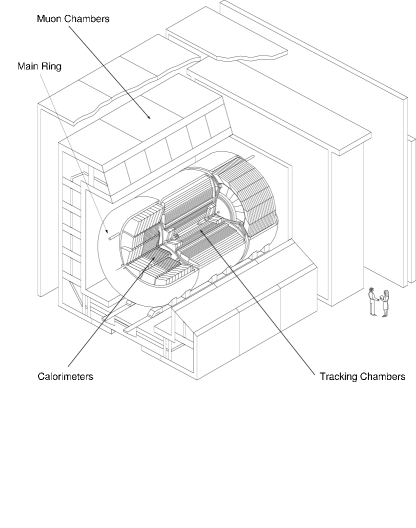
FIG. 7.: Cutaway view of the DØ detector, showing the tracking chambers, calorimetry, and muon system.

DØ is a multipurpose detector designed to study $p\bar{p}$ collisions at high energies. The detector was commissioned at the Fermilab Tevatron Collider during the summer of 1992. The work presented here is based on approximately 125 pb^-1 of data recorded between August 1992 and February 1996. A full description of the detector may be found in Ref. [61]. This section describes briefly those properties of the detector that are relevant for the $t\bar{t}$ production cross section measurements.

Spatial coordinates are specified in a system with the origin at the center of the detector and the positive $z$-axis pointing in the direction of the proton beam. The $x$-axis points radially out of the Tevatron ring and the $y$-axis points upward. Due to the approximate cylindrical symmetry of the detector, it is also convenient to use the variables $r$ (the perpendicular distance from the beamline), $\phi$ (the azimuthal angle with respect to the $x$-axis), and $\theta$ (the polar angle with respect to the $z$-axis). The polar direction is usually described by the pseudorapidity, defined as $\eta\equiv{\rm tanh}^{-1}({\rm cos}\theta$).

In the previous section it was noted that the final state from $t\bar{t}$ decay may contain electrons, muons, jets, and neutrinos. The DØ detector was designed to identify and measure the energy/momentum of all of these objects. As shown in Fig. 7, the detector has three major subsystems: the central tracking chambers, a uranium liquid-argon calorimeter, and a muon spectrometer. The detector design was optimized for high-resolution, nearly hermetic calorimetry that provides the sole measurement of the energies of electrons and jets. Due to the compact design of the calorimeter, the inner tracking volume is relatively small, and there is no central magnetic field.

The central tracking detectors measure the trajectories of charged particles and aid in the identification of electrons. The former function is performed using three wire-chamber systems, and the latter by a transition-radiation detector (TRD). The three wire-chamber systems consist of two concentric cylindrical chambers centered on the interaction point and a set of two forward drift chambers that are situated at the ends of the cylinder. These chambers provide charged-particle tracking over the region $|\eta|<3.2$, measuring the trajectories of charged particles with a resolution of 2.5 mrad in $\phi$ and 28 mrad in $\theta$. The position of the interaction vertex along the beam direction ($z$) can be determined with a resolution of 8 mm. These chambers also measure the track ionization for distinguishing singly charged particles and $e^{+}e^{-}$ pairs from photon conversions. Concentric with, and radially between, the two central chambers is the TRD. By measuring the amount of radiation emitted by single isolated particles as they pass through many thin sheets of polypropylene, this detector aids in the separation of electrons from charged pions and $\pi^{\pm}/\gamma$ overlaps (since the amount of emitted transition radiation is proportional to the value of $E/m$ for the particle). This device provides a factor of ten rejection of pions while retaining 90% of isolated electrons.

Surrounding the central tracking system is the calorimeter, which is composed of plates of uranium and stainless steel/copper absorber surrounded by liquid argon as the sensitive ionization medium. The calorimeter is divided into three parts, the central calorimeter (CC), $|\eta|\leq 1.2$, and two end calorimeters (EC), which together cover the pseudorapidity range $|\eta|<4.2$. Each consists of an inner electromagnetic (EM) section, a fine hadronic (FH) section, and a coarse hadronic (CH) section, housed in a steel cryostat. Each EM section is 21 radiation lengths deep and is divided into four longitudinal segments (layers). The hadronic sections are 7–9 nuclear interaction lengths deep and are divided into four (CC) or five (EC) layers. The outer layer of each hadronic calorimeter is known as the “outer hadronic layer”. The calorimeter is transversely segmented into pseudo-projective towers with $\Delta\eta\times\Delta\phi$ = $0.1\times 0.1$. The third layer of the EM calorimeter, in which the maximum of EM showers is expected, is segmented twice as finely into cells with $\Delta\eta\times\Delta\phi$ = $0.05\times 0.05$. With this fine segmentation, the azimuthal position resolution for electrons with energy above 50 GeV is about 2.5 mm. The energy resolution is $\sigma(E)/E=15\%/\sqrt{E\hbox{(GeV)}}\oplus 0.4\%$ for electrons. For charged pions the resolution is about $50\%/\sqrt{E\hbox{(GeV)}}$ and for jets it is about $80\%/\sqrt{E\hbox{(GeV)}}$ [61]. For minimum bias data, the resolution for each component of $\hbox to0.0pt{\kern 2.5pt/\hss}E_{T}$, $\hbox to0.0pt{\kern 2.5pt/\hss}E_{x}$ and $\hbox to0.0pt{\kern 2.5pt/\hss}E_{y}$, has been measured to be $1.08\hbox{ GeV}+0.019(\Sigma E_{T})$, where $\Sigma E_{T}$ is the scalar sum of the transverse energies in all calorimeter cells. In order to improve the energy resolution for jets that straddle two cryostats, an inter-cryostat detector (ICD) made of scintillator tiles is situated in the space between the EC and CC cryostats. In addition, separate single-cell structures called “massless gaps” (MG) are installed in the intercryostat region in both the CC and EC calorimeters.

The DØ muon detection systems cover $|\eta|\leq 3.3$. Since muons from top quark decays predominantly populate the central region, this work uses only the wide-angle muon spectrometer (WAMUS) which consists of four planes of proportional drift tubes (PDT) in front of magnetized iron toroids with a magnetic field of 1.9 T and two groups of three planes each of proportional drift tubes behind the toroids. The magnetic field lines and the wires in the drift tubes are oriented transversely to the beam direction. The WAMUS covers the region $|\eta|<1.7$ over the entire azimuth, with the exception of the central region below the calorimeter ($|\eta|<1$, $225^{\circ}<\phi<315^{\circ}$), where the inner layer is missing to make room for the calorimeter support-structure. The WAMUS system is divided into the central iron (CF), $|\eta|\leq 1.0$, and end iron (EF), $1.0<|\eta|\leq 1.7$, regions. As will be discussed in Sec. IV B, the EF region was used for only part of the Run 1 data set. The total thickness of the material in the calorimeter and iron toroids varies between 13 and 19 interaction lengths, making background from hadronic punchthrough negligible. The tracking volume is small, thereby reducing backgrounds to prompt muons from in-flight decays of $\pi$ and $K$ mesons. The muon momentum $p$ is measured from its deflection angle in the magnetic field of the toroid. The momentum resolution is limited by multiple Coulomb scattering in the material traversed, the position resolution in the muon chambers, and uncertainty in the magnetic field integral. The typical resolution in $1/p$ is approximately Gaussian and given by

$$\delta(1/p)=0.18(p-2)/p^{2}\oplus 0.003$$ (3)

(with $p$ in GeV/$c$).

As shown in Fig. 7, a separate synchrotron, the Main Ring, sits above the Tevatron and passes through the forward muon system and the outer hadronic section of the calorimeters. During data taking, it was used to accelerate protons for antiproton production. Losses from the Main Ring can deposit energy in the calorimeters and muon system, increasing the instrumental background. As discussed below (Secs. III, VI, and VII), these “Main-Ring events” are removed during the initial selection of all channels. Nevertheless, as discussed in Appendix C, and Secs. VI A and VII A, several analyses have been able to recover some, or all, of these events.

III Triggers

During normal operation, the Tevatron maintains two counter-rotating beams, one consisting of six bunches of protons and the other consisting of six bunches of antiprotons. Proton and antiproton bunches collide at the DØ interaction region every 3.5 $\mu$s (286 kHz). The DØ trigger system is used to select the interesting events and reduce this to a rate of approximately 3–4 Hz, suitable for recording on tape.

The DØ trigger system is composed of three hardware stages (level 0, level 1, and level 1.5) and one software stage (level 2) [61, 60]. The first stage (level 0) consists of hodoscopes of scintillation counters mounted close to the beam on the inner surfaces of the end-calorimeter cryostats and registers hits consistent with a $p\bar{p}$ interaction. This stage is typically used as an input to level 1, but level 0 is not required to fire before an event can proceed to the next stage. In addition, level 0 is used to measure the luminosity. The next stage (level 1) forms fast analog sums of the transverse energies in calorimeter towers. These towers have a size of $\Delta\eta\times\Delta\phi=0.2\times 0.2$ and are segmented longitudinally into electromagnetic and hadronic sections. Based on these sums and patterns of hits in the muon spectrometer, the level 1 trigger decision takes place within the space of a single beam crossing, unless a level 1.5 decision is required (see below). Events accepted at level 1 are digitized and passed on to the level 2 trigger which consists of a farm of 48 general-purpose processors. Software filters running on these processors make the final trigger decision.

At both level 1 and level 2, the triggers are defined in terms of specific objects: electron/photon, muon, jet, $E\kern-5.70007pt\raise 0.81805pt\hbox{/}_{T}$. Tables 1–4 show the triggers used for $t\bar{t}$ event selection. Table 5 shows the triggers used for the muon tag-rate studies discussed in Sec. VII B. As noted above, level 0 is treated as an input term to level 1. Level 1 triggers that do not demand a level 0 pass are denoted “NoL0.”

At level 1, the triggers for electrons (and photons) require the transverse energy in the EM section of the calorimeter to be above programmed thresholds: $E_{T}\equiv E\sin\theta>T$, where $E$ is the energy deposited in the tower, $\theta$ its angle with the beam as viewed from the center of the detector ($z=0$), and $T$ a programmable threshold. The level 2 electron triggers exploit the full segmentation of the EM calorimeter to identify electron showers. Using the trigger towers above threshold at level 1 as seeds, the algorithm forms clusters that include all cells in the four EM layers and the first FH layer in a region of $\Delta\eta\times\Delta\phi=0.3\times 0.3$, centered on the highest $E_{T}$ tower. It checks the shower shape against criteria on the fraction of the energy found in the different EM layers. The $E_{T}$ of the electron is computed based on its energy and the $z$ position of the interaction vertex as determined from the timing of hits in the level 0 hodoscopes. The level 2 algorithm can also apply an isolation requirement or demand an associated track in the central detector.

During the later portion of the run, the level 1.5 trigger processor became available for selecting electrons and photons. For this purpose, the $E_{T}$ of each EM trigger tower passing the level 1 threshold is summed with the neighboring tower that has the most energy and a cut is made on this sum. The hadronic portions of the two towers are also summed and the ratio of the EM transverse energy to the total transverse energy of the two towers is required to be greater than 0.85. The use of a level 1.5 electron trigger is indicated in Tables 1–5 as an “EX” tower in the level 1 column.

TABLE 1.: Electron triggers used in collection of the $t\bar{t}$ signal sample. Column 1 gives the trigger name, column 2 gives the run period for which it was applied, column 3 gives the exposure in $\>\text{pb}^{-1}$ (see text for definition), columns 4 and 5 give the level 1 and level 2 definitions, and column 6 lists the channels that used each trigger. See Appendix C for definitions of the MR veto terms: gb, mrbs, ml, and gc. Channel names are defined in Secs. VI and VII.

Name	Run	Expsr.	Level 1	Level 2	Used by
		($\>\text{pb}^{-1}$)
ele-high	1a	11.0	1 EM tower, $\mbox{$E_{T}$}>10\mbox{$\mbox{ GeV}$}$	1 isolated $e$, $\mbox{$E_{T}$}>20\mbox{$\mbox{ GeV}$}$	$e+\text{jets}$/topo
			GB
ele-jet	1a	14.4	1 EM tower, $\mbox{$E_{T}$}>10\mbox{$\mbox{ GeV}$}$, $|\eta|<2.6$	1 $e$, $\mbox{$E_{T}$}>15\mbox{$\mbox{ GeV}$}$, $|\eta|<2.5$	$ee$, $e\mu$, $e\nu$
			2 jet towers, $\mbox{$E_{T}$}>5\mbox{$\mbox{ GeV}$}$	2 jets ($\Delta R=0.3$), $\mbox{$E_{T}$}>10\mbox{$\mbox{ GeV}$}$, $|\eta|<2.5$	$e+\text{jets}$
			MRBS	$\mbox{${\hbox{$E$\kern-6.00006pt\lower-0.43057pt\hbox{/}}}_{T}^{\text{cal}}$}>10\mbox{$\mbox{ GeV}$}$	$e+\text{jets}/\mu$
ele-jet-high	1b	98.0	1 EM tower, $\mbox{$E_{T}$}>12\mbox{$\mbox{ GeV}$}$, $|\eta|<2.6$	1 $e$, $\mbox{$E_{T}$}>15\mbox{$\mbox{ GeV}$}$, $|\eta|<2.5$	$ee$, $e\mu$, $e\nu$
			2 jet towers, $\mbox{$E_{T}$}>5\mbox{$\mbox{ GeV}$}$, $|\eta|<2.0$	2 jets ($\Delta R=0.3$), $\mbox{$E_{T}$}>10\mbox{$\mbox{ GeV}$}$, $|\eta|<2.5$	$e+\text{jets}$/topo
			ML	$\mbox{${\hbox{$E$\kern-6.00006pt\lower-0.43057pt\hbox{/}}}_{T}^{\text{cal}}$}>14\mbox{$\mbox{ GeV}$}$	$e+\text{jets}/\mu$
ele-jet-high	1c	1.9	1 EM tower, $\mbox{$E_{T}$}>12\mbox{$\mbox{ GeV}$}$, $|\eta|<2.6$	1 $e$, $\mbox{$E_{T}$}>15\mbox{$\mbox{ GeV}$}$, $|\eta|<2.5$	$ee$, $e\mu$, $e\nu$
			2 jet towers, $\mbox{$E_{T}$}>5\mbox{$\mbox{ GeV}$}$, $|\eta|<2.0$	2 jets ($\Delta R=0.3$), $\mbox{$E_{T}$}>10\mbox{$\mbox{ GeV}$}$, $|\eta|<2.5$	$e+\text{jets}/\mu$
			ML	$\mbox{${\hbox{$E$\kern-6.00006pt\lower-0.43057pt\hbox{/}}}_{T}^{\text{cal}}$}>14\mbox{$\mbox{ GeV}$}$
ele-jet-higha	1c	11.0	1 EM tower, $\mbox{$E_{T}$}>12\mbox{$\mbox{ GeV}$}$, $|\eta|<2.6$	1 $e$, $\mbox{$E_{T}$}>17\mbox{$\mbox{ GeV}$}$, $|\eta|<2.5$	$ee$, $e\mu$, $e\nu$
			2 jet towers, $\mbox{$E_{T}$}>5\mbox{$\mbox{ GeV}$}$, $|\eta|<2.0$	2 jets ($\Delta R=0.3$), $\mbox{$E_{T}$}>10\mbox{$\mbox{ GeV}$}$, $|\eta|<2.5$	$e+\text{jets}/\mu$
			1 EX tower, $\mbox{$E_{T}$}>15\mbox{$\mbox{ GeV}$}$	$\mbox{${\hbox{$E$\kern-6.00006pt\lower-0.43057pt\hbox{/}}}_{T}^{\text{cal}}$}>14\mbox{$\mbox{ GeV}$}$
			ML
em1-eistrkcc-ms	1b	93.4	1 EM tower, $\mbox{$E_{T}$}>10\mbox{$\mbox{ GeV}$}$	1 isolated $e$ w/track, $\mbox{$E_{T}$}>20\mbox{$\mbox{ GeV}$}$	$e\nu$
			1 EX tower, $\mbox{$E_{T}$}>15$ GeV	$\mbox{${\hbox{$E$\kern-6.00006pt\lower-0.43057pt\hbox{/}}}_{T}^{\text{cal}}$}>15\mbox{$\mbox{ GeV}$}$	$e+\text{jets}$/topo
			GC, NoL0
mu-ele	1a	13.7	1 EM tower, $\mbox{$E_{T}$}>7\mbox{$\mbox{ GeV}$}$	1 $e$, $\mbox{$E_{T}$}>7\mbox{$\mbox{ GeV}$}$	$e\mu$
			1 $\mu$, $|\eta|<2.4$	1 $\mu$, $\mbox{$p_{T}$}>5\mbox{$\mbox{ GeV}/c$}$, $|\eta|<2.4$
			MRBS
	1b	93.9	1 EM tower, $\mbox{$E_{T}$}>7\mbox{$\mbox{ GeV}$}$	1 $e$, $\mbox{$E_{T}$}>7\mbox{$\mbox{ GeV}$}$, $|\eta|<2.5$	$e\mu$
			1 MX $\mu$, $|\eta|<2.4$	1 $\mu$, $\mbox{$p_{T}$}>8\mbox{$\mbox{ GeV}/c$}$, $|\eta|<2.4$
			GC
mu-ele-high	1c	10.6	1 EM tower, $\mbox{$E_{T}$}>10\mbox{$\mbox{ GeV}$}$, $|\eta|<2.5$	1 $e$, $\mbox{$E_{T}$}>10\mbox{$\mbox{ GeV}$}$, $|\eta|<2.5$	$e\mu$
			1 MX $\mu$, $|\eta|<2.4$	1 $\mu$, $\mbox{$p_{T}$}>8\mbox{$\mbox{ GeV}/c$}$, $|\eta|<1.7$
			GC

TABLE 2.: Muon+jet triggers used in collection of the $t\bar{t}$ signal sample. Column 1 gives the trigger name, column 2 gives the run period for which it was applied, column 3 gives the exposure in $\>\text{pb}^{-1}$ (see text for definition), columns 4 and 5 give the level 1 and level 2 definitions, and column 6 lists the channels that used each trigger. See Appendix C for definitions of the MR veto terms: gb and gc. Channel names are defined in Secs. VI and VII.

Name	Run	Expsr.	Level 1	Level 2	Used by
		($\>\text{pb}^{-1}$)
mu-jet-high	1a	10.2	1 $\mu$, $|\eta|<2.4$	1 $\mu$, $\mbox{$p_{T}$}>8\mbox{$\mbox{ GeV}/c$}$, $|\eta|<1.7$	$e\mu$, $\mu\mu$
			1 jet tower, $\mbox{$E_{T}$}>5\mbox{$\mbox{ GeV}$}$	1 jet ($\Delta R=0.7$), $\mbox{$E_{T}$}>15\mbox{$\mbox{ GeV}$}$	$\mu+\text{jets}$/topo
			GB		$\mu+\text{jets}/\mu$
	1b	66.4	1 $\mu$, $\mbox{$p_{T}$}>7\mbox{$\mbox{ GeV}/c$}$, $|\eta|<1.7$	1 $\mu$, $\mbox{$p_{T}$}>10\mbox{$\mbox{ GeV}/c$}$, $|\eta|<1.7$, scint	$e\mu$, $\mu\mu$
			1 jet tower, $\mbox{$E_{T}$}>5\mbox{$\mbox{ GeV}$}$, $|\eta|<2.0$	1 jet ($\Delta R=0.7$), $\mbox{$E_{T}$}>15\mbox{$\mbox{ GeV}$}$, $|\eta|<2.5$	$\mu+\text{jets}$/topo
			GC		$\mu+\text{jets}/\mu$
mu-jet-cal	1b	88.0	1 $\mu$, $\mbox{$p_{T}$}>7\mbox{$\mbox{ GeV}/c$}$, $|\eta|<1.7$	1 $\mu$, $\mbox{$p_{T}$}>10\mbox{$\mbox{ GeV}/c$}$, $|\eta|<1.7$	$\mu\mu$
			1 jet tower, $\mbox{$E_{T}$}>5\mbox{$\mbox{ GeV}$}$, $|\eta|<2.0$	cal confirm, scint	$\mu+\text{jets}$/topo
			GC	1 jet ($\Delta R=0.7$), $\mbox{$E_{T}$}>15\mbox{$\mbox{ GeV}$}$, $|\eta|<2.5$	$\mu+\text{jets}/\mu$
mu-jet-cent	1b	48.5	1 $\mu$, $|\eta|<1.0$	1 $\mu$, $\mbox{$p_{T}$}>10\mbox{$\mbox{ GeV}/c$}$, $|\eta|<1.0$, scint	$e\mu$, $\mu\mu$
			1 jet tower, $\mbox{$E_{T}$}>5\mbox{$\mbox{ GeV}$}$, $|\eta|<2.0$	1 jet ($\Delta R=0.7$), $\mbox{$E_{T}$}>15\mbox{$\mbox{ GeV}$}$, $|\eta|<2.5$	$\mu+\text{jets}$/topo
			GC		$\mu+\text{jets}/\mu$
	1c	8.9	1 $\mu$, $|\eta|<1.0$	1 $\mu$, $\mbox{$p_{T}$}>12\mbox{$\mbox{ GeV}/c$}$, $|\eta|<1.0$, scint	$e\mu$, $\mu\mu$
			1 jet tower, $\mbox{$E_{T}$}>5\mbox{$\mbox{ GeV}$}$, $|\eta|<2.0$	1 jet ($\Delta R=0.7$), $\mbox{$E_{T}$}>15\mbox{$\mbox{ GeV}$}$, $|\eta|<2.5$
			2 jet towers, $\mbox{$E_{T}$}>3\mbox{$\mbox{ GeV}$}$
			GC
mu-jet-cencal	1b	51.2	1 $\mu$, $|\eta|<1.0$	1 $\mu$, $\mbox{$p_{T}$}>10\mbox{$\mbox{ GeV}/c$}$, $|\eta|<1.0$	$\mu\mu$
			1 jet tower, $\mbox{$E_{T}$}>5\mbox{$\mbox{ GeV}$}$, $|\eta|<2.0$	cal confirm, scint	$\mu+\text{jets}$/topo
			GC	1 jet ($\Delta R=0.7$), $\mbox{$E_{T}$}>15\mbox{$\mbox{ GeV}$}$, $|\eta|<2.5$	$\mu+\text{jets}/\mu$
	1c	11.4	1 $\mu$, $|\eta|<1.0$	1 $\mu$, $\mbox{$p_{T}$}>12\mbox{$\mbox{ GeV}/c$}$, $|\eta|<1.0$	$e\mu$, $\mu\mu$
			1 jet tower, $\mbox{$E_{T}$}>5\mbox{$\mbox{ GeV}$}$, $|\eta|<2.0$	cal confirm, scint
			2 jet towers, $\mbox{$E_{T}$}>3\mbox{$\mbox{ GeV}$}$	1 jet ($\Delta R=0.7$), $\mbox{$E_{T}$}>15\mbox{$\mbox{ GeV}$}$, $|\eta|<2.5$
			GC

TABLE 3.: Jet triggers used in collection the $t\bar{t}$ signal sample. Column 1 gives the trigger name, column 2 gives the run period for which it was applied, column 3 gives the exposure in $\>\text{pb}^{-1}$ (see text for definition), columns 4 and 5 give the level 1 and level 2 definitions, and column 6 lists the channels that used each trigger. See Appendix C for definitions of the MR veto terms: ml, mb, and mrbs. The lepton+jets channels are defined in Sec. VII.

Name	Run	Expsr.	Level 1	Level 2	Used by
		($\>\text{pb}^{-1}$)
jet-3-mu	1b	11.9	3 jet towers, $\mbox{$E_{T}$}>5\mbox{$\mbox{ GeV}$}$	3 jets ($\Delta R=0.7$), $\mbox{$E_{T}$}>15\mbox{$\mbox{ GeV}$}$, $|\eta|<2.5$	$\mu+\text{jets}$/topo
			$\mbox{${\hbox{$E$\kern-6.00006pt\lower-0.43057pt\hbox{/}}}_{T}^{\text{cal}}$}>20\mbox{$\mbox{ GeV}$}$	$\mbox{${\hbox{$E$\kern-6.00006pt\lower-0.43057pt\hbox{/}}}_{T}^{\text{cal}}$}>17\mbox{$\mbox{ GeV}$}$	$\mu+\text{jets}/\mu$
			ML
jet-3-miss-low	1b	57.8	3 large tiles, $\mbox{$E_{T}$}>15$, $|\eta|<2.4$	3 jets ($\Delta R=0.5$), $\mbox{$E_{T}$}>15\mbox{$\mbox{ GeV}$}$, $|\eta|<2.5$	$\mu+\text{jets}$/topo
			3 jet towers, $\mbox{$E_{T}$}>7\mbox{$\mbox{ GeV}$}$, $|\eta|<2.6$	$\mbox{${\hbox{$E$\kern-6.00006pt\lower-0.43057pt\hbox{/}}}_{T}^{\text{cal}}$}>17\mbox{$\mbox{ GeV}$}$	$\mu+\text{jets}/\mu$
			MB
jet-3-l2mu	1b	25.8	3 large tiles, $\mbox{$E_{T}$}>15$, $|\eta|<2.4$	1 $\mu$, $\mbox{$p_{T}$}>6\mbox{$\mbox{ GeV}/c$}$, $|\eta|<1.7$	$\mu+\text{jets}$/topo
			3 jet towers, $\mbox{$E_{T}$}>7\mbox{$\mbox{ GeV}$}$, $|\eta|<2.6$	cal confirm, scint	$\mu+\text{jets}/\mu$
			MB	3 jets ($\Delta R=0.5$), $\mbox{$E_{T}$}>15\mbox{$\mbox{ GeV}$}$, $|\eta|<2.5$
				$\mbox{${\hbox{$E$\kern-6.00006pt\lower-0.43057pt\hbox{/}}}_{T}^{\text{cal}}$}>17\mbox{$\mbox{ GeV}$}$
jet-multi	1a	14.6	4 jet towers, $\mbox{$E_{T}$}>5\mbox{$\mbox{ GeV}$}$	5 jets ($\Delta R=0.3$), $\mbox{$E_{T}$}>10\mbox{$\mbox{ GeV}$}$, $|\eta|<2.0$	all-jets
			MRBS
	1b	96.6	3 large tiles, $\mbox{$E_{T}$}>15\mbox{$\mbox{ GeV}$}$, $|\eta|<2.4$	5 jets ($\Delta R=0.3$), $\mbox{$E_{T}$}>10\mbox{$\mbox{ GeV}$}$, $|\eta|<2.5$	all-jets
			3 jet towers, $\mbox{$E_{T}$}>7\mbox{$\mbox{ GeV}$}$, $|\eta|<2.6$	$\Sigma\mbox{$E_{T}$}>100\mbox{$\mbox{ GeV}$}$ for jets with $|\eta|<2.5$
			and 1 jet tower, $\mbox{$E_{T}$}>3\mbox{$\mbox{ GeV}$}$
			ML
	1c	11.3	3 large tiles, $\mbox{$E_{T}$}>15\mbox{$\mbox{ GeV}$}$, $|\eta|<2.4$	5 jets ($\Delta R=0.3$), $\mbox{$E_{T}$}>10\mbox{$\mbox{ GeV}$}$, $|\eta|<2.5$	all-jets
			3 jet towers, $\mbox{$E_{T}$}>7\mbox{$\mbox{ GeV}$}$, $|\eta|<2.6$	$\Sigma\mbox{$E_{T}$}>120\mbox{$\mbox{ GeV}$}$ for jets with $|\eta|<2.5$
			and 1 jet tower, $\mbox{$E_{T}$}>3\mbox{$\mbox{ GeV}$}$
			ML

TABLE 4.: $E\kern-5.70007pt\raise 0.81805pt\hbox{/}_{T}$ triggers used in collection of the $t\bar{t}$ signal sample. Column 1 gives the trigger name, column 2 gives the run period for which it was applied, column 3 gives the exposure in $\>\text{pb}^{-1}$ (see text for definition), columns 4 and 5 give the level 1 and level 2 definitions, and column 6 notes that these triggers were used only by the $e\nu$ channel. See Appendix C for definitions of the MR veto terms: mrbs and gb. The $e\nu$ channel is defined in Sec. VI.

Name	Run	Expsr.	Level 1	Level 2	Used by
		($\>\text{pb}^{-1}$)
missing-et	1a	13.7	$\mbox{${\hbox{$E$\kern-6.00006pt\lower-0.43057pt\hbox{/}}}_{T}^{\text{cal}}$}>30\mbox{$\mbox{ GeV}$}$	$\mbox{${\hbox{$E$\kern-6.00006pt\lower-0.43057pt\hbox{/}}}_{T}^{\text{cal}}$}>35\mbox{$\mbox{ GeV}$}$	$e\nu$
			1 jet tower, $\mbox{$E_{T}$}>5\mbox{$\mbox{ GeV}$}$, $|\eta|<2.6$
			MRBS
	1b	83.6	$\mbox{${\hbox{$E$\kern-6.00006pt\lower-0.43057pt\hbox{/}}}_{T}^{\text{cal}}$}>40\mbox{$\mbox{ GeV}$}$	$\mbox{${\hbox{$E$\kern-6.00006pt\lower-0.43057pt\hbox{/}}}_{T}^{\text{cal}}$}>40\mbox{$\mbox{ GeV}$}$	$e\nu$
			1 jet tower, $\mbox{$E_{T}$}>5\mbox{$\mbox{ GeV}$}$, $|\eta|<2.6$
			GB
missing-et-high	1c	0.7	$\mbox{${\hbox{$E$\kern-6.00006pt\lower-0.43057pt\hbox{/}}}_{T}^{\text{cal}}$}>50\mbox{$\mbox{ GeV}$}$	$\mbox{${\hbox{$E$\kern-6.00006pt\lower-0.43057pt\hbox{/}}}_{T}^{\text{cal}}$}>50\mbox{$\mbox{ GeV}$}$	$e\nu$
			1 jet tower, $\mbox{$E_{T}$}>5\mbox{$\mbox{ GeV}$}$, $|\eta|<2.6$
			GB

TABLE 5.: Triggers used to study the $\ell$+jets/$\mu$ backgrounds and tag rate function (see Sec. VII B). Column 1 gives the trigger name, column 2 gives the run period for which it was applied, column 3 gives the exposure in $\>\text{pb}^{-1}$ (see text for definition), columns 4 and 5 give the level 1 and level 2 definitions, and column 6 notes that these triggers were used only for $\ell$+jets background studies. See Appendix C for definitions of the MR veto terms: gb, mrbs, ml, and gc. The lepton+jets channels are defined in Sec. VII.

Name	Run	Expsr.	Level 1	Level 2	Used by
		($\>\text{pb}^{-1}$)
jet-min	1b	0.007	1 jet tower, $\mbox{$E_{T}$}>3\mbox{$\mbox{ GeV}$}$	1 jet ($\Delta R=0.3$), $\mbox{$E_{T}$}>20\mbox{$\mbox{ GeV}$}$	$\ell+\text{jets}/\mu$
			GB	prescale = 20	bkg
jet-3-mon	1b	0.92	2 jet towers, $\mbox{$E_{T}$}>5\mbox{$\mbox{ GeV}$}$	3 jets ($\Delta R=0.3$), $\mbox{$E_{T}$}>10\mbox{$\mbox{ GeV}$}$	$\ell+\text{jets}/\mu$
			and 1 jet tower, $\mbox{$E_{T}$}>3\mbox{$\mbox{ GeV}$}$	prescale = 5	bkg
			GB
jet-4-mon	1b	4.6	2 jet towers, $\mbox{$E_{T}$}>5\mbox{$\mbox{ GeV}$}$	4 jets ($\Delta R=0.3$), $\mbox{$E_{T}$}>10\mbox{$\mbox{ GeV}$}$	$\ell+\text{jets}/\mu$
			and 1 jet tower, $\mbox{$E_{T}$}>3\mbox{$\mbox{ GeV}$}$		bkg
			GB
jet-multi	1a	14.6	4 jet towers, $\mbox{$E_{T}$}>5\mbox{$\mbox{ GeV}$}$	5 jets ($\Delta R=0.3$), $\mbox{$E_{T}$}>10\mbox{$\mbox{ GeV}$}$, $|\eta|<2.0$	$\ell+\text{jets}/\mu$
			MRBS		bkg
	1b	96.6	3 large tiles, $\mbox{$E_{T}$}>15\mbox{$\mbox{ GeV}$}$, $|\eta|<2.4$	5 jets ($\Delta R=0.3$), $\mbox{$E_{T}$}>10\mbox{$\mbox{ GeV}$}$, $|\eta|<2.5$	$\ell+\text{jets}/\mu$
			3 jet towers, $\mbox{$E_{T}$}>7\mbox{$\mbox{ GeV}$}$, $|\eta|<2.6$	$\Sigma\mbox{$E_{T}$}>100\mbox{$\mbox{ GeV}$}$ for jets with $|\eta|<2.5$	bkg
			and 1 jet tower, $\mbox{$E_{T}$}>3\mbox{$\mbox{ GeV}$}$
			ML
ele-1-mon	1b	3.1	1 EM tower, $\mbox{$E_{T}$}>7\mbox{$\mbox{ GeV}$}$, $|\eta|<2.5$	1 $e$, $\mbox{$E_{T}$}>16\mbox{$\mbox{ GeV}/c$}$	$\ell+\text{jets}/\mu$
			1 jet tower, $\mbox{$E_{T}$}>3\mbox{$\mbox{ GeV}$}$		bkg
			GC
gis-dijet	1b	93.5	1 EM tower, $\mbox{$E_{T}$}>10\mbox{$\mbox{ GeV}$}$, $|\eta|<2.5$	1 isolated $e/\gamma$, $\mbox{$E_{T}$}>15\mbox{$\mbox{ GeV}/c$}$, $|\eta|<2.0$	$\ell+\text{jets}/\mu$
			1 jet tower, $\mbox{$E_{T}$}>3\mbox{$\mbox{ GeV}$}$	3 jets ($\Delta R=0.7$), $\mbox{$E_{T}$}>15\mbox{$\mbox{ GeV}$}$, $|\eta|<2.0$	bkg
			GC	$\Sigma\mbox{$E_{T}$}>70\mbox{$\mbox{ GeV}$}$ for jets with $|\eta|<2.0$
em1-eistrkcc-esc	1b	91.9	1 EM tower, $\mbox{$E_{T}$}>10\mbox{$\mbox{ GeV}$}$, $|\eta|<2.5$	1 $e$ (no shape cuts), $\mbox{$E_{T}$}>16\mbox{$\mbox{ GeV}$}$	$\ell+\text{jets}/\mu$
			1 jet tower, $\mbox{$E_{T}$}>3\mbox{$\mbox{ GeV}$}$	and 1 isolated $e$ w/track, $\mbox{$E_{T}$}>20\mbox{$\mbox{ GeV}$}$	bkg
			GC

Muon triggers make use of hit patterns in the muon chambers at level 1 and provide the number of muon candidates in different regions of the muon spectrometer. The algorithm searches for hit patterns consistent with a muon originating from the nominal vertex ($z=0$). A level 1.5 processor is also available and can be used to place a $p_{T}$ requirement on the candidates (at the expense of a slightly increased dead time). The use of a level 1.5 muon trigger is indicated in Tables 1–5 as an “MX” muon in the level 1 column.

At level 2, muon tracks are reconstructed using the muon PDT hits and the $z$ position of the interaction vertex from level 0. Valid muon track selection is based on the muon $p_{T}$ and quality requirements (similar to those of Sec. IV B 1). The level 2 muon trigger can also require the presence of a minimum ionizing particle trace in the calorimeter cells along the track. This requirement is indicated in Tables 1–5 by “cal confirm.” In addition, in between Run 1a and Run 1b, layers of scintillator were added to the exterior of the central muon system to veto cosmic rays. The muon triggers indicated by “scint” required the scintillator timing to be in a window of 30 ns before to 70 ns after the beam crossing.

Jet triggers use projective towers of energy deposition in the calorimeter similar to the EM trigger towers but including energy from the hadronic portion of the calorimeter. Level 1 jet triggers require the sum of the transverse energy in the EM and FH sections of a trigger tower (jet tower) to be above programmed thresholds: $E\sin\theta>T$, where $E$ is the energy deposit in the tower, $\theta$ its angle with the beam as seen from the center of the detector ($z=0$), and $T$ a programmable threshold. Alternatively, level 1 can sum the transverse energies within “large tiles” of size $0.8\times 1.6$ in $\eta\times\phi$ and cut on these sums. The level 2 jet algorithm begins with an $E_{T}$-ordered list of towers that are above threshold at level 1. A level 2 jet is formed by placing a cone of radius $\Delta R=\sqrt{\Delta\eta^{2}+\Delta\phi^{2}}$ around the seed tower from level 1. If another seed tower lies within the jet cone, then it is passed over and not allowed to seed a new jet. Using the vertex position measured by the level 0 hodoscopes, the summed $E_{T}$ in all of the towers included in the jet defines the jet $E_{T}$. If any two jet cones overlap, then the towers in the overlap region are added into the jet candidate that was formed first.

${\hbox{$E$\kern-6.00006pt\lower-0.43057pt\hbox{/}}}_{T}^{\text{cal}}$, the missing transverse energy as measured in the calorimeter (see Sec. IV D for definition), can be computed at both level 1 and level 2. At level 1, the $z$ position is assumed to be $z=0$. At level 2, the vertex position from level 0 is used. In the offline reconstruction, the determination of ${\hbox{$E$\kern-6.00006pt\lower-0.43057pt\hbox{/}}}_{T}^{\text{cal}}$ uses the $z$ position as determined by the tracking system. Therefore, the resolution of ${\hbox{$E$\kern-6.00006pt\lower-0.43057pt\hbox{/}}}_{T}^{\text{cal}}$ at the trigger level is significantly poorer than that in the offline reconstruction.

As noted in Sec. II, the Main Ring passes directly through a portion of the outer hadronic calorimeter and muon system. Particles lost from the Main Ring can affect the measurements in these subsystems. Several schemes were employed at the trigger level to reduce or eliminate these effects; these are described in Appendix B.

In addition to the complications introduced by the Main Ring, there are also effects due to multiple interactions. At the mean luminosity (7.5 $\times 10^{30}/{\rm cm}^{2}/{\rm s}$), there are on average 1.3 interactions per bunch crossing. Since the cross section for the production of high-$p_{T}$ interactions is small compared to that for minimum bias, it is very unlikely that more than one high-$p_{T}$ interaction will be present in any given bunch crossing. These additional minimum-bias interactions are usually not included in the Monte Carlo models, but do contribute to mismeasurement of the primary interaction vertex, and therefore to mismeasurement of lepton and jet transverse energies/momenta. The systematic uncertainty due to multiple interactions is discussed in Sec. IX A 7.

The Run 1 data were acquired in three separate run periods: Run 1a from 1992–1993, Run 1b from 1994–1995, and Run 1c from 1995–1996. The period appropriate to each trigger is given in the second column of Tables 1–5.

The integrated luminosity ${\cal L}$ was determined from the counting rate in the level 0 hodoscopes ($R_{L0}$) as

$${\cal L}=\frac{-{\rm ln}(1-\tau R_{L0})}{\tau\sigma_{L0}}$$ (4)

where $\tau=3.5\ \mu s$ is the time interval between beam crossings and $\sigma_{L0}$ is the effective $p\bar{p}$ cross section subtended by the level 0 counters. As described in detail in Ref. [62], $\sigma_{L0}=43.1\pm 1.9{\rm\ mb}$ is obtained from the level 0 trigger efficiency and geometrical acceptance, and from a “world average” $p\bar{p}$ total inelastic cross section of $57.39\pm 1.56$ mb based on results from the CDF [63], E710 [64], and E811 [65] collaborations at Fermilab. The level 0 trigger efficiency is determined using samples of data collected from triggers on random beam crossings and the geometrical acceptance from Monte Carlo studies. It should be noted that the CDF luminosity determinations are based solely on its own measurement of the $p\bar{p}$ inelastic cross section. As a result, luminosities reported by CDF are 6.2% lower than those currently reported by DØ, and consequently, all CDF cross sections are ab initio 6.2% larger than all DØ cross sections. Earlier DØ cross sections (and all previous DØ $t\bar{t}$ cross sections) were based on a $p\bar{p}$ inelastic cross section determined only from the CDF and E710 measurements and are 3.2% lower than current DØ cross sections.

The integrated luminosity (exposure) seen by each of the triggers is given in the third column, labelled “Expsr.,” of Tables 1–5. These values include luminosity losses due to Main-Ring vetos and prescale factors (if appropriate), but do not include the loss to the offline good-beam requirement or losses from runs rejected at later stages of the analysis (see Appendix B for a discussion of the Main-Ring veto schemes).

IV Event reconstruction

A Electron identification

Electrons and positrons are identified by the distinctive pattern of energy that electromagnetic showers deposit in the calorimeter and by the presence of a track from the interaction vertex to the cluster of hit calorimeter cells. The algorithm for clustering calorimeter energy and quantities used to distinguish electrons from backgrounds are described in Ref. [60]. The present analysis includes two additional features: the separation between electrons and backgrounds has been improved by the introduction of a multivariate discriminant, and, for the dilepton channels, use is made of information from the TRD.

The electromagnetic energy scale was calibrated using $Z\rightarrow ee$, $J/\psi\rightarrow ee$, and $\pi^{0}\rightarrow\gamma\gamma$ decays to a precision of 0.08% at $E=M_{Z}/2$ and to 0.6% at $E=20$ GeV [66, 67].

The complete set of identification variables, efficiencies, and misidentification rates is discussed below. Unless otherwise indicated, electrons specified to be in the CC region of the detector span the range $0\leq|\eta|\leq 1.2$ and electrons specified to be in the EC region of the detector span the range $1.2<|\eta|\leq 2.0$ (with the region between the cryostats, $1.2<|\eta|<1.5$, having only a minimal acceptance). Since the central tracking system does not measure the charge of particles, it is not possible to distinguish between electrons and positrons. Therefore, for the remainder of this paper, “electron” shall be used to indicate both electrons and positrons.

1 Electromagnetic energy fraction

Electromagnetic energy clusters are formed by combining calorimeter towers using a nearest-neighbor algorithm with EM tower seeds. The electromagnetic energy fraction $f_{\rm{EM}}$ of a cluster is the ratio of its energy found in EM calorimeter cells to its total energy. All electron candidates are required to have $f_{\rm{EM}}\geq 0.9$.

2 Isolation fraction ($\cal I$)

Electron showers are compact and mostly contained in the core of EM cells within a radius $R=0.2$ in ($\eta$,$\phi$) around the shower center. The isolation fraction $\cal I$ is defined as the ratio of energy in non-core EM and FH cells ($E_{\rm tot}$) within a cone of 0.4 around the center to energy in the EM cluster core ($E_{\rm EM}$)

$${\cal I}={{E_{\rm tot}(0.4)-E_{\rm EM}(0.2)}\over{E_{\rm EM}(0.2)}}.$$ (5)

This quantity tends to be substantially smaller for electrons from the decay of $W$ and $Z$ bosons than for the background, most of which originates from hadronic jets where the electron candidate is usually accompanied by nearby energetic particles.

3 Covariance matrix ($\chi^{2}_{e}$)

A covariance matrix is used to compute a $\chi^{2}$ variable ($\chi^{2}_{e}$) representing the consistency of the cluster shape with that of an electron shower. The covariance matrix uses 41 variables: the fractions of energy deposited in the first, second, and fourth layers of the EM calorimeter; the fractions of energy in each cell of the third EM layer lying in a six by six array around the tower containing the highest energy cell; the logarithm of the cluster energy; and the $z$ position of the interaction vertex. The elements of the covariance matrix depend on $\eta$ and were determined using the døgeant [68] model of the detector (see Sec. V).

4 Cluster-track match significance ($\sigma_{\rm trk}$)

Calorimeter clusters are required to lie along the trajectories of charged particle tracks reconstructed in one of the inner tracking chambers. The cluster-track match significance $\sigma_{\rm trk}$ is a measure of the distance between the cluster centroid and the intersection of the extrapolated track to the third layer of the EM calorimeter.

5 Track ionization ($dE/dx$)

Photons that convert to $e^{+}e^{-}$ pairs before the calorimeter produce pairs of tracks that match an EM cluster well and are too close together to be resolved. Such double tracks can be identified by the amount of ionization produced along the track ($dE/dx$); photon conversions typically deposit twice the charge expected from one minimum ionizing particle.

     

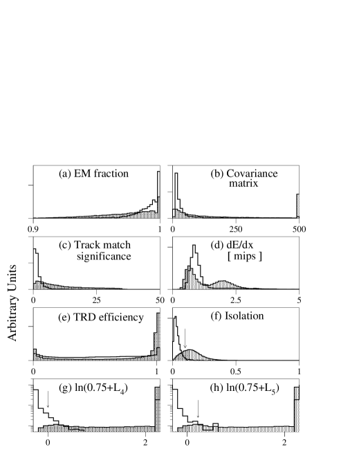
FIG. 8.: (a) – (e) Electron identification variables used in the $L_{4}$ and $L_{5}$ likelihood ratios, (f) Isolation, and (g) and (h) 4-variable and 5-variable likelihood ratios. The open histograms are from electron candidates from $Z\rightarrow e^{+}e^{-}$ events and the shaded histograms are from electron candidates from EM clusters in inclusive jet data (mainly background). Arrows indicate the position of the cuts on isolation, $L_{4}$, and $L_{5}$. All quantities are for the CC region of the detector only.

6 TRD efficiency ($\epsilon_{t}$)

The response of the TRD is characterized by the variable $\epsilon_{t}$:

$$\epsilon_{t}\left(\Delta E\right)={\int_{\Delta E}^{\infty}{\partial N\over\partial E}\left(E\right)dE\over\int_{0}^{\infty}{\partial N\over\partial E}\left(E\right)dE},$$ (6)

where $\Delta E$ is the difference between the total energy recorded in the TRD ($E$) and that recorded in the layer with the largest signal (this is done to reduce sensitivity to $\delta$-rays) and $\partial N\over\partial E$ is the electron energy spectrum from a sample of $W\rightarrow e\nu$ events [69, 70]. Hadrons generally deposit energy mainly in a single layer (giving a small value for $\Delta E$) and electrons deposit energy more evenly (giving a larger value for $\Delta E$). Therefore, hadrons tend to have values of $\epsilon_{t}$ near unity whereas the distribution from electrons is roughly uniform over the allowed range from 0 to 1.

7 Likelihood ratio ($L_{4},L_{5}$)

In order to attain the maximum background rejection while keeping a high efficiency for real electrons, the variables $f_{\rm{EM}}$, $\chi_{e}^{2}$, $\sigma_{\rm trk}$, and $dE/dx$ are combined into an approximate four-variable likelihood ratio $L_{4}$ for the hypotheses that a candidate electron is signal or background. Similarly, the variables $f_{\rm{EM}}$, $\chi_{e}^{2}$, $\sigma_{\rm trk}$, $dE/dx$, and $\epsilon_{t}$ are combined into an approximate five-variable likelihood ratio $L_{5}$. These likelihood ratios are defined using the Neyman-Pearson test for signal ($e$) and background ($b$) hypotheses, where an EM cluster is considered to be an electron if it satisfies

$$L_{n}\equiv\frac{p_{n}(x|b)}{p_{n}(x|e)}<k,$$ (7)

where $x$ is the vector of observables, $p_{n}(x|H)$ is the probability density for $x$ if the hypothesis $H$ is true, and $k$ is the cutoff value. The probability densities are computed by forming the joint likelihood of the four or five variables:

$$p_{4}(x|H) = p(f_{\rm{EM}}|H)\cdot p(\chi_{e}^{2}|H)\cdot p(\sigma_{\rm trk}|H)$$ (9)

$$\cdot p(dE/dx|H),$$

$$p_{5}(x|H) = p(f_{\rm{EM}}|H)\cdot p(\chi_{e}^{2}|H)\cdot p(\sigma_{\rm trk}|H)$$ (11)

$$\cdot p(dE/dx|H)\cdot p(\epsilon_{t}|H),$$

where $p(y|H)$ is the probability density for a single variable $y$ if the hypothesis $H$ is true. These signal and background hypotheses are constructed respectively from inclusive $Z\rightarrow e^{+}e^{-}$ data and inclusive jet production.

The distributions associated with all the above variables for electrons in the CC region of the detector are shown in Fig. 8.

8 Selection

Based on these quantities, four classes of electron candidates are defined:

1. extra-loose electrons are defined as objects satisfying $f_{EM}\geq 0.9$, $\cal{I}$$<0.3$, and $\chi_{e}^{2}<300$.

2. minimal electrons are defined as objects satisfying $f_{EM}\geq 0.9$ and $\cal{I}$$<0.1$.

3. loose electrons are defined as the subset of the extra-loose sample that satisfies the additional requirements $\cal{I}$$<0.1$ and $L_{5}<0.5$ for CC and EC clusters.

4. tight electrons are defined as the subset of the extra-loose sample that satisfies the additional requirements $\cal{I}$$<0.1$ and $L_{4}<0.25(0.3)$ for CC (EC) clusters.

The loose definition is used for the final selection in the dilepton channels ($ee$, $e\mu$, $e\nu$). The tight definition is used for the final selection in the $e$+jets channels.

9 Efficiency

The efficiencies for electron identification are obtained by using the $Z\rightarrow ee$ mass peak. The procedure is based on a sample of events from the em1-eistrkcc-esc trigger (see Table 5) that has two reconstructed electromagnetic clusters, each with $E_{T}\geq 20$ GeV. From this sample, one of the electron candidates, denoted as the “tag,” is required to be a good electron ($\chi^{2}_{e}\leq 100$, ${\cal I}\leq 0.15$). If the other electromagnetic cluster, denoted as the “probe,” satisfies ${\cal I}\leq 0.1$, then the invariant mass of the pair, $m({\rm tag},{\rm probe})$, is recorded. This is done separately for probes in the CC and EC regions of the calorimeter. The number of entries in the $Z$ boson mass window, $80~{}\mbox{$\mbox{GeV}/c^{2}$~{}}<m({\rm tag},{\rm probe})<~{}100~{}\mbox{$\mbox{GeV}/c^{2}$}$, with background subtracted, and in the instrumented region of the central tracking system, defines the number of true electron probes [71]. The track finding efficiency $\varepsilon_{\rm trk}$ is defined as the ratio of the number of true electron probes with a track to the total number of true electron probes. This efficiency varies with the number of interactions per event (see Secs. III and IX A 7). Typical values are $82.7\pm 1.1$ % for electrons in the CC and $85.2\pm 1.0$ % in the EC. The electron identification efficiencies, given in Table 6, are defined by the ratio of the number of true electron probes with a reconstructed track that pass the given identification requirements to the total number of true electron probes with a reconstructed track. These efficiencies do not include geometric factors due to uninstrumented fiducial regions of detector. The geometrical acceptance for electrons in the DØ detector is ($87.6\pm 0.5$)% in the CC and ($79.2\pm 1.4$)% in the EC.

TABLE 6.: Definition of loose and tight electron identification criteria and the corresponding efficiencies (Eff) and misidentification rates ($R_{\rm mis})$.

	Loose		Tight
Region	CC	EC	CC	EC
Def	$L_{5}<.5$	$L_{5}<.5$	$L_{4}<.25$	$L_{4}<.3$
Eff(%)	$88.0\pm 1.6$	$63.8\pm 2.3$	$81.1\pm 1.0$	$51.4\pm 1.8$
$R_{\rm mis}$(%)	$4.6\pm 0.1$	$8.0\pm 0.1$	$2.2\pm 0.1$	$4.0\pm 0.3$

10 Misidentification rate ($R_{\rm mis}$)

The electron misidentification rates ($R_{\rm mis}$) given in Table 6 are measured from a sample of QCD multijet events that contained one electromagnetic cluster passing the extra-loose electron identification requirements defined above. From this sample of extra-loose electron candidates, the fraction passing the loose/tight electron identification is obtained separately for the CC and EC regions of the calorimeter and defined to be the rate for an extra-loose electron candidate to pass the loose/tight criteria. Note that the multijet backgrounds due to electron misidentification are handled differently in the $e$+jets analyses and are discussed in Secs. VII A and VII B.

B Muon identification

Muon tracks are reconstructed using the muon system PDTs. Additional information about the interaction vertex, matching tracks in the central tracker, and minimum ionizing traces left in the calorimeter is also available.

As noted in Sec. II, the decay products from the $t\bar{t}$ pair are emitted at central rapidities and the muon identification is therefore restricted to the central (WAMUS) portion of the DØ muon system, $|\eta|\leq 1.7$. Due to inefficiencies caused by radiation damage, the forward muon region (EF) with $1.0\leq|\eta|\leq 1.7$ was not used in these analyses for Run 1a ($\approx 10\>\text{pb}^{-1}$) or the early part of Run 1b ($\approx 49\>\text{pb}^{-1}$). The chambers were subsequently cleaned and returned to full efficiency for the remainder of Run 1b and Run 1c. In the discussion below, the pre-cleaning period of Run 1b is denoted as “preclean” and the post-cleaning period as “postclean”.

Several categories of muons are used in the analyses. The primary categories correspond to the selection of isolated muons arising dominantly from $W\rightarrow\mu\nu$ decay and non-isolated (tag) muons from $b\rightarrow\mu+X$ decays. Isolation implies a separation of the muon track from nearby jet activity. Isolated muons fall into two categories, tight and loose. The selection requirements for the three types vary slightly over time and are summarized in Tables 7 – 9 for Run 1a, Run 1b(preclean), and Run 1b+c(postclean) respectively. Tight and loose muons share most requirements except that tight muons have the additional requirements of an impact parameter cut and a minimum magnetic field path length (see below). The $p_{T}$ and $\Delta R(\mu,{\rm jet})$ requirements for isolated muons are characteristic of what is expected from $W\rightarrow\mu\nu$ decay. The selection requirements for tag muons are very similar to those for loose-isolated muons except for the lower momentum threshold of $p_{T}\geq 4\mbox{$\mbox{ GeV}/c$~{}}$ and the non-isolation requirement of $\Delta R(\mu,{\rm jet})<0.5$. These $p_{T}$ and $\Delta R$ requirements select muons characteristic of those expected from heavy-flavor decays.

The momentum of the muon is computed from the deflection of the muon trajectory in the magnetized toroid. The momentum calculation uses a least squares method that considers seven parameters: four describing the position and angle of the track before the calorimeter (in both the bend and non-bend views), two describing the effects due to multiple scattering, and the inverse of the muon momentum $1/p$. This seven-parameter fit is applied to sixteen data points: vertex position measurements along the $x$ and $y$ directions, the angles and positions of track segments before and after the calorimeter and outside of the iron, and two angles (one in the bend view, one in the non-bend view) representing the deflection due to multiple Coulomb scattering of the muon in the calorimeter. Energy loss corrections are applied using the restricted energy loss formula parametrized in geant [72].

The muon momentum resolution depends on the amount of material traversed, the magnetic field integral, and the precision of the measurement of the muon bend angle. As noted in Sec. II, the resolution function shown in Eq. 3, was based on studies of $Z\rightarrow\mu\mu$ data. The first term in the resolution function reflects multiple Coulomb scattering in the iron toroids and is the dominant effect for low momentum muons. The second term reflects the resolution of the muon position measurements. The muon momentum scale was calibrated using $J/\psi\rightarrow\mu\mu$ and $Z\rightarrow\mu\mu$ candidates and has an uncertainty of 2.5 %.

The complete set of identification variables and misidentification rates is discussed below.

1 Muon quality ($Q$)

For each found track in the muon system, the reconstruction makes a set of cuts on the number of modules hit, the impact parameters, and the hit residuals. The number of cuts which a track fails is defined as the muon quality, $Q$ (for a perfect track $Q=0$). A similar parameter is also produced by the level 2 trigger. If a track fails more than one (CF) or any (EF) of the cuts on the above quantities, then it is of insufficient quality and is rejected. Tracks that have hits only in the inner layer of the muon system (inside the toroid) are also rejected. This eliminates almost all hadronic punchthrough from the calorimeter into the muon system. If a muon track is not bent by the toroid, muon momentum cannot be measured (as is the case for tracks which only have hits in the inner layers).

2 Calmip/MTC requirement

As a muon passes through the calorimeter it deposits energy through ionization along its path. This minimum ionizing trace should match to the track found in the muon and central tracking systems and can serve as a very powerful tool for the rejection of backgrounds. During the course of the run this was used in two ways. For Run 1a, it is accomplished by checking the energy in the calorimeter towers along the expected path of the muon: For events in which a track match is found in the central tracking system within $\Delta\eta\leq 0.45$ and $\Delta\phi\leq 0.45$ of the muon track, an energy deposit of at least 0.5 GeV is required in the calorimeter towers along the track plus its two nearest neighbor towers; for muons without a central detector track match, at least 1.5 GeV is required (to allow for tracking inefficiencies in the region near $|\eta|\approx$ 1 where the coverage of the central tracking system is incomplete). This requirement is denoted by “calmip” in Tables 7 – 9. For data from Runs 1b and 1c, a more sophisticated procedure is employed. This procedure, denoted “MTC,” is based on muon tracking in the calorimeter. The track from the muon system is used to define a path through the calorimeter to the position of the interaction vertex. A $5\times 5$ road of calorimeter cells is defined along this path. Any cell with an energy two standard deviations above the noise level is counted as hit. The longest contiguous set of hit cells constitutes the calorimeter track. Muon candidates are required to have tracks with hits in at least 70% of the possible layers in the hadronic calorimeter. If a track does not have hits in all the layers, then it is also required that at least one of the nine central cells in the outermost layer of the $5\times 5$ road be hit [71]. These requirements reject both combinatoric background and cosmic rays. The MTC criteria cannot be used on the Run 1a data because the required information is not supplied by the 1a reconstruction. For the $\mu$+jets channels (which uses the tight muon identification criteria) the Run 1a raw data was reprocessed, incorporating the needed information. Thus, in Table 7, MTC refers to the tight identification and the tag identification for the $\mu$ + jets channels and calmip refers to the loose identification and the tag identification for the $e$+jets/$\mu$ channel.

3 Impact parameter (IP)

An impact parameter requirement for the muon trajectory relative to the interaction vertex provides further rejection against cosmic rays and misreconstructed muons. Here $IP_{BV}$ and $IP_{NB}$ are the two-dimensional distances-of-closest approach between the muon and its associated vertex in the bend and non-bend projections respectively. These are combined in quadrature, $IP\equiv\sqrt{IP_{BV}^{2}+IP_{NB}^{2}}$, and $IP$ is required to be less than 20 cm.

4 Minimum magnetic path length ($\int Bdl$)

Muons that pass through the thinner part of the iron toroid near $|\eta|\approx 0.9$ have poorer momentum resolution and may also be contaminated by a small background from punchthrough. Excluding these thin regions, the punchthrough fraction is $<2$ % and is essentially negligible for muons with $p_{T}>5$ $\mbox{ GeV}/c$. The $\int\vec{B}\times\vec{dl}$ requirement ensures that muons traverse enough field ($\geq 1.83$ Tm) to provide an acceptable $p_{T}$ measurement.

TABLE 7.: Definitions of and identification efficiencies for loose, tight, and tag CF ($|\eta|\leq 1.0$) muons for Run 1a. For calmip/MTC: $e\mu$, $\mu\mu$ (loose) and $e$ + jets/$\mu$ (tag) use calmip; $\mu$ + jets/topo (tight) and $\mu$ + jets/$\mu$ (tight and tag) reprocessed the 1a data and therefore use MTC. The two efficiencies given for tag muons reflect inclusion of calmip or MTC requirements respectively.

	$\mu$ id Run 1a (CF)
definition:	Loose	Tight	Tag
$p_{T}^{\mu}\geq$	15	20	4
$Q$ $\leq$	1	1	1
calmip/MTC	yes	yes	yes
$IP\leq$	–	20 cm	–
$\int Bdl\geq$	–	1.83 Tm	–
$\Delta R({\mu,{\rm jet}})$	$\geq 0.5$	$\geq 0.5$	$<0.5$
Eff (%)	$64\pm 6$	$46\pm 7$	$80\pm 6/77\pm 6$

TABLE 8.: Definitions of and identification efficiencies for loose, tight, and tag CF ($|\eta|\leq 1.0$) muons for Run 1b(preclean).

	$\mu$ id Run 1b preclean (CF)
definition:	Loose	Tight	Tag
$p_{T}^{\mu}\geq$	15	20	4
$Q$ $\leq$	1	1	1
MTC	yes	yes	yes
$IP\leq$	–	20 cm	–
$\int Bdl\geq$	–	1.83 Tm	–
$\Delta R({\mu,{\rm jet}})$	$\geq 0.5$	$\geq 0.5$	$<0.5$
Eff (%)	$65\pm 5$	$46\pm 7$	$76\pm 6$

TABLE 9.: Definitions of and identification efficiencies for loose, tight, and tag muons for CF ($|\eta|\leq 1.0$) and EF ($1.0<|\eta|\leq 1.7$) regions for run 1b+c (postclean).

	$\mu$ id Run 1b+c postclean
	Loose		Tight		Tag
definition:	CF	EF	CF	EF	CF	EF
$p_{T}^{\mu}\geq$	15		20		4
$Q$ $\leq$	1	0	1	0	1	0
MTC	yes		yes		yes
$IP\leq$	–	–	20 cm		–	–
$\int Bdl\geq$	–	–	1.83 Tm		–	–
$\Delta R({\mu,{\rm jet}})$	$\geq 0.5$		$\geq 0.5$		$<0.5$
Eff (%)	$73\pm 3$	$68\pm 5$	$49\pm 7$	$52\pm 16$	$84\pm 4$	$62\pm 15$

5 Isolation

A muon is considered isolated if it is well separated from any reconstructed jet. Isolation, or $\Delta R(\mu,{\rm jet})$, is the distance in $(\eta,\phi)$ space between a muon and the nearest 0.5 cone jet with $E_{T}\geq$ 8 GeV.

6 Efficiency

The total muon-finding efficiency is the product of the muon geometrical acceptance and the muon identification efficiency. The muon geometrical acceptance is ($73.7\pm 0.4$)% for the CF and ($64.1\pm 1.1$)% for the EF. The total muon-finding efficiency is well-modeled by a modified version of døgeant. These modifications include input from measured muon resolutions and efficiencies of the PDTs. The muon identification efficiency is obtained from this modified version of døgeant, but is further corrected to account for time dependent detector inefficiencies and incorrect modeling of the muon track finding efficiency. As can be seen in Tables 7 – 9, the muon identification efficiency varies with muon category and run period.

C Jets

Jets are reconstructed using a cone algorithm [60, 73, 74] with cone sizes, $\Delta R(\equiv\sqrt{\Delta\eta^{2}+\Delta\phi^{2}})$, of 0.3 and 0.5. The cone size of $\Delta R=0.3$ is used only in the level-2 trigger and for certain aspects of the all-jets analysis (see Sec. VIII); all other analyses use a cone size of $\Delta R=0.5$ to maximize the efficiency for reconstructing $t\bar{t}$ events. The algorithm is executed as follows. Starting from an $E_{T}$-ordered list of calorimeter towers, the towers within $\Delta R\approx 0.3$ and with $E_{T}>1$ GeV are grouped into preclusters. The energy within a given cone (0.3 and 0.5 for the analyses presented here) centered on the precluster is summed, and a new “$E_{T}$-weighted” center is obtained. Starting with this new center, the process is repeated until the center stabilizes. A jet is required to have $E_{T}>8$ GeV. If two jets share energy, they are combined or split, depending on the fraction of $E_{T}$ shared relative to the $E_{T}$ of the lower $E_{T}$ jet. If the shared fraction exceeds 50%, the jets are combined.

The jet energy resolution is obtained from studies of $E_{T}$ balance in dijet and photon+jet data in different $\eta$ regions [60]. As shown in Fig. 9, the fractional resolution ($\sigma(E_{T})/E_{T}$) in the central region varies from 20% at a jet $E_{T}$ of 30 GeV to 8% at a jet $E_{T}$ of 100 GeV. Resolutions in the other detector regions are similar. The absolute jet energy scale is discussed in the following section.

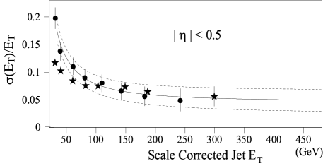
FIG. 9.: Jet $E_{T}$ fractional resolution for $|\eta|<0.5$. The circles and solid line correspond to the nominal resolution; the dotted lines are the systematic uncertainty on the resolution measurement. The stars correspond to resolutions obtained from herwig+døgeant Monte Carlo and are used at high $E_{T}$ where dijet data are not available.

D Missing $E_{T}$ ($\hbox to0.0pt{\kern 2.5pt/\hss}E_{T}$)

Neutrinos escape the detector without interacting. Similarly, muons pass through the calorimeter depositing very little energy. The presence of a high-energy neutrino can be inferred from an imbalance in transverse energy/momentum as measured in the calorimeter and muon systems.

Missing transverse energy in the calorimeter, $\hbox to0.0pt{\kern 2.5pt/\hss}E_{T}^{\rm cal}$, is defined as

$${\hbox{$\hbox to0.0pt{\kern 2.5pt/\hss}E_{T}^{\rm cal}$}}=\sqrt{{\hbox{$\hbox to0.0pt{\kern 2.5pt/\hss}E_{x}^{\rm cal}$}}^{2}+{\hbox{$\hbox to0.0pt{\kern 2.5pt/\hss}E_{y}^{\rm cal}$}}^{2}},$$ (12)

where

$${\hbox{$\hbox to0.0pt{\kern 2.5pt/\hss}E_{x}^{\rm cal}$}}=-\sum_{i}E_{i}{\rm sin}(\theta_{i}){\rm cos}(\phi_{i})-\sum_{j}\Delta E_{x}^{j},$$ (13)

and

$${\hbox{$\hbox to0.0pt{\kern 2.5pt/\hss}E_{y}^{\rm cal}$}}=-\sum_{i}E_{i}{\rm sin}(\theta_{i}){\rm sin}(\phi_{i})-\sum_{j}\Delta E_{y}^{j}.$$ (14)

The first sum is over all cells in the calorimeter and ICD, and the second sum is over the corrections in $E_{T}$ applied to all electrons and jets in the event (see Sec. A). The missing transverse energy ($\hbox to0.0pt{\kern 2.5pt/\hss}E_{T}$) resolution of the calorimeter is parameterized as [60]

$$\sigma(\mbox{${\hbox{$E$\kern-6.00006pt\lower-0.43057pt\hbox{/}}}_{T}^{\text{cal}}$})=1.08{\rm\ GeV}+0.019\sum E_{T},$$ (15)

where $\sum E_{T}$ is the scalar $E_{T}$, which is defined to be the scalar sum of all calorimeter cell $E_{T}$ values.

For events that contain muons, the transverse momentum of the muon is subtracted from ${\hbox{$E$\kern-6.00006pt\lower-0.43057pt\hbox{/}}}_{T}^{\text{cal}}$ to compute the total missing $E_{T}$:

$${\hbox{$\hbox to0.0pt{\kern 2.5pt/\hss}E_{x}$}}={\hbox{$\hbox to0.0pt{\kern 2.5pt/\hss}E_{x}^{\rm cal}$}}-\sum_{i}p^{\mu_{i}}_{x},$$ (16)

$${\hbox{$\hbox to0.0pt{\kern 2.5pt/\hss}E_{y}$}}={\hbox{$\hbox to0.0pt{\kern 2.5pt/\hss}E_{y}^{\rm cal}$}}-\sum_{i}p^{\mu_{i}}_{y}.$$ (17)

V Event simulation

The $t\bar{t}$ signal efficiencies and several rare background rates are computed via Monte Carlo methods. The primary event generator for the signal is herwig [56] with CTEQ3M [75] parton distribution functions (pdf). Tests were also performed with three values of $\Lambda_{\rm QCD}$, and using the MRSA^′ pdfs [76], but no significant variation in $t\bar{t}$ acceptance was seen. herwig chooses the momenta out of the initial hard scattering according to matrix element calculations and models initial and final state gluon emission using leading-log QCD evolution [77]. Each top quark is then made to decay into a $W$ boson and a $b$ quark, and the final state partons are hadronized into jets. Underlying spectator interactions are also included in the model. As a cross-check, acceptances were also computed using the isajet [78] event generator (also using the CTEQ3M pdfs), and the difference between the two is incorporated into the systematic uncertainties on a per channel basis (see Secs. IX A 8 – IX A 9 for details). isajet also chooses the momenta out of the hard scattering based on matrix element calculations, but models the initial and final state gluon emission using Feynman-Field fragmentation [79].

herwig was chosen as the primary generator because it provides good agreement with data in DØ’s color coherence [80] and jet-shape [81] analyses. As discussed in Sec. X, within available statistics, the leptonic top candidates found in the current analysis are in good agreement with expectations from herwig. However, it should be noted that version 5.7 of herwig (the version used for the present analyses) is based on leading-log matrix elements, and is therefore not in complete agreement with higher-order predictions [82, 83].

herwig and isajet samples were generated with top quark masses between 90 and 230 $\mbox{GeV}/c^{2}$. To increase event-processing efficiency, two samples were made for each mass and generator: (1) one in which both of the $W$ bosons were required to decay leptonically ($e,\mu,\tau$), from which only those that resulted in a final state of $ee$, $\mu\mu$, or $e\mu$ were kept, and (2) one in which one of the $W$ bosons was forced to decay leptonically ($e,\mu,\tau$), from which those with no final state electrons or muons were rejected, as were one-half of the dilepton events (in order to preserve the proper branching ratios).

For the dilepton channels, backgrounds from $Z\rightarrow\tau\tau$, $Z\rightarrow\mu\mu$, $WW$, $WZ$, and Drell-Yan production are determined with pythia [84] and with isajet, and the difference used as a measure of systematic uncertainty.

Background levels from $W$+jets production are determined from data. However, as discussed in Sec. VII A, shape information from the vecbos [57] Monte Carlo program is used to determine the survival probability for the latter stages of the $\ell$+jet/topo analyses. For the $\mu$+jets/$\mu$ analysis (see Sec. VII B), vecbos is used to determine the $Z\rightarrow\mu\mu$ background. In both cases, the CTEQ3M [75] pdfs are used. vecbos incorporates the exact tree-level matrix elements for $W$ and $Z$ boson production, with up to four additional partons, and supplies the final state partons. In order to include the effects of additional radiation and underlying events, and to model the hadronization of the final state particles, the vecbos output is passed through herwig’s QCD evolution and fragmentation stages. Since herwig requires information about the color labels of its input partons, both programs were modified to assign color and flavor to the generated partons. The flavors are assigned probabilistically by keeping track of the relative weights of each diagram contributing to the process. The color labels are assigned randomly. To estimate the systematic uncertainty, samples were also generated using isajet, instead of herwig, to fragment the vecbos partons.

The output of an event generator is typically processed through a geant [72] simulation of the detector (døgeant). However, such a detailed simulation is extremely computationally intensive and does not allow for generation of the necessary high-statistics samples. As a compromise, the full døgeant simulation was run on a large sample of electrons and hadrons, and the resultant calorimeter showers were stored in a library [69]. These showers are binned in five quantities representing the input particle:

• $z$ vertex position (6 bins)

• $\eta$ (37 bins matching calorimeter segmentation)

• momentum (7 bins)

• $\phi$ region: The calorimeter is largely symmetric in $\phi$, the exceptions being the cracks between modules in the central electromagnetic calorimeter and the region through which the Main Ring passes in the hadronic calorimeter. Hence, there are only two bins in $\phi$, representing the “good” and “bad” regions.

• particle type: Energy depositions in the calorimeter for electrons/photons and hadrons are stored separately in the shower library.

A total of 1.2 million events was used to populate the library. As events are sent through the library version of the simulation, a shower from the library is selected to model the calorimeter response of each individual particle. The total energy of the shower is scaled by the ratio of the energy of the particle to be simulated to that of the library particle which created the shower. Since the full døgeant simulation for muons is not as time-consuming (owing to their minimum-ionizing nature), muons are not included in the shower library but are instead tracked through the detector just as in non-library version of the simulation.

For the muon system, the efficiency is overestimated and the resolution is underestimated by døgeant. The next step in the simulation procedure therefore smears the muon hit timing information so that the Monte Carlo hit position resolution matches that in $Z\rightarrow\mu\mu$ data, and randomly discards hits to model the chamber inefficiency more accurately. In addition, the muon-system geometry in the Monte Carlo is misaligned in order to reproduce the correct overall momentum resolution.

For several of the analyses, a final step in the simulation models the level 1 and level 2 triggers (trigger simulator). As discussed in Sec. III, the level 1 trigger is a collection of hardware elements interfaced to an AND-OR network. The level 1 simulation therefore consists of simulated trigger elements and a simulated AND-OR network. Level 2 is a software trigger that runs in the online data acquisition environment. The level 2 simulation consists of exactly the same code but has been ported to the offline environment. The level 1 and level 2 simulations are typically used as a single entity, referred to simply as the trigger simulator.

VI Analysis of dilepton events

As discussed in Sec. I, the $ee$, $e\mu$, and $\mu\mu$ dilepton signatures are characterized by two isolated high-$p_{T}$ charged leptons, $\hbox to0.0pt{\kern 2.5pt/\hss}E_{T}$, and two or more jets (from the $b$ quarks and initial and final state radiation). Figures 3 and 5 show Monte Carlo distributions for the lepton and jet $E_{T}/p_{T}$ and $|\eta|$, and the $E\kern-5.70007pt\raise 0.81805pt\hbox{/}_{T}$ expected in $t\bar{t}\rightarrow e\mu$ events with $m_{t}=170~{}\mbox{$\mbox{GeV}/c^{2}$~{}}$. Background events with a similar topology are relatively rare and arise primarily from Drell-Yan production of ($Z/\gamma$)+jets, $WW$+jets, and leptonic $W$+jets events in which the second lepton arises from the misidentification of one of the jets. Therefore, requirements based on the above characteristics form the initial selection for all three channels (see Tables 10, 12, and 14). Additionally, for the $ee$ and $\mu\mu$ channels there are cuts designed to reject $Z\rightarrow ee,\mu\mu$ events.

To attack the remaining background, variables were selected based on a series of cut optimization studies. These are designed to maximize the significance, defined as ${\cal S}\equiv{\rm signal}/\sqrt{{\rm background}}$, and result in the introduction of a new transverse energy variable, defined as

$$H_{T}^{e}\equiv\displaystyle\sum_{\rm jets}E_{T}+({\rm leading\ electron}\ E_{T})$$ (18)

for the $ee$ and $e\mu$ channels and as

$$H_{T}\equiv\displaystyle\sum_{\rm jets}E_{T}$$ (19)

for the $\mu\mu$ channel. The sums are over all jets with $E_{T}\geq 15$ GeV and $|\eta|\leq 2.5$. The optimized $H_{T}^{e}$ and $H_{T}$ cut values are given in the event selection tables in Secs. VI A, VI B, and VI C. An additional result of the optimization studies was the requirement that, for the $ee$, $e\mu$, and $\mu\mu$ channels, there should be at least two jets with $E_{T}\geq 20$ GeV. As discussed below, both of these requirements are very effective in distinguishing $t\bar{t}$ events from background.

In addition to the $ee$, $e\mu$, and $\mu\mu$ channels, a new channel was introduced that is designed to catch dilepton events in which one of the leptons either fails the $p_{T}$ requirement or escapes detection (perhaps by passing through an uninstrumented region of the detector). This “$e\nu$” channel selects events that contain one high-$p_{T}$ electron, significant missing transverse energy, and two or more jets. The analogous $\mu\nu$ channel has not been considered.

Acceptances for all four dilepton channels were computed from Monte Carlo events generated by the herwig program for 24 top quark mass values ($m_{t}$ = 90 – 230 GeV/$c^{2}$) and then passed through the full DØ detector simulation (see Sec. V). The expected number of $t\bar{t}$ events passing the selection for a given channel is

$$N=\sigma_{t\bar{t}}(m_{t})\sum_{i={\rm runs}}\sum_{j={\rm det}}A(i,j,m_{t})\cdot{\mathcal{L}}_{i,j}$$ (20)

where $\sigma_{t\bar{t}}$ is the theoretical $t\bar{t}$ cross section at a top quark mass of $m_{t}$ [47], ${\mathcal{L}}_{i,j}$ is the integrated luminosity for run $i$ and pair of lepton detector regions $j$ (for $ee$ $j$=CC+CC,CC+EC,EC+EC, for $e\mu$ $j$=CC+CF,CC+EF,EC+CF,EC+EF, and for $\mu\mu$ $j$=CF+CF,CF+EF,EF+EF), and the acceptance, $A$, is

$$A=\varepsilon_{\rm trig}\cdot\varepsilon_{\rm pid}\cdot\varepsilon_{\rm sel}\cdot G\cdot{\cal B},$$ (21)

where $\varepsilon_{\rm trig}(i,j,m_{t})$ is the trigger efficiency, $\varepsilon_{\rm pid}(i,j)$ is the efficiency for identifying the two leptons, $\varepsilon_{\rm sel}(i,j,m_{t})$ is the efficiency of the selection criteria, $G(i,j)$ is the geometric acceptance, and ${\cal B}$ is the branching fraction for the sample being studied. Trigger efficiencies are obtained from data or Monte Carlo, depending on the channel, and are discussed in greater detail below. Particle identification efficiencies are obtained from data in the case of electrons (as discussed in Sec. IV A), and from a combination of data and Monte Carlo in the case of muons (as discussed in Sec. IV B). The selection efficiencies $\varepsilon_{\rm sel}$ and geometrical acceptances $G$ are calculated from Monte Carlo. As will be discussed in Sec. X, it is the acceptance, rather than the expected number of $t\bar{t}$ events, that is used to calculate the $t\bar{t}$ cross section. Typical values for acceptance, often denoted as the “efficiency times branching fraction” ($\varepsilon\times{\cal B}$), for all eight leptonic channels, are tabulated in Sec. X for seven values of top quark mass. The numbers of $t\bar{t}$ events expected in the four dilepton channels are tabulated in Secs. VI A,  VI B,  VI C, and  VI D, for the same set of top quark masses. Systematic uncertainties on the acceptances are discussed in Sec. IX.

Whenever possible, backgrounds are measured directly from data. If not, then the backgrounds are determined from Monte Carlo events in which the initial cross sections are normalized either to measured or theoretical values:

$$B=\sigma_{\rm bkg}\sum_{i={\rm runs}}\sum_{j={\rm det}}\Bigl{(}\varepsilon_{\rm trig}\cdot\varepsilon_{\rm pid}\cdot\varepsilon_{\rm sel}\cdot G\Bigr{)}_{i,j}\cdot{\mathcal{L}}_{i,j}$$ (22)

where $\sigma_{\rm bkg}$ is the measured or theoretical cross section for the background under consideration.

A The $ee$ channel

TABLE 10.: Number of observed and expected $ee$ events passing at each cut level of the offline analysis. Expected number of $t\bar{t}$ events are for $m_{t}=172.1\mbox{$\mbox{GeV}/c^{2}$~{}}$. Uncertainties correspond to statistical and systematic contributions added in quadrature.

Number of $ee$ events at each cut level
		Total	mis-id	physics
	Data	sig + bkg	bkg	bkg	$t\bar{t}$
$2e$, $E_{T}^{e}>20$ GeV, + $e$ id + trig				$4168\pm 1243$	$1.9\pm 0.3$
+ 2 jets, $E_{T}^{\rm jet}>15$ GeV	112	$125\pm 36$	$9.0\pm 0.08$	$114\pm 35$	$1.8\pm 0.3$
+ $\mbox{${\hbox{$E$\kern-6.00006pt\lower-0.43057pt\hbox{/}}}_{T}^{\text{cal}}$}>25$ GeV	3	$3.2\pm 1.9$	$0.23\pm 0.06$	$1.5\pm 1.9$	$1.5\pm 0.3$
+ $\mbox{${\hbox{$E$\kern-6.00006pt\lower-0.43057pt\hbox{/}}}_{T}^{\text{cal}}$}>40$ GeV or
$M_{ee}<79$ $\mbox{GeV}/c^{2}$ or $M_{ee}>103$ $\mbox{GeV}/c^{2}$	2	$2.3\pm 0.5$	$0.22\pm 0.06$	$0.62\pm 0.21$	$1.5\pm 0.3$
+ 2 jets, $E_{T}^{\rm jet}>20$ GeV	2	$1.9\pm 0.4$	$0.20\pm 0.05$	$0.39\pm 0.12$	$1.4\pm 0.3$
+ $H_{T}^{e}>120$ GeV	1	$1.7\pm 0.2$	$0.20\pm 0.05$	$0.28\pm 0.09$	$1.2\pm 0.2$

The signature for an event in the $ee$ channel consists of two isolated high-$E_{T}$ electrons, two or more jets (from the $b$ quarks and initial and final state radiation), and significant $E\kern-5.70007pt\raise 0.81805pt\hbox{/}_{T}$ (from the neutrinos). The trigger for this channel was (depending on run period) ele-jet(1a), ele-jet-high(1b), or ele-jet-higha(1c), requiring an electron, 2 jets, and $E\kern-5.70007pt\raise 0.81805pt\hbox{/}_{T}$ at level 2 (see Sec. III for details). As discussed in Appendix C, for this analysis Main-Ring events were corrected and not rejected. Over the complete Run 1 data set, these triggers provided a total integrated luminosity of $130.2\pm 5.6\ {\rm pb}^{-1}$. The event sample passing these triggers consists primarily of misidentified multijet and heavy flavor events.

The backgrounds to this signature arise from Drell-Yan ($Z/\gamma^{*}$) production that results in a dielectron final state ($Z\rightarrow ee$, $Z\rightarrow\tau\tau\rightarrow ee$, and $\gamma^{*}\rightarrow ee$), $WW\rightarrow ee$, and multijet events containing one or more misidentified electrons. The latter background consists primarily of $W(\rightarrow e\nu)$+3 jet events in which one of the jets is misidentified as an electron.

The offline selection cuts and their cumulative effect are summarized in Table 10. After passing the trigger requirement, events are required to have 2 electrons (loose electron identification, see Sec. IV A) with $E_{T}>20$ GeV and $|\eta|\leq 2.5$. This initial selection has an acceptance ($\varepsilon\times{\cal B}$) of ($0.26\pm 0.03$)% (for $m_{t}=170$ GeV/$c^{2}$), and essentially eliminates any background from heavy flavor production and reduces the QCD multijet background to a small fraction of the remaining dominant background from $Z\rightarrow ee$. The number of $Z+n$ jet events is proportional to $\alpha_{s}^{n}$, and a similar steep falloff in jet multiplicity is observed for the other backgrounds present at this stage. Requiring 2 jets with $E_{T}>15$ GeV and $|\eta|\leq 2.5$ significantly reduces backgrounds from $Z$ boson, Drell-Yan and $WW$ production, and QCD multijet events. Most of these ($Z$, Drell-Yan, and QCD multijet) do not contain high-$p_{T}$ neutrinos. Therefore, a hard cut on the $\hbox to0.0pt{\kern 2.5pt/\hss}E_{T}$ brings these events to an even more manageable level. At this point the background is still dominated by $Z\rightarrow ee$ events, so the next step requires that the dielectron invariant mass not be within the mass window of the $Z$ boson (see Table 10). However, since $Z\rightarrow ee$ events have no real $E\kern-5.70007pt\raise 0.81805pt\hbox{/}_{T}$, this cut is only made for events with ${\mbox{$E\kern-5.70007pt\raise 0.81805pt\hbox{/}_{T}$}}<40$ GeV, thereby reclaiming a considerable amount of $t\bar{t}$ efficiency. The final two cuts, $H_{T}^{e}>120$ GeV and $N_{\rm jets}\geq 2$ with $E_{T}^{\rm jet}>20$ GeV and $|\eta^{\rm jet}|\leq 2.5$, are obtained through the optimization procedure discussed in Sec. VI, and provide rejection against the remaining background from $Z\rightarrow\tau\tau$, $WW$, and Drell-Yan production, and QCD multijet events. Table 10 shows the number of data events, expected signal ($m_{t}=172.1$ GeV/$c^{2}$), and expected background surviving at each stage of the selection. It is clear from this table that the $\hbox to0.0pt{\kern 2.5pt/\hss}E_{T}$ requirement greatly reduces the background. This is shown in Fig. 10, where $E\kern-5.70007pt\raise 0.81805pt\hbox{/}_{T}$ is plotted vs $M_{ee}$ for all the major backgrounds (a-d), for $t\bar{t}$ Monte Carlo (e), and for data (f). Because of the presence of two neutrinos, the $WW$ background is not reduced much by the selection on $E\kern-5.70007pt\raise 0.81805pt\hbox{/}_{T}$. It is, however, reduced significantly by the jet and $H_{T}^{e}$ requirements. The effect of the $H_{T}^{e}$ cut on $WW$ events can be seen in Fig. 11(b), which gives the $H_{T}^{e}$ distribution for $t\bar{t}\rightarrow e\mu$ events, but is very similar to that for $t\bar{t}\rightarrow ee$ events. After the above selection, only one $ee$ candidate remains.

FIG. 10.: Scatter plots of $E\kern-5.70007pt\raise 0.81805pt\hbox{/}_{T}$ vs $M_{ee}$ for the $ee$ channel: (a) $Z\rightarrow ee$ events,(b) $Z\rightarrow\tau\tau\rightarrow ee$ MC events, (c) QCD multijet events, (d) $WW\rightarrow ee$ MC events, (e) $t{\bar{t}}\rightarrow ee$ MC signal ($m_{t}=172.1$ GeV/$c^{2}$), and (f) data. The signal region is defined as being above the solid line in each plot.

TABLE 11.: Expected number of $ee$ signal and background events after all cuts in 130.2 ${\rm pb}^{-1}$. Uncertainties are statistical and systematic contributions added in quadrature. The systematic uncertainty on the total background includes correlations among the different background sources.

Expected number of $ee$ events in 130.2 ${\rm pb}^{-1}$
top MC $m_{t}$ ($\mbox{GeV}/c^{2}$)
140	$2.34\pm 0.34$
150	$1.96\pm 0.29$
160	$1.62\pm 0.23$
170	$1.25\pm 0.18$
180	$1.02\pm 0.15$
190	$0.79\pm 0.12$
200	$0.62\pm 0.09$
$Z\rightarrow\tau\tau\rightarrow ee$	$0.08\pm 0.06$
multijet (mis-id $e$)	$0.20\pm 0.05$
$Z\rightarrow ee$	$0.06\pm 0.01$
$WW\rightarrow ee$	$0.09\pm 0.03$
${\rm DY}\rightarrow ee$	$0.06\pm 0.03$
Total background	$0.48\pm 0.10$

The $Z\rightarrow ee$ background is determined entirely from data. As noted above, $Z(\rightarrow ee$)+jets events have no real $\hbox to0.0pt{\kern 2.5pt/\hss}E_{T}$, and due to the excellent electron momentum resolution, any $\hbox to0.0pt{\kern 2.5pt/\hss}E_{T}$ observed in the detector will arise from mismeasurement of jet $E_{T}$ and other noise in the calorimeter. Due to the extremely high rejection power of the $\hbox to0.0pt{\kern 2.5pt/\hss}E_{T}$ requirement on $Z\rightarrow ee$+jet events, a $\hbox to0.0pt{\kern 2.5pt/\hss}E_{T}$ mismeasurement rate is determined from a sample of QCD multijet data selected to closely match the jet requirements in this analysis: $\geq 2$ jets, $E_{T}>20$ GeV, $H_{T}>70$ GeV (where the remaining 50 GeV contribution to the $H_{T}^{e}>120$ GeV is assumed to originate from the highest-$E_{T}$ electron). The fraction of events in this sample that passes the $\mbox{$\hbox to0.0pt{\kern 2.5pt/\hss}E_{T}$}>25$ GeV requirement is taken as the $\hbox to0.0pt{\kern 2.5pt/\hss}E_{T}$ mismeasurement rate (i.e., the fraction of the time that the detector resolution will result in a false $\hbox to0.0pt{\kern 2.5pt/\hss}E_{T}$ signal). Due to a slight dependence on jet multiplicity, the $\hbox to0.0pt{\kern 2.5pt/\hss}E_{T}$ mismeasurement rate is determined as a function of the $\hbox to0.0pt{\kern 2.5pt/\hss}E_{T}$ cut and number of jets $n$ in the event and is found to be ($1.02\pm 0.09$)% for $n=2$, ($0.86\pm 0.02$)% for $n=3$, and ($1.12\pm 0.02$)% for $n=4$ for $\mbox{$\hbox to0.0pt{\kern 2.5pt/\hss}E_{T}$}>25$ GeV; and ($0.20\pm 0.04$)% for $n=2$, ($0.14\pm 0.01$)% for $n=3$, and ($0.17\pm 0.01$)% for $n=4$ for $\mbox{$\hbox to0.0pt{\kern 2.5pt/\hss}E_{T}$}>40$ GeV. These factors are then applied to the number of dielectron events that pass all selection requirements (including the $Z$ boson mass window cut), except for that on $\hbox to0.0pt{\kern 2.5pt/\hss}E_{T}$, to obtain the total expected $Z\rightarrow ee$ background of $0.058\pm 0.013$ events. The systematic uncertainty on this determination is discussed in Sec. IX.

The background from multijet events is also obtained entirely from data. The probability for an extra-loose electron to pass the loose electron identification criteria (see electron misidentification rate discussion in Sec. IV A) is applied to both the full Run 1 sample (not including Main-Ring, MR, events) of dielectron events in which one electron candidate passes the loose identification and the other fails the loose identification but passes the extra-loose identification, and to that where both electron candidates fail the loose identification but pass the extra-loose identification. The resultant misidentification background is then scaled up by the (nonMR + MR)/nonMR luminosity ratio to account for the misidentification background expected in the MR data.

Backgrounds from $Z\rightarrow\tau\tau\rightarrow ee$, $WW\rightarrow ee$, and $\gamma^{*}\rightarrow ee$ are obtained from pythia and isajet Monte Carlo samples via Eq. 22, and are normalized either to experimental or theoretical values.

The $Z\rightarrow\tau\tau\rightarrow ee$ Monte Carlo samples are normalized to DØ’s $Z$ boson cross section measurement and its measurement of $p_{T}^{Z}$ (to obtain more $Z$+jets events and thus enhance the final statistics, generator-level cuts are placed on $p_{T}^{Z}$) [85, 86] and corrected for the $Z\rightarrow\tau\tau$ and $\tau\rightarrow e{\bar{\nu}_{e}}\nu_{\tau}$ branching fractions [87]. The $\gamma^{*}\rightarrow ee$ Monte Carlo sample is likewise normalized to DØ’s measurement of the Drell-Yan ($\gamma^{*}\rightarrow ee$) cross section in the dielectron mass range 30 $\mbox{GeV}/c^{2}$ $\leq M_{ee}\leq$ 60 $\mbox{GeV}/c^{2}$ [88]. The $WW\rightarrow ee$ Monte Carlo samples are normalized to theory [89], and a 10% uncertainty is assigned [90].

For the $Z\rightarrow\tau\tau\rightarrow ee$ background, the associated jet spectrum in pythia, herwig, and isajet does not agree with that found in the $Z\rightarrow ee$ data. This is corrected by incorporating the jet cut survival probabilities from the $Z(\rightarrow ee)$+jet data (where the $H_{T}$ cut is taken as 70 GeV, as in the mismeasured $\hbox to0.0pt{\kern 2.5pt/\hss}E_{T}$ calculation) rather than from Monte Carlo.

As described in the previous section, the $t\bar{t}$ acceptances are computed via Eq. 21 using Monte Carlo events generated with herwig and passed through the DØ detector simulation (see Sec. V). The trigger efficiency is obtained from $Z\rightarrow ee$ data but cross checked with the trigger simulator (see Sec. V). Both approaches result in a trigger efficiency of $99\pm 1$% [70].

The acceptance values after all cuts for seven top quark masses (for all channels) are given in Sec. X. The expected numbers of $t\bar{t}$ events, determined via Eq. 20, are given in Table 11 for each of these seven masses. Finally, a cross section of $2.4\pm 4.6$ pb is obtained for the $ee$ channel.

To test the robustness of the background predictions, comparison is made of data and expectations in regions dominated by background (i.e., at earlier steps along the selection chain). Making use of Eqs. 20 – 22 for the different stages of the selection, Table 10 shows that the expectation from background and $t\bar{t}$ compare well with what is observed in the data at the various stages of the selection procedure.

B The e$\mu$ channel

TABLE 12.: Number of observed and expected $e\mu$ events passing at each cut level of the conventional analysis. Expected number of $t\bar{t}$ events are for $m_{t}=172.1\mbox{$\mbox{GeV}/c^{2}$~{}}$. Uncertainties correspond to statistical and systematic contributions added in quadrature.

Number of $e\mu$ events passing cuts
		Total	Mis-id	Physics
	Data	sig + bkg	bkg	bkg	$t\bar{t}$
$E_{T}^{e}>15$ GeV, $p_{T}^{\mu}>15$ GeV
+ $e$ id + $\mu$ id + trig	130	$93\pm 7$	$50\pm 2$	$39\pm 6$	$4.3\pm 0.9$
+ $\Delta R({\mu,{\rm jet}})>0.5$	60	$59\pm 6$	$17.8\pm 0.9$	$38\pm 6$	$3.4\pm 0.7$
+ $E\kern-5.70007pt\raise 0.81805pt\hbox{/}_{T}$ $>10$ GeV	41	$38\pm 3$	$13.5\pm 0.7$	$21.4\pm 3.3$	$3.4\pm 0.7$
+ $\mbox{${\hbox{$E$\kern-6.00006pt\lower-0.43057pt\hbox{/}}}_{T}^{\text{cal}}$}>20$ GeV	22	$21.8\pm 2.2$	$4.5\pm 0.4$	$14.0\pm 2.1$	$3.2\pm 0.6$
+ $\Delta R({e,\mu})>0.25$	20	$19.5\pm 2.2$	$2.3\pm 0.3$	$14.0\pm 2.0$	$3.2\pm 0.6$
+ 2 jets, $E_{T}^{\rm jet}>15$ GeV	4	$3.4\pm 0.6$	$0.32\pm 0.14$	$0.34\pm 0.09$	$2.7\pm 0.6$
+ $H_{T}^{e}>100$ GeV	4	$2.8\pm 0.5$	$0.11\pm 0.12$	$0.24\pm 0.08$	$2.5\pm 0.5$
+ $H_{T}^{e}>120$ GeV	3	$2.6\pm 0.5$	$0.08\pm 0.12$	$0.20\pm 0.08$	$2.3\pm 0.5$
+ 2 jets, $E_{T}^{\rm jet}>20$ GeV	3	$2.5\pm 0.5$	$0.08\pm 0.12$	$0.19\pm 0.10$	$2.2\pm 0.5$

The signature for an event in the $e\mu$ channel consists of one high-$E_{T}$ isolated electron, one high-$p_{T}$ isolated muon, two or more jets (from the $b$ quarks and initial and final state radiation), and significant $E\kern-5.70007pt\raise 0.81805pt\hbox{/}_{T}$ (from the neutrinos). The trigger for this channel required one of the following level 2 terms to be satisfied:

• ele-jet(1a),ele-jet-high(1b), or ele-jet-higha (1c), which required an electron, 2 jets, and $E\kern-5.70007pt\raise 0.81805pt\hbox{/}_{T}$.

• mu-ele(1a and b) or mu-ele-high(1c), which required an electron and a muon.

• mu-jet-high(1a and b) or mu-jet-cent(1c), which required a muon and a jet.

Details of these triggers are discussed in Sec. III. Main-Ring events are not included in this analysis. Over the complete Run 1 data set, these triggers provided a total integrated luminosity of $112.6\pm 4.8\ {\rm pb}^{-1}$.

The backgrounds to this signature arise from Drell-Yan production of $\tau\tau$ which can lead to $e\mu$ final states ($Z\rightarrow\tau\tau\rightarrow e\mu$ and $\gamma^{*}\rightarrow\tau\tau\rightarrow e\mu$), $WW\rightarrow e\mu$, and multijet events containing an isolated muon and a misidentified electron. The latter background consists primarily of $W(\rightarrow\mu\nu)$+3 jet events, where one of the jets is misidentified as an electron. Backgrounds containing a real electron and a misidentified isolated muon, and those containing both a misidentified electron and a misidentified isolated muon were discussed in Ref. [60] and found to be negligible.

The offline selection cuts and their cumulative effect are summarized in Table 12. After passing the trigger requirement, events are required to have $\geq 1$ electron (loose electron identification, see Sec. IV A) with $E_{T}>15$ GeV, $|\eta|\leq 2.5$ and $\geq 1$ muon (loose muon identification, see Sec. IV B) with $p_{T}>15$ $\mbox{ GeV}/c$. This initial selection has an acceptance ($\varepsilon\times{\cal B}$) of $0.68\pm 0.15$% for $m_{t}=170$ GeV/$c^{2}$. At this stage, the background is dominated by QCD multijet events containing a jet misidentified as an electron and a non-isolated muon from the semi-leptonic decay of a $b$ or $c$ quark. This background is reduced significantly by requiring the muon to be isolated, $\Delta R(\mu,{\rm jet})>0.5$. To further reduce the misidentification background, the next two steps require ${\mbox{$E\kern-5.70007pt\raise 0.81805pt\hbox{/}_{T}$}}>10$ GeV and $\mbox{${\hbox{$E$\kern-6.00006pt\lower-0.43057pt\hbox{/}}}_{T}^{\text{cal}}$}>20$ GeV. The cut on ${\hbox{$E$\kern-6.00006pt\lower-0.43057pt\hbox{/}}}_{T}^{\text{cal}}$ is particularly effective against background from $W(\rightarrow\mu\nu)$+jets events (where one of the jets is misidentified as an electron) due to the fact that ${\hbox{$E$\kern-6.00006pt\lower-0.43057pt\hbox{/}}}_{T}^{\text{cal}}$ provides a measure of the transverse momentum of the $W$ boson since both of its decay products deposit little or no energy in the calorimeter. Studies also show that QCD multijet events that contain a highly electromagnetic jet (misidentified as an electron) which gives rise to an isolated muon from the semi-leptonic decay of a $b$ or $c$ quark, can easily enter this analysis (as can $W(\rightarrow\mu\nu)+$jets events where there is significant bremsstrahlung from the muon as it passes through the EM calorimeter). Such events typically have the $e$ and $\mu$ very close in ($\eta,\phi$) space, and a requirement of $\Delta R({e,\mu})>0.25$ effectively eliminates this class of misidentification background.

After the above requirements, the background is primarily from $Z\rightarrow\tau\tau\rightarrow e\mu$ events and, to a lesser extent, from $WW\rightarrow e\mu$ events. The jets associated with these processes arise from initial state radiation (recoil) and are therefore softer in $E_{T}$ than the $b$ jets in a $t\bar{t}$ event. In addition, as noted above (see Sec. VI A), the number of $Z+n$ jet events is proportional to $\alpha_{s}^{n}$, and a similar steep falloff in jet multiplicity is observed for the Drell-Yan (and presumably $WW$) backgrounds. Requiring two jets with $E_{T}^{\rm jet}>15$ GeV and $|\eta^{\rm jet}|\leq 2.5$ significantly reduces these backgrounds and that from QCD multijet production. The final cuts on $H_{T}^{e}>120$ GeV and $N_{\rm jets}\geq 2$ for $E_{T}^{\rm jet}>20$ GeV and $|\eta^{\rm jet}|\leq 2.0$ are obtained through the optimization procedure discussed in Sec. VI and provide further rejection against the remaining backgrounds. After the above selection, three $e\mu$ candidates remain in the data.

Table 12 shows the number of data events, expected signal ($m_{t}=172.1$ GeV/$c^{2}$), and expected background surviving at each stage of the selection. It is clear from this table that the $H_{T}^{e}$ cut is the most effective cut during the final stages of the analysis. This is also shown in Fig. 11, where the $H_{T}^{e}$ distributions are given for the three major backgrounds (a-c), for $t\bar{t}$ Monte Carlo (d), and for data superimposed on the total background and expected $t\bar{t}$ signal (e).

As in the case of the $ee$ channel, the background from multijet events is obtained entirely from data. The probability for an extra-loose electron to pass the loose electron identification criteria (see misidentification rate discussion in Sec. IV A) is applied to the full Run 1 sample of $e\mu$ events, where the electron candidate passes the extra-loose electron identification but fails the loose electron identification, with all the other kinematic cuts applied. As shown in Table 13, the QCD multijet (misidentified $e$) background is determined to be $0.08\pm 0.12$ events.

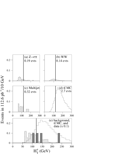
FIG. 11.: $H_{T}^{e}$ distributions for the $e\mu$ channel for expected background (hatched), expected signal (open), and data (solid) after all cuts except $H_{T}^{e}>120$ GeV (shown by solid vertical line) and 2 jets with $E_{T}^{\rm jet}>20$ GeV (corresponding to line 6 of Table 12). Plots (a) – (c) show the individual contributions of the three leading backgrounds and give the expected number of events. Plot (d) gives the expected $t\bar{t}$ contribution ($m_{t}=170$ $\mbox{GeV}/c^{2}$), and plot (e) overlays the total expected background, expected signal, and data ($\times 0.1$).

Background estimates for $Z\rightarrow\tau\tau\rightarrow e\mu$, $WW\rightarrow e\mu$, and $\gamma^{*}\rightarrow e\mu$ events are obtained via Eq. 22 using normalized pythia and isajet Monte Carlo samples. The $Z\rightarrow\tau\tau\rightarrow e\mu$ Monte Carlo samples are normalized to DØ’s measurement of $\sigma(p\bar{p}\to Z+X)B(Z\to ee)$ and the associated measurement of $p_{T}^{Z}$ [85, 86], and incorporate the $Z\rightarrow\tau\tau$, $\tau\rightarrow e{\bar{\nu}_{e}}\nu_{\tau}$, and $\tau\rightarrow\mu{\bar{\nu}_{\mu}}\nu_{\tau}$ branching fractions [87]. The $\gamma^{*}\rightarrow\tau\tau$ Monte Carlo sample is likewise normalized to DØ’s measurement of the Drell-Yan ($\gamma^{*}\rightarrow ee$) cross section in the dielectron mass range 30 $\mbox{GeV}/c^{2}$ $\leq M_{ee}\leq$ 60 $\mbox{GeV}/c^{2}$ [88] also incorporating the $\tau\rightarrow e{\bar{\nu}_{e}}\nu_{\tau}$ and $\tau\rightarrow\mu{\bar{\nu}_{\mu}}\nu_{\tau}$ branching fractions [87]. The $WW\rightarrow e\mu$ Monte Carlo samples are normalized to theory [89], and a 10% uncertainty assigned [90].

As for the $ee$ channel, the $Z\rightarrow\tau\tau\rightarrow e\mu$ Monte Carlo samples are not used to model the jet and $H_{T}^{e}$ requirements. Instead, survival probabilities for these cuts are obtained from $Z(\rightarrow ee)$+jet data.

TABLE 13.: Expected number of $e\mu$ signal and background events in 112.6 ${\rm pb}^{-1}$ after all cuts in the conventional analysis. Uncertainties are statistical and systematic contributions added in quadrature. The systematic uncertainty on the total background includes correlations among the different background sources.

Expected number of $e\mu$ events in 112.6 ${\rm pb}^{-1}$
$t\bar{t}$ MC $m_{t}$ ($\mbox{GeV}/c^{2}$)
140	$4.07\pm 0.88$
150	$3.32\pm 0.72$
160	$2.77\pm 0.60$
170	$2.29\pm 0.49$
180	$1.84\pm 0.40$
190	$1.48\pm 0.32$
200	$1.12\pm 0.24$
$Z\rightarrow\tau\tau\rightarrow e\mu$	$0.10\pm 0.09$
QCD multijet (mis-id $e$)	$0.08\pm 0.12$
$WW\rightarrow e\mu$	$0.08\pm 0.02$
${\rm DY}\rightarrow\tau\tau\rightarrow e\mu$	$0.006\pm 0.004$
Total background	$0.26\pm 0.16$

The $t\bar{t}$ acceptances are computed via Eq. 21 using Monte Carlo events that are generated with herwig and passed through the DØ detector simulation (see Sec. V). The trigger efficiency is obtained from the trigger simulator and is dependent on the detector region of the electron and muon, giving ($95\pm 5)\%$ for CC($e$)CF($\mu$), ($93\pm 5)\%$ for EC($e$)CF($\mu$), ($90\pm 4)\%$ for CC($e$)EF($\mu$), and ($93\pm 5)\%$ for EC($e$)EF($\mu$). The acceptance values after all cuts for seven top quark masses (and for all channels) are given in Sec. X. The expected number of $t\bar{t}$ events passing this selection is determined via Eq. 20 and are given in Table 13 for these same seven masses. Finally, a cross section of $6.8\pm 4.6$ pb is obtained for the $e\mu$ channel.

C The $\mu\mu$ channel

The signature for an event in the $\mu\mu$ channel consists of two isolated high-$p_{T}$ muons, two or more jets (from the $b$ quarks and initial and final state radiation), and significant $E\kern-5.70007pt\raise 0.81805pt\hbox{/}_{T}$ (from the neutrinos). The trigger for this channel required one of the following level 2 terms to be satisfied: mu-jet-high(1a and 1b), mu-jet-cal(1b), mu-jet-cent(1b and 1c), or mu-jet-cencal(1b and 1c). Each of these required a muon and one jet at level 2 (see Sec. III for details). Main-Ring events are not included in this analysis. Over the complete Run 1 data set, these triggers provided a total integrated luminosity of $108.5\pm 4.7\ {\rm pb}^{-1}$.

The backgrounds to this signature arise from Drell-Yan production with dimuon final states ($Z\rightarrow\mu\mu$, $Z\rightarrow\tau\tau\rightarrow\mu\mu$, and $\gamma^{*}\rightarrow\mu\mu$), $WW\rightarrow\mu\mu$, and multijet events containing misidentified isolated muons. The latter background consists primarily of four-jet events where the semi-leptonic decay of $b$ and/or $c$ quarks result in two muons that pass the isolation requirement, and of $W(\rightarrow\mu\nu)$+3 jet events where one of the jets gives rise (through the semi-leptonic decay of a $b$ or $c$ quark) to a muon that passes the isolation requirement.

TABLE 14.: Number of observed and expected $\mu\mu$ events passing at each cut level of the offline analysis. Shown are results for Run 1b+1c (CF-CF) only. Expected number of $t\bar{t}$ events are for $m_{t}=172.1\mbox{$\mbox{GeV}/c^{2}$~{}}$. Uncertainties correspond to statistical and systematic contributions added in quadrature.

number of $\mu\mu$ events passing cuts
		Total	Mis-id	Physics
	Data	sig + bkg	bkg	bkg	$t\bar{t}$
$2\mu$, $p_{T}^{\mu}>15$ GeV/$c$, + $\mu$ id
+ trig + 1 jet, $E_{T}^{\rm jet}>20$ GeV	606	–	–	$174\pm 50$	$1.6\pm 0.2$
+ $\Delta\phi(\vec{\mu}_{1},\vec{\mu}_{2})<165^{\circ}$ for $|\eta_{\mu_{1}}+\eta_{\mu_{2}}|<0.3$	207	–	–	$146\pm 42$	$1.5\pm 0.2$
+ $M_{\mu\mu}>10$ $\mbox{GeV}/c^{2}$ (J$/\psi$ rej)	165	$187\pm 43$	$40\pm 9$	$146\pm 42$	$1.5\pm 0.2$
+ $\Delta R({\mu,{\rm jet}})>0.5$	105	$136\pm 39$	$0.70\pm 0.33$	$134\pm 39$	$0.9\pm 0.1$
+ 2nd jet, $E_{T}^{\rm jet}>20$ GeV	19	$13.6\pm 8.0$	$0.22\pm 0.10$	$12.7\pm 8.0$	$0.72\pm 0.09$
+ $H_{T}>100$ GeV	6	$5.1\pm 3.3$	$0.03\pm 0.02$	$4.5\pm 3.3$	$0.53\pm 0.07$
+$Z$ fit prob$(\chi^{2})<1$ %	1	$0.9\pm 0.3$	$0.03\pm 0.02$	$0.42\pm 0.16$	$0.48\pm 0.06$

The offline selection cuts and their cumulative effect are summarized in Table 14. After passing the trigger requirement, events are required to have two muons (loose muon identification, see Sec. IV B) with $p_{T}>15$ $\mbox{ GeV}/c$ and $|\eta|\leq 1.0$ ($|\eta|\leq 1.7$ in Run 1bc postclean) and one jet with $E_{T}^{\rm jet}>20$ GeV and $|\eta|\leq 2.5$. This initial selection has an acceptance ($\varepsilon\times{\cal B}$) of 0.35% ($m_{t}=170$ GeV/$c^{2}$). At this stage, the dominant background is from cosmic rays. This is minimized by rejecting tracks that are back-to-back in both $\eta$ and $\phi$:

$$\Delta\phi(\vec{\mu}_{1},\vec{\mu}_{2})<165^{\circ}{\rm\ for\ }|\eta(\vec{\mu}_{1})+\eta(\vec{\mu}_{2})|<0.3.$$ (23)

It is necessary to exclude background from J/$\psi\rightarrow\mu\mu$. As discussed below, the muon momentum resolution prohibits an efficient cut on $M_{\mu\mu}$ at the $Z$ boson mass peak. However, at lower muon $p_{T}$, it is an effective quantity and is used to reject low-mass pairs resulting from high-$p_{T}$ J/$\psi$ production with recoil jets: $M_{\mu\mu}>10\ \mbox{$\mbox{GeV}/c^{2}$~{}}$ is required. At this stage, the background is dominated by QCD multijet events rich in heavy flavor with muons originating from semi-leptonic decays of $b$ or $c$ quarks. By requiring both muons to be isolated ($\Delta R(\mu,{\rm jet})>0.5$), this background is reduced to a negligible level. The remaining background is mainly from events containing isolated dimuons from $Z/\gamma^{*}$ and $WW$ production. The jets associated with these processes arise from recoil and are thus softer in $E_{T}$ than the $b$ jets in a $t\bar{t}$ event. Also, as noted in Sec. VI A, the number of $Z+\geq n$ jet events is proportional to $\alpha_{s}^{n}$, and a similar steep falloff in jet multiplicity is observed for the Drell-Yan and $WW$ backgrounds. The next step in the analysis therefore requires a second jet with $E_{T}>20$ GeV and $|\eta|\leq 2.5$, reducing the dimuon background from these sources. The requirement of $H_{T}>100$ GeV is obtained through the optimization procedure, as discussed in Sec. VI, and provides further rejection against the remaining background, leaving only the contribution from $Z\rightarrow\mu\mu$ at a non-negligible level.

As noted above, because of limitations on the momentum resolution of the DØ muon system, the invariant mass peak of the $Z$ boson is smeared and a simple cut on $M_{\mu\mu}$ is ineffective in reducing this background. Instead, rejection is achieved using the result of a $\chi^{2}$ minimization procedure that involves a refitting of the muon momenta with a constraint that the transverse momentum of the dimuon system balance the remaining transverse energy in the event:

$$\chi^{2}= \frac{\bigl{(}\frac{1}{p_{\mu 1}}-\frac{1}{p^{0}_{\mu 1}}\bigr{)}^{2}}{\sigma^{2}\bigl{(}\frac{1}{p_{\mu 1}}\bigr{)}}+\frac{\bigl{(}\frac{1}{p_{\mu 2}}-\frac{1}{p^{0}_{\mu 2}}\bigr{)}^{2}}{\sigma^{2}\bigl{(}\frac{1}{p_{\mu 2}}\bigr{)}}$$ (24)

$$+\frac{\bigl{(}\mbox{$\hbox to0.0pt{\kern 2.5pt/\hss}E_{x}^{\rm cal}$}-\bigl{(}p^{0}_{\mu 1}\bigr{)}_{x}-\bigl{(}p^{0}_{\mu 2}\bigr{)}_{x}\bigr{)}^{2}}{\sigma^{2}\bigl{(}\mbox{$\hbox to0.0pt{\kern 2.5pt/\hss}E_{x}^{\rm cal}$}\bigr{)}}$$ (25)

$$+\frac{\bigl{(}\mbox{$\hbox to0.0pt{\kern 2.5pt/\hss}E_{y}^{\rm cal}$}-\bigl{(}p^{0}_{\mu 1}\bigr{)}_{y}-\bigl{(}p^{0}_{\mu 2}\bigr{)}_{y}\bigr{)}^{2}}{\sigma^{2}\bigl{(}\mbox{$\hbox to0.0pt{\kern 2.5pt/\hss}E_{y}^{\rm cal}$}\bigr{)}},$$ (26)

with the constraint that $M_{\mu\mu}=M_{Z}$:

$$M_{Z}^{2}=2(p^{0}_{\mu 1}p^{0}_{\mu 2}-{\vec{p}}^{0}_{\mu 1}\cdot{\vec{p}}^{0}_{\mu 2})$$ (27)

where $p_{\mu i}$ is the measured momentum for the $i$-th muon, $p_{\mu i}^{0}$ is the fitted value of $p_{\mu i}$, $\sigma(\frac{1}{p_{\mu i}})$ is the measured muon momentum resolution (see Eq. 3), $\hbox to0.0pt{\kern 2.5pt/\hss}E_{x}^{\rm cal}$ and $\hbox to0.0pt{\kern 2.5pt/\hss}E_{y}^{\rm cal}$ are the $x$ and $y$ components of $\hbox to0.0pt{\kern 2.5pt/\hss}E_{T}^{\rm cal}$, and $\sigma(\mbox{$\hbox to0.0pt{\kern 2.5pt/\hss}E_{x}^{\rm cal}$})$ and $\sigma(\mbox{$\hbox to0.0pt{\kern 2.5pt/\hss}E_{y}^{\rm cal}$})$ are their measured resolutions (see Eq. 15). This $\chi^{2}$ is minimized as a function of $p^{0}_{\mu 1}$ and $p^{0}_{\mu 2}$. An event is considered to be a $Z\rightarrow\mu\mu$ candidate, and is thus rejected, if ${\rm Prob}(\chi^{2})>0.01$. This procedure is also used to remove $Z\rightarrow\mu\mu$ background from the $t\bar{t}\rightarrow\mu+{\rm jets}+\mu$ tag channel (see Sec. VII B).

Table 14 shows the number of observed events, expected signal (for $m_{t}=172.1$ GeV/$c^{2}$), and expected background surviving at each stage of the selection. It is clear from this table that the $H_{T}$ and ${\rm Prob}(\chi^{2})$ cuts provide significant background rejection in the final stages of the analysis. This is shown in Fig. 12, where $H_{T}$ vs ${\rm Prob}(\chi^{2})$ is plotted for $Z\rightarrow\mu\mu$ and $Z\rightarrow\tau\tau\rightarrow\mu\mu$ MC events (a,b), for $t\bar{t}$ MC events (c), and for data (d).

FIG. 12.: Scatter plots of $H_{T}$ vs Prob($\chi^{2}$) for the $\mu\mu$ channel: (a) $Z\rightarrow\mu\mu$ background, (b) $Z\rightarrow\tau\tau\rightarrow\mu\mu$ background, (c) $t{\bar{t}}\rightarrow\mu\mu$ signal, and (d) data. The signal region is shown in the upper left corner of each plot (Prob($\chi^{2}$) $<$ 1%, $H_{T}>100$ GeV).

One ${t\bar{t}}\rightarrow\mu\mu$ candidate survives the above selection. Both muons in the event are central, and each track has the maximum of ten hits in the muon chambers, the case where the momentum resolution is best modeled and understood. An interesting feature of this event is that all the muons and jets are in one hemisphere in $\phi$ in the detector, leaving only $E\kern-5.70007pt\raise 0.81805pt\hbox{/}_{T}$ in the other half; this topology is highly unlikely to come from the main background of $Z\rightarrow\mu\mu$ production.

The background from multijet events is determined entirely from data. The probability for a jet to give rise to an isolated muon is determined separately for the CF and EF regions of the muon system using a sample of of multijet events. These probabilities are then applied to the jets in a sample of muon (loose identification, see Sec. IV B) + jet events to obtain the background expected from $W(\rightarrow\mu\nu)$+jets, QCD multijet production, and $Z\rightarrow\tau\tau\rightarrow\mu$ + hadrons where the second muon originates from the semi-leptonic decay of a $b$ or $c$ quark from initial or final state radiation.

In a manner analogous to the background calculations used for the $ee$ and $e\mu$ channels, backgrounds from $Z\rightarrow\mu\mu$, $Z\rightarrow\tau\tau\rightarrow\mu\mu$, $WW\rightarrow\mu\mu$, and $\gamma^{*}\rightarrow\mu\mu$ are obtained via Eq. 22 from pythia and isajet Monte Carlo samples which are normalized to experimental or theoretical values. In particular, the $Z\rightarrow\tau\tau\rightarrow\mu\mu$ MC samples are normalized to the DØ $Z$ boson cross section measurement but incorporate $Z\rightarrow\tau\tau$ and $\tau\rightarrow\mu{\bar{\nu}_{\mu}}\nu_{\tau}$ branching fractions from elsewhere [87]. Similarly, the $\gamma^{*}\rightarrow\mu\mu$ Monte Carlo sample is normalized to DØ’s measurement of the Drell-Yan ($\gamma^{*}\rightarrow ee$) cross section in the dielectron mass range 30 $\mbox{GeV}/c^{2}$ $\leq M_{ee}\leq$ 60 $\mbox{GeV}/c^{2}$ [88]. The $WW\rightarrow\mu\mu$ Monte Carlo sample is normalized to theory [89] and a 10% uncertainty assigned [90].

As for the $ee$ and $e\mu$ channels, the $Z\rightarrow\tau\tau\rightarrow\mu\mu$ Monte Carlo samples are not used to model the jet and $H_{T}$ requirments. Instead, survival probabilities for these cuts are obtained from $Z(\rightarrow ee)$+jet data.

As described in Sec. VI, the $t\bar{t}$ acceptances are computed via Eq. 21 using Monte Carlo events that are generated with herwig and passed through the DØ detector simulation (Sec. V). The trigger efficiency is computed using data-derived trigger turn-on curves applied to $t\bar{t}$ Monte Carlo and is determined to be ($95\pm 5$)%. The acceptance values after all cuts for seven top quark masses (and for all channels) are given in Sec. X. The expected numbers of $t\bar{t}$ events passing this selection are determined via Eq. 20 and are given in Table 15 for these same seven masses. Finally, a cross section of $2.1\pm 8.8$ pb is obtained for the $\mu\mu$ channel.

To test the robustness of the background predictions, comparisons are made between the data and expectations in regions dominated by background (i.e., at earlier steps along the selection chain). Equations. 20 – 22 give, for the different stages of the selection, the results in Table 14, which show that that the expectation from background and $t\bar{t}$ compare well with what is observed in the data at the various stages of the selection procedure.

TABLE 15.: Expected number of $\mu\mu$ signal and background events after all cuts in 108.5 ${\rm pb}^{-1}$. Uncertainties are statistical and systematic contributions added in quadrature. The systematic uncertainty on the total background includes correlations among the different background sources.

Expected number of $\mu\mu$ events in 108.5 ${\rm pb}^{-1}$
$t\bar{t}$ MC $m_{t}$ ($\mbox{GeV}/c^{2}$)
140	$1.02\pm 0.15$
150	$0.88\pm 0.13$
160	$0.78\pm 0.11$
170	$0.67\pm 0.09$
180	$0.54\pm 0.08$
190	$0.44\pm 0.06$
200	$0.33\pm 0.05$
$Z\rightarrow\tau\tau\rightarrow\mu\mu$	$0.03\pm 0.03$
QCD multijet (mis-id $\mu$)	$0.07\pm 0.01$
$Z\rightarrow\mu\mu$	$0.58\pm 0.22$
$WW\rightarrow\mu\mu$	$0.007\pm 0.004$
${\rm DY}\rightarrow\mu\mu$	$0.07\pm 0.04$
Total background	$0.75\pm 0.24$

D The $e\nu$ channel

The $e\nu$ channel is based on the assumption that one of the $W$ bosons decays to $e\nu$ and that the remaining $t\bar{t}$ decay products conspire to give rise to significant ${\hbox{$E$\kern-6.00006pt\lower-0.43057pt\hbox{/}}}_{T}^{\text{cal}}$ ($>50$ GeV). As can be inferred from Figs. 3 and 4, this is most probable for $ee$ and $e\mu$ events but will also occur in some fraction of the $e$+jets events. To eliminate overlap with the dilepton channels, it is further assumed that for $e\mu$($ee$) events, the muon (second electron) is either too low in $p_{T}$($E_{T}$) to pass the selection or escapes detection. The signature for an event in the $e\nu$ channel is therefore one, and only one, high-$E_{T}$ electron, two or more jets (from the $b$ quarks and initial and final-state radiation), and very large $E\kern-5.70007pt\raise 0.81805pt\hbox{/}_{T}$ (from the neutrinos and possibly a lost lepton). The virtue of this channel is that it can recover some of the $t\bar{t}$ cross section not seen by the other channels. Indeed, investigating herwig $t\bar{t}$ Monte Carlo events (at $m_{t}=170$ $\mbox{GeV}/c^{2}$), the final $e\nu$ sample is found to consist of one-half dilepton ($ee$ and $e\mu$) events, one-third $e$+jets events, and one-sixth $e$ + hadronic-tau events.

The trigger for the $e\nu$ channel required one of the following level 2 terms to be satisfied (see Sec. III):

• ele-jet(1a), ele-jet-high(1b), em1-eistrkcc-ms(1b) or ele-jet-higha(1c), all of which required an electron, 2 jets, and $E\kern-5.70007pt\raise 0.81805pt\hbox{/}_{T}$.

• missing-et(1ab) or missing-et-high(1c), both of which required only very large ${\hbox{$E$\kern-6.00006pt\lower-0.43057pt\hbox{/}}}_{T}^{\text{cal}}$.

Note that Main-Ring events were not included in this analysis. Over the complete Run 1 data set, these triggers provided a total integrated luminosity of $112.3\pm 4.8\ {\rm pb}^{-1}$.

TABLE 16.: Number of observed and expected $e\nu$ events passing at each cut level of the offline analysis. Expected number of $t\bar{t}$ events are for $m_{t}=172.1\mbox{$\mbox{GeV}/c^{2}$~{}}$. Uncertainties correspond to statistical and systematic contributions added in quadrature.

Number of $e\nu$ events passing cuts
		Total	Mis-id	Physics
	Data	sig + bkg	bkg	bkg	$t\bar{t}$
$1e$, $E_{T}^{e}>20$ GeV, + min $e$ id + trig	119,263	–	–	–	$71.5\pm 20.2$
+ $\mbox{${\hbox{$E$\kern-6.00006pt\lower-0.43057pt\hbox{/}}}_{T}^{\text{cal}}$}>50$ GeV	3941	–	$434\pm 74$	–	$36.0\pm 10.2$
+ 1 jet, $E_{T}^{\rm jet}>30$ GeV	1422	–	$357\pm 61$	–	$35.5\pm 10.1$
+ $2^{\rm nd}$ jet, $E_{T}^{\rm jet}>30$ GeV	192	$244.4\pm 39.0$	$92.9\pm 16.0$	$121.2\pm 35.6$	$30.3\pm 8.6$
+ $M_{T}^{W}>115$ $\mbox{GeV}/c^{2}$	25	$29.3\pm 4.8$	$24.4\pm 4.7$	$1.0\pm 0.4$	$3.9\pm 1.1$
+ $\Delta\phi(\vec{{\mbox{$E\kern-5.70007pt\raise 0.81805pt\hbox{/}_{T}$}}},2^{\rm nd}E_{T}{\rm\ object})\geq 0.5$	12	$18.1\pm 3.0$	$13.7\pm 2.9$	$0.9\pm 0.4$	$3.6\pm 1.0$
+ loose $e$ id	5	$4.1\pm 0.8$	$0.69\pm 0.12$	$0.75\pm 0.35$	$2.7\pm 0.8$
+ orthogonality to other channels	4	$2.9\pm 0.7$	$0.47\pm 0.15$	$0.72\pm 0.34$	$1.7\pm 0.5$

The primary backgrounds to this signature arise from $W(\rightarrow e\nu)$+2 jet events and QCD production of three-jet events where one jet is misidentified as an electron and the $E\kern-5.70007pt\raise 0.81805pt\hbox{/}_{T}$ is an artifact of jet $E_{T}$ mismeasurement. An additional source of background is $WW$ + $n$ jets production where one of the $W$ bosons decays to $e\nu$ and, in the case of $n=0$ or 1, the other $W$ decays hadronically. Similarly, backgrounds from $WZ$ + $n$ jets also contribute, but to a lesser extent.

The offline selection cuts and their cumulative effects are summarized in Table 16. After passing the trigger requirement, events are required to have one electron (minimal electron identification, see Sec. IV A) with $E_{T}>20$ GeV and $|\eta|\leq 1.2$. This channel differs from the other $t\bar{t}$ channels both in choosing its initial electron identification to be minimal (loose electron identification is required at a later stage) and in the restriction of electrons to the CC region of the calorimeter (to suppress QCD multijet background, which increases in the forward region). This initial selection has an acceptance ($\varepsilon\times{\cal B}$) of ($11.1\pm 3.2$)% (for $m_{t}=170$ GeV/$c^{2}$). The next step requires ${\mbox{$E\kern-5.70007pt\raise 0.81805pt\hbox{/}_{T}$}}>50$ GeV to select high-$E\kern-5.70007pt\raise 0.81805pt\hbox{/}_{T}$ $t\bar{t}$ events, reject QCD multijet background, and decrease the number of $W(\rightarrow e\nu)$ and $WW$ events. To further decrease these backgrounds, two jets with $E_{T}>30$ GeV and $|\eta|\leq 2.0$ are required. At this stage the background is dominated by $W(\rightarrow e\nu)$+2 jet events and a cut on the $e,{\mbox{$E\kern-5.70007pt\raise 0.81805pt\hbox{/}_{T}$}}$ transverse mass, $M_{T}^{W}>115$ GeV, brings it down to approximately one event. The transverse mass is defined by

$$M_{T}^{W}(e,{\mbox{$E\kern-5.70007pt\raise 0.81805pt\hbox{/}_{T}$}})=\sqrt{(|\vec{E_{T}^{e}}|+|\vec{{\mbox{$E\kern-5.70007pt\raise 0.81805pt\hbox{/}_{T}$}}}|)^{2}-(\vec{E_{T}^{e}}+\vec{{\mbox{$E\kern-5.70007pt\raise 0.81805pt\hbox{/}_{T}$}}})^{2}}.$$ (28)

This cut is also effective against QCD multijet background, being similar to the $E_{T}^{L}$ (= $E_{T}^{e}+{\mbox{$E\kern-5.70007pt\raise 0.81805pt\hbox{/}_{T}$}}$) cut which will be described in Sec. VII A, and tends to reject events where the electron is parallel to the $E\kern-5.70007pt\raise 0.81805pt\hbox{/}_{T}$ in $\phi$. The background that remains is dominated by 3-jet events, where one of the jets is misidentified as an electron and the $E\kern-5.70007pt\raise 0.81805pt\hbox{/}_{T}$ is an artifact of jet $E_{T}$ mismeasurement. A topological cut, $\Delta\phi(\hbox to0.0pt{\kern 2.5pt/\hss}E_{T}$, $2^{\rm nd}$ $E_{T}$ object$)>0.5$ rad, rejects two-jet-like events where the $E\kern-5.70007pt\raise 0.81805pt\hbox{/}_{T}$ is aligned with one of the jets due to an upward fluctuation of the highest $E_{T}$ jet or a downward fluctuation of the second-highest $E_{T}$ jet. Note that the electron is treated as a jet in this $E_{T}$ ordering.

The next step requires that the loose electron identification criteria be applied to all electron candidates and brings the remaining QCD multijet background down to an acceptable level. The final step in the selection requires, for the purpose of obtaining a combined cross section, that this channel be orthogonal with the other top channels with which it overlaps: $ee$, $e\mu$, and $e$+jets. This is accomplished by vetoing any event that passes the selection requirements of any one of these channels. As shown in Table 16, four events pass all $e\nu$ selection requirements. One of the events has four jets with $E_{T}>15$ GeV, as would be expected for a $\ell+$jets event, and the remaining three events have only two jets, which is more characteristic of dilepton events.

The background from $W$+jets is modeled with vecbos Monte Carlo distributions that are scaled to match the jet $E_{T}$, $E\kern-5.70007pt\raise 0.81805pt\hbox{/}_{T}$, and $M_{T}^{W}$ spectra found in data. The Monte Carlo sample is normalized to the number of $W(\rightarrow e\nu)+$2 jet events found in data and Eq. 22 is used to compute the expected background of $0.5\pm 0.3$ events, as shown in Table 17.

The QCD multijet background estimate is obtained from data and is defined as the mean of the results from two independent methods. In the first method, the probability for a jet to be misidentified as a loose electron is determined from a sample of multijet data to be ($0.0091\pm 0.0012$)% in the CC region of the calorimeter. This probability is then applied to the number of jets with $E_{T}>20$ GeV in a sample of three or more jet events where all requirements except that of electron identification have been applied. This method results in an estimate of the QCD multijet background of $0.576\pm 0.077{\rm\ (stat)}\pm 0.076{\rm\ (sys)}$ events. In the second method, the standard rate for an extra-loose candidate to be misidentified as a loose candidate (see Table 6) is applied to a sample of electron + jet events (extra-loose electron identification) to which all other other kinematic cuts have been applied. This method results in an estimate of the QCD multijet background of $0.367\pm 0.129{\rm\ (stat)}\pm 0.005{\rm\ (sys)}$ events. The mean of these two approaches yields an expected QCD multijet background of $0.47\pm 0.15$ events, as shown in Table 17.

The backgrounds from $WW$ and $WZ$ events are obtained via Eq. 22 from pythia Monte Carlo normalized to the theoretical cross section [89], and are given in Table 17.

As shown in Table 16, the cuts on ${\hbox{$E$\kern-6.00006pt\lower-0.43057pt\hbox{/}}}_{T}^{\text{cal}}$ and $M_{T}^{W}$ are most effective in reducing the background. This is shown in Fig. 13, where ${\hbox{$E$\kern-6.00006pt\lower-0.43057pt\hbox{/}}}_{T}^{\text{cal}}$ vs $M_{T}^{W}$ is plotted for the $W$+jets and QCD multijet backgrounds (a,b), for $t\bar{t}$ Monte Carlo events (c), and for data (d). It can be seen that the four candidate events are well inside the signal region and far from the cut boundaries.

FIG. 13.: Scatter plots of $E\kern-5.70007pt\raise 0.81805pt\hbox{/}_{T}$ vs $M_{T}^{W}$ for the $e\nu$ channel: (a) $W$+jets background, (b) background from multijet events with a misidentified electron, (c) $t\bar{t}$ signal ($m_{t}=170$ $\mbox{GeV}/c^{2}$), and (d) data. The signal region is shown in the upper right corner of each plot ($M_{T}^{W}\geq 115$ $\mbox{GeV}/c^{2}$, ${\mbox{$E\kern-5.70007pt\raise 0.81805pt\hbox{/}_{T}$}}\geq 50$ GeV).

TABLE 17.: Expected number of $e\nu$ signal and background events after all cuts in 112.3 ${\rm pb}^{-1}$. Uncertainties are statistical and systematic contributions added in quadrature. The systematic uncertainty on the total background includes correlations among the background sources.

Expected number of $e\nu$ events in 112.3 ${\rm pb}^{-1}$
$t\bar{t}$ MC $m_{t}$ (GeV/$c^{2}$)
140	$2.96\pm 0.88$
150	$2.64\pm 0.77$
160	$2.06\pm 0.60$
170	$1.72\pm 0.50$
180	$1.49\pm 0.43$
190	$1.15\pm 0.33$
200	$0.91\pm 0.27$
$WW$	$0.16\pm 0.05$
$WZ$	$0.017\pm 0.005$
$W$+jets	$0.54\pm 0.32$
QCD multijet	$0.47\pm 0.15$
Total background	$1.19\pm 0.38$

As described in Sec. VI, $t\bar{t}$ acceptances are computed via Eq. 21 using Monte Carlo events generated with herwig and passed through the DØ detector simulation (see Sec. V). The trigger efficiency is obtained from the Trigger Simulator (see Sec. V) and found to be $99.4^{+0.6}_{-3.1}$%. The final acceptances for seven top quark masses (and for all channels) are given in Sec. X. The expected numbers of $t\bar{t}$ events passing this selection are determined via Eq. 20 and are given in Table 17 for these same seven masses. Finally, a cross section of $9.1\pm 7.2$ pb is obtained for the $e\nu$ channel.

To test the robustness of the background predictions, a comparison is made between the data and expectations in regions dominated by background (i.e., at earlier steps along the selection chain). Making use of Eqs. 20 – 22 for the different stages of the selection, Table 16 shows that the expectation from background and $t\bar{t}$ compare well with what is observed in the data at the various stages of the selection procedure.

VII Analysis of lepton + jets events

As discussed in Sec. I, the lepton+jets signatures are characterized by one isolated, high-$p_{T}$ charged lepton, $E\kern-5.70007pt\raise 0.81805pt\hbox{/}_{T}$, and four or more jets. This signature is similar to that of $W$+jets production. Figures 4 and 6 include Monte Carlo distributions for the lepton and jet $E_{T}/p_{T}$ and $|\eta|$, and $\hbox to0.0pt{\kern 2.5pt/\hss}E_{T}$ expected in $t\bar{t}$ lepton+jets events. As shown in Table 18, requirements based on these characteristics form the initial selection for all four channels.

TABLE 18.: Initial selection for $\ell$+jets analyses. The $|\eta(W)|$ cut is introduced and described in Sec. VII A.

	Topological		Muon tag
Selection cut	$e$+jets	$\mu$+jets	$e$+jets	$\mu$+jets
1 isol $e$, $E_{T}^{e}\geq 20$ GeV,
$|\eta^{e}|\leq 2.0$ + tight $e$ id	yes	no	yes	no
1 isol $\mu$, $p_{T}^{\mu}\geq 20$ GeV/$c$,
$|\eta^{\mu}|\leq 1.7(1.0)$ + tight $\mu$ id	no	yes	no	yes
$\mu$ tag	veto		yes
$\hbox to0.0pt{\kern 2.5pt/\hss}E_{T}^{\rm cal}$(GeV)	$\geq 25$	$\geq 20$	–	$\geq 20$
$\hbox to0.0pt{\kern 2.5pt/\hss}E_{T}$(GeV)	–	$\geq 20$	$\geq 20$
$|\eta(W)|$	$\leq 2.0$		–
$N_{\rm jets}$	$\geq 4$		$\geq 3$
$E_{T}^{\rm jet}$ (GeV)	$\geq 15$		$\geq 20$
$|\eta({\rm jet})|$	$\leq 2.0$		$\leq 2.0$

The triggers used to select the candidate events require at least one high-$p_{T}$ lepton and some combination of $E\kern-5.70007pt\raise 0.81805pt\hbox{/}_{T}$ and jet requirements (see Sec. III for details). The run ranges and luminosities for the four channels are given in Table 19.

TABLE 19.: $\ell$+jets run ranges and luminosities. Channel names are as defined in the text.

	$e$+jets/topo	$\mu$+jets/topo	$e$+jets/$\mu$	$\mu$+jets/$\mu$
Run range	1a,1b	1a,1b	1a,1b,1c	1a,1b
Lum. (${\rm pb}^{-1}$)	119.5	107.7	112.6	108.0

The primary background sources are $W$+multijet production and QCD multijet events with a misidentified isolated lepton and mismeasured $E\kern-5.70007pt\raise 0.81805pt\hbox{/}_{T}$. As indicated in Table 18, the initial selection requires a high-$p_{T}$ tight lepton (which dramatically reduces the QCD multijet background), large $E\kern-5.70007pt\raise 0.81805pt\hbox{/}_{T}$, and several jets.

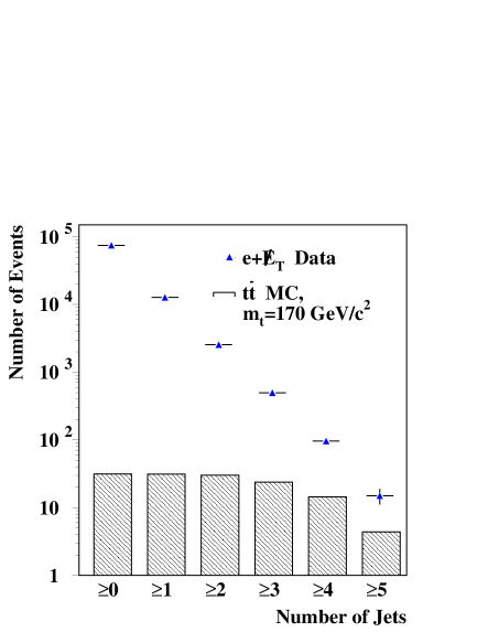
FIG. 14.: Jet multiplicity distribution for $e+{\mbox{$E\kern-5.70007pt\raise 0.81805pt\hbox{/}_{T}$}}$+jets data (triangle points) and $t\bar{t}$ Monte Carlo (hatched histogram) after initial selection. Trigger inefficiency is not included in the Monte Carlo samples.

Figure 14 shows the number of events as a function of the number of jets in the event for $e+$jets inclusive data and for $t\bar{t}$ MC events after the initial selection. As can be seen, the signal to background ratio is still very low. It is, therefore, necessary to further exploit the differences between signal and background. The most obvious differences are in the event topology and the presence or absence of a $b$ quark jet. The $b$ quark is inferred in the DØ detector by the presence of a non-isolated muon (muon tag). Therefore, two orthogonal analyses are employed beyond this point: (1) a purely topological analysis, which by construction does not contain a muon tag, and (2) an analysis that relies primarily on the presence of a muon tag, but also makes use of some topological cuts. These channels are denoted respectively as $\ell$+jets/topo and $\ell$+jets/$\mu$. The initial selection for these channels is given in Table 18.

FIG. 15.: Results of the random grid search in terms of expected signal vs expected background for the $e$+jets topological analysis for four possible variable sets: (a) ${\cal A}(W+{\rm jets})$ and $h$, (b) ${\cal A}(W+{\rm jets})$, $h$, and $\hbox to0.0pt{\kern 2.5pt/\hss}E_{T}$, (c) ${\cal A}(W+{\rm jets})$, $H_{T}$, and $\hbox to0.0pt{\kern 2.5pt/\hss}E_{T}$, (d) ${\cal A}(W+{\rm jets})$, $H_{T}$, and $p_{T}(W)$. See text for definitions of these variables.

In order to obtain the most precise measurement of the $t\bar{t}$ production cross section possible, an optimization was performed to find those topological variables that provide the best separation between signal and background. This was accomplished through the use of a random grid search [91] in which many possible cut points were tested on the signal and background models. Many variables were investigated in this way: $p_{T}(W)\equiv|\vec{p}_{T}^{W}|$, $\hbox to0.0pt{\kern 2.5pt/\hss}E_{T}$, $N_{\rm jets}$, $h\equiv\frac{E_{T}({\rm lepton})+E_{T}\!\!\!\!\!\!\!/}{H_{T}({\rm jets})+p_{T}(W)}$, two types of aplanarity ($\cal A$), and two types of $H_{T}$. Aplanarity is essentially a measure of the “flatness” of an event and is defined to be ${3\over 2}$ of the smallest eigenvalue of the normalized laboratory momentum tensor $({\cal M})$, where this tensor is defined by [92]

$${\cal M}_{ij}=\Bigl{(}\sum_{o}p_{o,i}p_{o,j}\Bigr{)}/\Bigl{(}\sum_{o}|\vec{p}_{o}|^{2}\Bigr{)},$$ (29)

where $\vec{p}_{o}$ is the three momentum of object $o$, $i,j$ correspond to the $x,y,$ and $z$ coordinates, and the objects included in the sum depend on the type of aplanarity under consideration: (1) only the jets, ${\cal A}({\rm jets})$, and (2) the jets and the reconstructed leptonic $W$, ${\cal A}(W+{\rm jets})$. Large values of ${\cal A}$ are indicative of spherical events, whereas small values correspond to more planar events. Events due to $t\bar{t}$ production are quite symmetric as is typical for the decay of a heavy object. $W$+jet and QCD multijet events are more planar, owing primarily to the fact that the jets in these events arise from gluon radiation.

Analogous to the transverse-energy variable defined for the $ee$ and $e\mu$ channels, and identical in form to that used for the $\mu\mu$ channel (see Eq. 19), $H_{T}$ is defined for the lepton+jets channels as

$$H_{T}\equiv\sum_{\rm jets}E_{T}.$$ (30)

The sum is over all jets with $E_{T}\geq 15$ GeV and $|\eta|\leq 2.0$ (recall that the $\mu\mu$ channel uses $|\eta|\leq 2.5$). The second transverse-energy variable is simply the sum of the standard $H_{T}$ and the magnitude of the $W$ boson transverse momentum vector, $H_{T}({\rm all})\equiv H_{T}+p_{T}(W)$. Events due to $t\bar{t}$ production tend to have much higher values of $H_{T}$ than background. This is due to the fact that the jet $E_{T}$ is typically much harder for jets originating from the decay of a heavy object than are those from gluon radiation.

The $t\bar{t}$ sample used in the optimization of all four channels is generated using herwig with $m_{t}=180$ $\mbox{GeV}/c^{2}$. The appropriate combination of $W$+jets and QCD multijet events is used for background. The $Z\rightarrow\mu\mu$ background to the $\mu$+jets/$\mu$ channel is not included in the optimization. For the $\ell$+jets/$\mu$ channels, both the $W$+jets and QCD multijet background estimates are based entirely on data. For the topological channels, the QCD multijet background is based on data and the $W$+jets contribution is modeled using the vecbos Monte Carlo. These background samples are used to investigate the region of phase space remaining after the initial selection (see Table 18), and thus differ somewhat from the samples used in the full background determination to be discussed in Secs. VII A and VII B.

FIG. 16.: Expected signal vs expected background plots for ${\cal A}(W+{\rm jets})$ and $H_{T}$ optimization variables for (a) $\mu$+jets/topo and (b) $e$+jets/$\mu$. The solid curves are contours of constant uncertainty on the cross section ($d\sigma/\sigma$). Arrows indicate chosen cut points.

All of these variables are studied in pairs and in different combinations, and for each set of cut points a corresponding point in the expected ($S$(signal),$B$(background)) plane is found. When all such points are plotted, they define a boundary that maximizes the expected signal for a given background level, which is termed the “optimal boundary” (see, for example, Fig. 15). Comparison of the optimal boundaries for the various combinations of variables shows that the pair ${\cal A}(W+{\rm jets})$ and $H_{T}$ provides the best signal to background ratio for a given signal efficiency.

After determining that ${\cal A}(W+{\rm jets})$ and $H_{T}$ are the best variables, it is necessary to select which cut point (on the optimal boundary) results in the most precise cross section measurement. Contours of constant uncertainty on the measured cross section ($d\sigma/\sigma$) can be derived from the relation

$$\sigma=\frac{S}{\varepsilon\cdot{\cal L}}=\frac{N-B}{\varepsilon\cdot{\cal L}}$$ (31)

where $N$, $S$, and $B$ are the number of observed, expected signal, and expected background events, respectively, $\varepsilon$ is the signal efficiency, ${\cal L}$ is the integrated luminosity, and $\sigma$ is the measured cross section [93]. The cut points on the optimal boundary with the smallest $d\sigma/\sigma$ and best significance ($s/b$) are (see Fig. 16):

$\ell$+jets/topo:

• $H_{T}\geq 180$ GeV

• ${\cal A}(W+{\rm jets})\geq 0.065$

$\ell$+jets/$\mu$:

• $H_{T}\geq 110$ GeV

• ${\cal A}(W+{\rm jets})\geq 0.040$.

Following the initial selection and optimization it is necessary to make several additional channel-specific requirements. These requirements, along with the results and expectations from signal and background, are discussed in the next two sections (VII A and VII B).

Acceptances for all four $\ell+$jets channels are computed from Monte Carlo events generated by the herwig [56] program for 24 top quark mass values ($m_{t}$ = 90–230 GeV/$c^{2}$) and then passed through the full DØ detector simulation (see Sec. V). The expected number of $t\bar{t}$ events passing the selection for a given channel is

$$N=\sigma_{t\bar{t}}(m_{t})\sum_{i={\rm runs}}\sum_{j={\rm det}}A(i,j,m_{t})\cdot{\mathcal{L}}_{i,j}$$ (32)

where $\sigma_{t\bar{t}}(m_{t})$ is the theoretical $t\bar{t}$ cross section at a top quark mass of $m_{t}$ [47]; ${\mathcal{L}}_{i,j}$ is the integrated luminosity for run $i$ and detector region $j$ (CC and EC for electrons, CF and EF for muons); and the acceptance is

$$A(i,j,m_{t})=\varepsilon_{\rm trig}\cdot\varepsilon_{\rm pid}\cdot\varepsilon_{\rm sel}\cdot G\cdot{\cal B},$$ (33)

where $\varepsilon_{\rm trig}(i,j,m_{t})$ is the trigger efficiency, $\varepsilon_{\rm pid}(i,j)$ is the efficiency for lepton identification (isolated leptons and muon tag), $\varepsilon_{\rm sel}(i,j,m_{t})$ is the efficiency of the selection cuts, $G(i,j)$ is the geometrical acceptance, and ${\cal B}$ is the branching fraction for the sample in question. Trigger efficiencies are obtained from data or Monte Carlo events, depending on the channel, and are discussed in more detail below. Particle identification efficiencies are obtained from data for the case of electrons (as discussed in Sec. IV A) and from a combination of data and Monte Carlo in the case of muons (as discussed in Sec. IV B). The selection efficiencies $\varepsilon_{\rm sel}$ and the geometrical acceptances $G$ are obtained from Monte Carlo events. As discussed in Sec. X, the acceptance, rather than the expected number of $t\bar{t}$ events, is used in the calculation of the $t\bar{t}$ cross section. Typical values for the acceptance, often denoted as the “efficiency times branching fraction” ($\varepsilon\times{\cal B}$), for all eight leptonic channels, are given in Sec X for seven top quark masses. The numbers of $t\bar{t}$ events expected in the four $\ell+$jets channels are given in Tables 22 and 25 Secs VII A and VII B for the same set of top quark masses. The systematic uncertainties on the acceptances and backgrounds are discussed in Sec. IX.

A Topological tag

As described in the previous section, the first two stages of the $\ell$+jets/topo selection require the cuts described in Table 18 followed by the cuts on ${\cal A}(W+{\rm jets})$ and $H_{T}$. There is, however, one cut in Table 18 which has not yet been discussed. This cut on $\eta(W)$, the pseudorapidity of the lepton and $E\kern-5.70007pt\raise 0.81805pt\hbox{/}_{T}$ fit to a $W$ boson hypothesis, is designed to remove from consideration those regions of phase space where the $W$+jets vecbos Monte Carlo does not model the $W$+jets data very well. As can be seen in Fig. 17, the vecbos prediction is considerably below the data in the forward region [94]. Therefore, the initial selection requires that $|\eta(W)|\leq 2.0$. It should be noted that only a few percent of $t\bar{t}$ events have $|\eta(W)|>2.0$, so this cut does not represent a serious reduction in acceptance. It should further be noted that these analyses determine the $W$+jets backgrounds primarily from the data. The vecbos Monte Carlo is only used to determine the survival probability for the cuts on ${\cal A}(W+{\rm jets})$, $H_{T}$, and $E_{T}^{L}$ which is the scalar sum of the lepton $E_{T}$ and $E\kern-5.70007pt\raise 0.81805pt\hbox{/}_{T}$. As can be seen in Fig. 18, a requirement of $E_{T}^{L}\geq 60$ GeV provides significant rejection against QCD multijet background while having little effect on the $t\bar{t}$ signal.

FIG. 17.: $|\eta(W)|$ distribution for $\ell$+jets/topo data (histogram) for the sum of predicted signal and background (filled circles), and background alone (open triangles), after application of all selection criteria except the $\eta(W)$ cut.

         

FIG. 18.: $E_{T}^{L}$ distributions for $t\bar{t}$ Monte Carlo ($m_{t}=170$ GeV/$c^{2}$) (dashed histogram), and for QCD multijet data (solid histogram), after application of all selection criteria except those on $E_{T}^{L}$, ${\cal A}$, and $H_{T}$. The distribution for $W$+jets is similar to that for $t\bar{t}$. The solid vertical line at $E_{T}^{L}=60$ GeV indicates the cutoff value.

As noted above, the primary backgrounds to the $\ell$+jets/topo channels are from $W(\rightarrow\ell\nu)$+jets and QCD multijet events which contain a misidentified electron or isolated muon and mismeasured $E\kern-5.70007pt\raise 0.81805pt\hbox{/}_{T}$. The mismeasured $E\kern-5.70007pt\raise 0.81805pt\hbox{/}_{T}$ arises primarily from mismeasurement of jet $E_{T}$ or vertex $z$ position.

The background calculation proceeds in four steps:

1. The QCD multijet background is determined as a function of the inclusive jet multiplicity from data samples in which the ${\cal A},H_{T},\eta(W)$, and $E_{T}^{L}$ cuts have not been applied. Due to the different processes that give rise to a misidentified electron or isolated muon, these backgrounds are handled differently:

   • Jets that have a large electromagnetic fraction can sometimes pass the electron identification criteria and be misidentified as electrons. To determine the background from multijet events containing such misidentified electrons and $E\kern-5.70007pt\raise 0.81805pt\hbox{/}_{T}$, one begins with the $E\kern-5.70007pt\raise 0.81805pt\hbox{/}_{T}$ spectrum from $n+1$ jet ($n\geq 0$) events with $|\eta(W)|\leq 2.0$ which pass an electron trigger but fail the full electron identification cuts (mis-id $e$ + $E\kern-5.70007pt\raise 0.81805pt\hbox{/}_{T}$ sample). This sample correctly describes (with sufficient statistics) the $E\kern-5.70007pt\raise 0.81805pt\hbox{/}_{T}$ distribution for the QCD multijet background, but the normalization is not correct since the electron identification requirement has not been made. The correct normalization is obtained by matching the number of events at low $E\kern-5.70007pt\raise 0.81805pt\hbox{/}_{T}$ (${\mbox{$E\kern-5.70007pt\raise 0.81805pt\hbox{/}_{T}$}}\leq 10$ GeV) to that found in a complementary sample that passes the normal electron identification criteria. Requiring ${\mbox{$E\kern-5.70007pt\raise 0.81805pt\hbox{/}_{T}$}}\geq 25$ GeV then provides the expected number of QCD multijet background events to the $e+n$ jet selection. Uncertainties on this procedure are dominated by the statistics of the samples used and range from 9.5% (13%) for the Run 1a (Run 1b) $e+1$ jet selection to 27% (54%) for the Run 1a (Run 1b) $e+4$ jet selection.

   • Muons from the semi-leptonic decay of a $b$ or $c$ quark are normally accompanied by an associated jet (non-isolated). However, occasionally the decay kinematics are such that there is insufficient hadronic energy to produce a jet. In these cases the muons from semi-leptonic $b$ and $c$ decays will appear to be isolated. The probability that a muon originating from the decay of a heavy quark will appear isolated varies with jet multiplicity, run period, and detector region, and is denoted by $I_{\rm mis-id}({\rm run,det})$. Typical CF values are 11% for $\mu+\geq 1$ jet events and 6% for $\mu+\geq 2,\geq 3,\geq 4$ jet events (the corresponding EF values are 22% and 15% respectively). For a given jet multiplicity, $n$, these probabilities are measured using samples of QCD multijet events with ${\mbox{$E\kern-5.70007pt\raise 0.81805pt\hbox{/}_{T}$}}\leq 20$ GeV as the ratio of the number of isolated-$\mu$ + $\geq n$ jet events to the number of non-isolated-$\mu$ + ($\geq n+1$) jet events. The QCD multijet background is defined by the product of this probability and the number of non-isolated-$\mu$ + ($\geq n+1$) jet events with ${\mbox{$E\kern-5.70007pt\raise 0.81805pt\hbox{/}_{T}$}}>20$ GeV. The primary uncertainty in this method stems from the determination of the above misidentified muon isolation probabilities. The value of 30% assigned to this uncertainty is dominated by the statistical precision of the control sample used to derive the false isolation fraction for four-jet events.

   These procedures are carried out for each inclusive jet multiplicity, thereby providing the expected QCD multijet contribution to the $\ell+\geq n$ jet selections ($n$ = 1,2,3,4), as defined in Table 18. For the $\ell+\geq 4$ jet selection, the expectation is $4.4\pm 2.2$ events in the $e+$jets/topo channel and $6.44\pm 2.08$ in the $\mu+$jets/$mu$ channel.

2. The background from $W(\rightarrow\ell\nu)+$jets is computed by performing a fit to the jet-multiplicity spectrum that remains following the subtraction of the QCD multijet background. Inherent in the fit is the assumption of “Berends ($N_{\rm jets}$) scaling” [95, 96] which suggests that there is a simple exponential relationship between the number of events and the jet multiplicity:

   $$\frac{\sigma(W+n{\rm\ jets)}}{\sigma(W+(n-1){\rm\ jets})}=\alpha,$$ (34)

   where $\alpha$ is a constant (for any given jet $E_{T}$ and $\eta$ requirements) and $n$ is the inclusive jet multiplicity. For any given inclusive jet multiplicity $i$, the number of events which are observed following the QCD multijet subtraction is given by

   $$N_{i}^{\rm obs}=N_{1}^{W}\cdot\alpha^{i-1}+f_{i}^{\rm top}\cdot N^{\rm top},$$ (35)

   where $N_{1}^{W}$ is the number of $W+1$ jet events, $N^{\rm top}$ is the number of $t\bar{t}$ events in the sample, and $f_{i}^{\rm top}$ is the fraction of $t\bar{t}$ events with jet multiplicity $i$ (obtained from Monte Carlo). The values of $N_{i}^{\rm obs}$ are plotted in Fig. 19. Fits to Eq. 35 determine the values of $\alpha$ given in column 2 of Table 21 ($N_{1}^{W}$ and $N^{\rm top}$ are also obtained from this fit).

            

   FIG. 19.: Number of events as a function of inclusive jet multiplicity for the $e$+jets/topo and $\mu$+jets/topo analyses. All cuts have been applied except ${\cal A}$ and $H_{T}$. The linear nature of the distributions is known as Berends scaling. Note that since the $E_{T}^{L}$ cut has been applied, the values here differ from those in Table 20.

   TABLE 20.: Number of $\ell$+jets/topo data events passing at each cut level. Note that the $e$+jets luminosity of 90.9 ${\rm pb}^{-1}$ does not include recovered Main-Ring data (see Appendix C) – the Main-Ring contribution is given in parentheses. Similarly, the luminosity for the $\mu$+jets channel does not include Run 1a or recovered Main-Ring data. The Main-Ring contribution plus that from Run 1a is given in parentheses.

   
   

   	$e$+jets	$\mu$+jets
   Lum (${\rm pb}^{-1}$)	90.9	76.6
   $N_{\rm jets}\geq 1$	6604	2127
   $N_{\rm jets}\geq 2$	1225	537
   $N_{\rm jets}\geq 3$	223	124
   $N_{\rm jets}\geq 4$	39	28
   $E_{T}^{L}\geq 60$ GeV,	39	22
   ${\cal A}\geq 0.065$,	18	10
   $H_{T}\geq 180$ GeV	7(2)	4(6)

   TABLE 21.: Steps in $e$+jets/topo and $\mu$+jets/topo background calculation: column 2, row 1 gives the expected number of QCD multijet background events ($\ell$+4 jets); column 1, row 2 gives the value of $\alpha$ determined from the fit to Eq. 35; column 2, row 2 gives the expected number of $W$+4 jet events; column 3 gives the trigger and Main-Ring (MR) correction factors; column 4 gives the result of multiplying column 2 by column 3 (step 3 in the text); column 5 gives the $E_{T}^{L}$, ${\cal A}$, $H_{T}$ cut survival probabilities; and column 6 gives the final expected background obtained by multiplying column 4 by column 5. Note that Runs 1a and 1b are treated separately for the $e$+jets channel whereas they are treated as a single run for the $\mu$+jets channel.

   
   

   			Exp # of evts	Trigger &	Exp # of evts	$E_{T}^{L},{\cal A},H_{T}$ cut	Exp # evts
   		$\alpha$	Steps 1-2	MR corr	Step 3	survival prob. ($f$)	Step 4
   $e+$jets	QCD multijet 1a		$0.7\pm 0.8$	$1.09\pm 0.39$	$0.76\pm 0.91$	$0.071\pm 0.040$	$0.054\pm 0.072$
   	1b		$3.7\pm 2.0$	$1.71\pm 0.12$	$6.4\pm 2.0$	$0.051\pm 0.010$	$0.325\pm 0.119$
   	Total		$4.4\pm 2.2$	–	$7.16\pm 2.20$	–	$0.379\pm 0.139$
   	$W+$jets 1a	$0.17\pm 0.02$	$5.45\pm 1.53$	$1.09\pm 0.17$	$5.9\pm 1.9$	$0.092\pm 0.061$	$0.544\pm 0.185$
   	1b	$0.18\pm 0.01$	$31.77\pm 4.24$	$1.22\pm 0.06$	$38.9\pm 8.3$	$0.092\pm 0.061$	$3.590\pm 0.799$
   	Total		$37.21\pm 4.50$	–	$44.8\pm 8.6$	–	$4.135\pm 0.899$
   $\mu+$jets	QCD multijet		$6.44\pm 2.08$	–	$13.9\pm 4.4$	–	$0.993\pm 0.498$
   	$W+$jets	$0.19\pm 0.02$	$18.8\pm 3.2$	$1.37\pm 0.07$	$25.8\pm 4.6$	$0.129\pm 0.027$	$3.324\pm 0.911$

   Once $\alpha$ is known, the number of $W+4$ jet events that pass the initial selection can be determined from the equation

   $$N_{4}^{W}=N_{1}^{W}\cdot\alpha^{3}.$$ (36)

   The resulting $W$+jets background after the $\ell+4$ jet selection is $37.2\pm 4.5$ events for the $e+$jets channel and $18.8\pm 3.2$ events for the $\mu+$jets, as indicated in Table 21. This method, solely based on data, is independent of theoretical calculations of $W+n$ jet cross sections which have large uncertainties at high jet multiplicities.

3. For the $e+$jets channel only, a correction factor of $1.09\pm 0.39$ ($1.71\pm 0.12$) is applied to the Run 1a (Run 1b) QCD multijet background results to account for trigger differences between the background method and the actual data selection and for the increased luminosity from the inclusion of the Main-Ring data (see Sec. III and Appendix C) in the Run 1a and Run 1b data sets. A similar correction factor of $1.09\pm 0.17$ ($1.22\pm 0.06$) is applied to the Run 1a (Run 1b) $W+$jets background. Following these corrections, the backgrounds to the $e+4$ jets selection are found to be $7.2\pm 2.2$ events from QCD multijet and $44.8\pm 8.6$ events from $W+$jets.

4. To determine the expected background following the final three cuts on $E_{T}^{L}$, ${\cal A}$, and $H_{T}$ (see Table 21), a cut survival probability $f$ is computed for each background. This probability factor is applied to the results obtained after the $\ell+\geq 4$ jet selections, thus giving the final expected QCD multijet and $W+$jet backgrounds:

   $$N({\rm total\ bkg})=N^{\rm QCD}_{\ell+4j}\cdot f_{\rm QCD}+N^{W}_{\ell+4j}\cdot f_{W}$$ (37)

   where $N^{\rm QCD}_{\ell+4j}$ and $N^{W}_{\ell+4j}$ are the QCD multijet and $W+$jet background estimates following the $\ell+\geq 4$ jet selections, and $f_{\rm QCD}$ and $f_{W}$ are the survival probability factors for the QCD multijet and $W+$jets backgrounds respectively.

   • For the $e+$jets channel, $f_{\rm QCD}$ is determined from the combined $E_{T}^{L}$, ${\cal A}$, and $H_{T}$ pass rate on a sample of misidentified electron+4 jet events that satisfy the $E\kern-5.70007pt\raise 0.81805pt\hbox{/}_{T}$ and $\eta(W)$ requirements.

   • For the $\mu+$jets channel, the prescription is simply an extension of the QCD multijet background computation described above for the $\mu+n$ jet selection. Specifically, the selection criteria are applied to five-jet events, where the jet associated with the non-isolated muon is not included in the ${\cal A}$ and $H_{T}$ calculations.

   For both channels, $f_{W}$ is determined using the vecbos Monte Carlo program to measure the final efficiency (including the $\ell+\geq 4$ jet, $E_{T}^{L}$, ${\cal A}$, and $H_{T}$ cuts) relative to that for the $\ell+\geq 4$ jet selection. To investigate the systematic uncertainties associated with this Monte Carlo based procedure, samples are generated with two different $Q^{2}$ scales, $M_{W}^{2}$ and $\left<p_{T}^{2}({\rm jet})\right>$, and with two different hadronic fragmentation prescriptions, isajet and herwig. Comparison with the background-enriched sample of data indicates that vecbos generated at $Q^{2}=\left<p_{T}^{2}({\rm jet})\right>$ and fragmented through herwig provides the best match. This choice is therefore used to compute the values of $f_{W}$.

These four steps are summarized in Table 21.

TABLE 22.: Observed and expected number of $\ell$+jets/topo signal and background events after all cuts. Uncertainties shown are statistical and systematic contributions added in quadrature. The total background systematic uncertainty includes correlations among the different background sources.

	$e$+jets	$\mu$+jets
Lum (${\rm pb}^{-1}$)	119.5	107.7
Observed	9	10
top MC $m_{t}$ (GeV/$c^{2}$)
140	$12.06\pm 5.20$	$8.22\pm 3.56$
150	$11.20\pm 3.72$	$7.83\pm 2.98$
160	$10.11\pm 2.35$	$7.12\pm 2.40$
170	$8.97\pm 1.61$	$5.72\pm 1.72$
180	$7.44\pm 1.04$	$4.80\pm 1.27$
190	$5.70\pm 0.68$	$3.84\pm 0.92$
200	$4.60\pm 0.47$	$3.14\pm 0.69$
$W$+jets	$4.14\pm 0.90$	$3.32\pm 0.91$
QCD multijet	$0.38\pm 0.14$	$0.99\pm 0.50$
Total background	$4.51\pm 0.91$	$4.32\pm 1.04$

     

FIG. 20.: Scatter plots of ${\cal A}$ vs $H_{T}$ for $\ell+$jets data (d) compared to expectations from higher-luminosity samples of $t\bar{t}$ MC ($m_{t}$ = 170 $\mbox{GeV}/c^{2}$) (c), and QCD multijet (b) and $W+$4 jet MC (a) backgrounds. The dashed lines represent the threshold values used for selection. The effective luminosity given for plot (b) is determined as the product of the luminosity of the selected multi-jet sample and the inverse of the appropriate misidentification rate.

Figure 20 shows the distribution of ${\cal A}$ vs $H_{T}$ for $\ell+$jets (combined $e+$jets and $\mu+$jets) events for data, herwig $t\bar{t}$ Monte Carlo ($m_{t}$ = 170 $\mbox{GeV}/c^{2}$), QCD multijet, and vecbos $W+$jets Monte Carlo events. From this figure it is clear that ${\cal A}$ and $H_{T}$ provide significant discrimination between signal and background.

As described in Sec. VII, $t\bar{t}$ acceptances are computed via Eq. 33 using Monte Carlo events generated with herwig and passed through the DØ detector simulation. The trigger efficiency for the $e$+jets channel is obtained from $W$+jets data and determined to be $98.2^{+1.8}_{-4.4}$%. For the $\mu$+jets channel, the trigger efficiency is computed using data-derived trigger turn-on curves applied to $t\bar{t}$ Monte Carlo and is determined to be $89\pm 5$%. The acceptance values after all cuts for seven different top quark masses (and for all channels) are given in Sec. X.

Following Eq. 32, the expected numbers of $t\bar{t}$ events in the $\ell+$jets/topo channels are given in Table 22 for these same seven masses. Also shown are the final numbers of events observed in the data, 9 in the $e+$jets channel and 10 in the $\mu+$jets channel. Table 20 shows the observed number of data events passing at the different stages of the selection procedure. Note that for this table, the $e$+jets luminosity does not include Main-Ring data and the $\mu$+jets luminosity does not include Run 1a or Main-Ring data. Finally, the cross section obtained from the $e$+jets/topo and $\mu$+jets/topo channels are $2.8\pm 2.1$ pb and $5.6\pm 3.7$ pb, respectively.

B $\mu$ tag

The initial selection for $\ell+$jets/$\mu$ events is described in Sec. VII and summarized in Table 18. All events are required to have a $\mu$ tag as defined in Sec. IV B.

The dominant backgrounds that remain after the initial selection arise from $W(\rightarrow\ell\nu)$+jets production, QCD multijet events that contain a misidentified electron or isolated muon and mismeasured $E\kern-5.70007pt\raise 0.81805pt\hbox{/}_{T}$, and also $Z(\rightarrow\mu\mu)+$jets for the $\mu$+jets/$\mu$ channel.

For events that have no genuine source of $E\kern-5.70007pt\raise 0.81805pt\hbox{/}_{T}$, the presence of a muon, as a consequence of the muon system’s modest momentum resolution, may lead to mismeasured $E\kern-5.70007pt\raise 0.81805pt\hbox{/}_{T}$ which is aligned or anti-aligned with the muon $p_{T}$. Indeed, in multijet data, the distribution of the angle $\phi$ between the muon momentum and the direction of the $E\kern-5.70007pt\raise 0.81805pt\hbox{/}_{T}$, $\Delta\phi(\mu,{\mbox{$E\kern-5.70007pt\raise 0.81805pt\hbox{/}_{T}$}})$, peaks at $0^{\rm o}$ and $180^{\rm o}$, whereas for $t\bar{t}$ events this distribution rises monotonically from $0^{\rm o}$ to $180^{\rm o}$ as indicated in Fig. 21. In order to reduce background from QCD multijet events, both $\mu$-tag channels make a cut on the allowed region in the $E\kern-5.70007pt\raise 0.81805pt\hbox{/}_{T}$, $\Delta\phi(\mu,{\mbox{$E\kern-5.70007pt\raise 0.81805pt\hbox{/}_{T}$}})$ plane:

$$\mbox{$\hbox to0.0pt{\kern 2.5pt/\hss}E_{T}$}>35{\rm\ GeV,\ if\ \ }|\Delta\phi(\mu,{\mbox{$E\kern-5.70007pt\raise 0.81805pt\hbox{/}_{T}$}})|\leq 25^{\rm o},{\rm\ \ \ for\ }e+{\rm jets,}$$ (38)

and,

$$\Delta\phi(\mu,{\mbox{$E\kern-5.70007pt\raise 0.81805pt\hbox{/}_{T}$}}) < 170^{\rm o}{\rm\ \ \ \ \ \ \ \ \ and\ }$$ (39)

$$\frac{|\Delta\phi(\mu,{\mbox{$E\kern-5.70007pt\raise 0.81805pt\hbox{/}_{T}$}})-90^{\rm o}|}{90^{\rm o}} \leq \frac{{\mbox{$E\kern-5.70007pt\raise 0.81805pt\hbox{/}_{T}$}}}{45{\rm\ GeV}},{\rm\ \ \ for\ }\mu+{\rm jets}.$$ (40)

The effectiveness of these cuts is displayed in Fig. 21, which shows the distributions in the $E\kern-5.70007pt\raise 0.81805pt\hbox{/}_{T}$,$\Delta\phi(\mu,{\mbox{$E\kern-5.70007pt\raise 0.81805pt\hbox{/}_{T}$}})$ plane for QCD multijet events and $t\bar{t}$ Monte Carlo events for both $\mu$-tag channels.

      

FIG. 21.: Scatter plots of $\Delta\phi(\mu,\mbox{$\hbox to0.0pt{\kern 2.5pt/\hss}E_{T}$})$ vs $\hbox to0.0pt{\kern 2.5pt/\hss}E_{T}$ for (a) $e$+jets/$\mu$ QCD multijet background, (b) $t\bar{t}\rightarrow e+{\rm jets}/\mu$, (c) $\mu$+jets/$\mu$ QCD multijet background, and (d) $t\bar{t}\rightarrow\mu+{\rm jets}/\mu$. The solid lines define the cut boundaries.

In addition to the QCD multijet and $W+$jets backgrounds noted above, the $\mu$+jets/$\mu$ channel, by virtue of the fact that it requires two muons, has a non-negligible background from $Z(\rightarrow\mu\mu)+$jets production. Although the muons from $Z$ boson decay are, in principle, isolated, there is a small probability that one of them will overlap with one of the jets in the event and thus appear to be non-isolated. The $\mu$+jets/$\mu$ channel relies therefore on a kinematic fitting procedure to reduce this background. As described in Sec. VI C, a kinematic fit to the $Z\rightarrow\mu\mu$ hypothesis is performed and a $\chi^{2}$ is obtained (see Eqs. 25 and 27). Events with a $\chi^{2}$ probability greater than 1%, $P(\chi^{2})>0.01$, are considered likely $Z$ boson candidates and are therefore rejected. As can be seen in Fig. 22, this procedure provides very good rejection against the $Z(\rightarrow\mu\mu)+$jets background and has essentially no effect on the $t\bar{t}$ signal.

FIG. 22.: $\chi^{2}$ probability distribution for the $\mu+$jets/$\mu$ channel after all cuts except $P(\chi^{2})$: (a) $Z(\rightarrow\mu\mu)+$jets MC and (b) $t\bar{t}$ MC.

The general scheme for background calculation proceeds in three steps which are first outlined and then discussed in detail:

1. Compute the QCD multijet background:

   • For the $e+$jets/$\mu$ channel, the QCD multijet background is computed by applying an electron misidentification rate to a $\mu$-tagged multijet control sample passing all cuts except tight electron identification.

   • For the $\mu+$jets/$\mu$ channel, the QCD multijet background is computed by applying isolated-muon and muon-tag misidentification rates to an untagged QCD multijet control sample passing all other cuts except the isolated muon requirement.

2. Compute the $W+$jets background:
   For both channels, the background from $W+$jets events is computed by applying a muon tag rate to the number of untagged multijet-subtracted $\ell$ + $\geq 3$ jet data events and then subtracting the expectation from $t\bar{t}$:

   $$N_{W}({\rm bkg})=N({\rm data-QCD})\cdot P_{\rm tag}-N_{3}^{t\bar{t}}$$ (41)

   where
   “data” is the number of events passing all cuts except $\mu$-tag;
   “QCD” is
   (the number of (extra-loose-$e$+$\geq 3$ jet)/($\geq 4$ jet) events passing $\mbox{$\hbox to0.0pt{\kern 2.5pt/\hss}E_{T}$},{\cal A}$, and $H_{T}$ cuts) $\cdot$ ($e/\mu$ mis-id rate);
   “$P_{\rm tag}$” is the probability (as a function of jet $E_{T}$ and $\eta$, and run period) for a jet to contain a tagged muon, and is determined from QCD multijet data;
   “$N_{3}^{t\bar{t}}$” is the expected top quark contribution after all cuts and is computed differently for the $e+$jets/$\mu$ and $\mu+$jets/$\mu$ channels:

   • for the $e+$jets/$\mu$ channel, the expected top quark contribution is determined from data by fitting the jet spectra of the multijet-subtracted untagged $e+n$ jet data under the assumption of jet scaling and measuring the excess for $n\geq 3$. A tag rate derived from $t\bar{t}$ MC is applied to this excess to obtain $N_{3}^{t\bar{t}}$.

   • for the $\mu+$jets/$\mu$ channel, the expected top quark contribution ($N_{3}^{t\bar{t}}$) is determined from herwig MC normalized to the theoretical cross section [97].

3. For the $\mu$+jets/$\mu$ channel only, determine the background from $Z\rightarrow\mu\mu$ using vecbos MC events.

The key elements of this procedure, namely the QCD multijet background calculations and the parameterization of the muon-tagging probability, are motivated and developed below.

The estimation of the multijet background differs somewhat in the $e$+jets/$\mu$ and $\mu$+jets/$\mu$ channels. The calculation for the $e$+jets/$\mu$ channel is similar to that used for the $\ell$+jets/topo channels. Namely, the QCD multijet background is determined by relaxing the electron identification criteria and observing the number of additional events that pass the selection. It is assumed that the number of events in the extra-loose electron sample, $N_{l}$, consists of both real, $N_{e}$, and misidentified (often referred to as “fake”), $N_{f}$, electrons

$$N_{l}=N_{e}+N_{f}.$$ (42)

The probability for a real electron to pass from the loose sample into the tight sample, $\varepsilon_{t}^{e}$, is determined from $Z\rightarrow ee$ data. Similarly, the probability for a misidentified electron to make this transition, $\varepsilon_{t}^{f}$, is defined as the ratio of tight to loose electron events in a sample of “loose electron+1 jet” events without $\hbox to0.0pt{\kern 2.5pt/\hss}E_{T}$ [71]. These probabilities are determined separately for the CC and EC regions of the calorimeter and are given in Table 23. Applying these probabilities to the number of real and misidentified electrons in the loose sample gives the expected number of events in the tight sample:

$$N_{t}=\varepsilon_{t}^{e}N_{e}+\varepsilon_{t}^{f}N_{f}.$$ (43)

Eqs. 42 and  43 can be solved for the number of misidentified electron events in the loose sample:

$$N_{f}=\frac{\varepsilon_{t}^{e}N_{l}-N_{t}}{\varepsilon_{t}^{e}-\varepsilon_{t}^{f}}.$$ (44)

The expected number of misidentified electron events in the final sample is the product of the number in the loose sample and the probability for a misidentified electron to pass the tight requirement, $\varepsilon_{t}^{f}N_{f}$. Values for the CC and EC regions of the calorimeter are given in Table 23. The combined (CC+EC) QCD multijet background for the $e$+jets/$\mu$ channel, including additional systematic uncertainties (see Sec. IX) not given in Table 23, is tabulated later in this section.

TABLE 23.: $e$+jets/$\mu$ QCD multijet background calculation parameters

	CC	EC
$N_{t}$	4	1
$N_{l}$	8	6
$\varepsilon_{t}^{e}$	$0.828\pm 0.010$	$0.453\pm 0.015$
$\varepsilon_{t}^{f}$	$0.027\pm 0.009$	$0.053\pm 0.012$
$N_{f}$	$3.28\pm 0.11$	$4.30\pm 0.31$
$\varepsilon_{t}^{f}\cdot N_{f}$	$0.088\pm 0.030$	$0.228\pm 0.054$

The calculation of the QCD multijet background for the $\mu$+jets/$\mu$ channel is an extension of that used for the $\mu$+jets/topo channel. As described in Sec. VII A, the QCD multijet background calculation for the $\mu$+jets/topo analysis applied the probability for a muon from a $b$ or $c$ quark decay to appear isolated to the number of non-isolated-$\mu$+jet events to determine the expected number of misidentified isolated muon events in the signal sample. The $\mu$+jets/$\mu$ analysis extends this by applying an additional tag rate function. This tag rate function is based on a Monte Carlo sample containing a high fraction of $b$-quark jets, and is parameterized in terms of the jet $E_{T}$ as:

$$h(E_{T},{\rm run,det})=D({\rm run,det})\cdot{\rm tanh}\left(\frac{E_{T}-15.0{\rm\ GeV}}{40.0{\rm\ GeV}}\right)$$ (45)

where $D({\rm run,det})$ is a scale factor that depends on the run period and detector region under consideration. The QCD multijet background to the $\mu$+jets/$\mu$ channel is then determined from the product

$$N_{\rm QCD}=\\ \sum_{\rm run,det}\sum_{\rm jets}N_{0}\cdot I_{\rm mis-id}({\rm run,det})\cdot h(E_{T},{\rm run,det}),$$ (46)

where $N_{0}$ is the number of events which pass all selection criteria except for the isolation requirement on the high-$p_{T}$ $\mu$ and the $\mu$-tag requirement, and $I_{\rm mis-id}({\rm run,det})$ is the misidentified-isolated-$\mu$ probability discussed in Sec. VII A. The final value, including systematic uncertainties, is tabulated at the end of this section.

The jets produced in association with $W$ boson production originate primarily from final state gluon radiation. Therefore, except for a small contribution from gluon splitting ($g\rightarrow b\bar{b}$), $W+$jets events are expected to contain very few $b$ quarks and thus very few muon tags. In order to estimate this background, it is assumed that the heavy flavor ($b$ and $c$ quark) content in $W$+jets events is the same as in QCD multijet events [60]. The expected number of $W$+jets+$\mu$ tag events is therefore computed from the product of the number of untagged $W$+jet events and a muon-tag probability ($P_{\rm tag}$)

$$N_{W}({\rm tagged})=N_{W}({\rm not\ tagged})\cdot P_{\rm tag}.$$ (47)

This probability is defined in a control sample of multijet events by the fraction of jets that contain a muon within a cone of $\Delta R=0.5$ around a jet axis. The control sample consists of events collected with a multijet trigger (jet-multi, see Table 5) that have four or more jets reconstructed offline ($E_{T}\geq 15$ GeV, $|\eta|\leq 2$). These events were collected under essentially the same detector and accelerator conditions as the signal sample. The multijet and untagged $W$+jets samples have similar jet $E_{T}$ and $\eta$ distributions, and, since both samples owe their high jet multiplicity to gluon radiation, they should also have similar quark-flavor content.

     

FIG. 23.: Parameterization of the muon tag rate, for muons in the CF region from Run 1b, as a function of (a) jet $E_{T}$ and (b) jet $\eta$.

This fraction, also known as the tag rate, is parameterized explicitly as a function of jet $E_{T}$ and $\eta$, and is handled separately for the CF and EF regions of the muon system. The $\eta$ dependence is fit independently for the different run intervals used in the two analyses (see Table 19). The tag rate as a function of jet $E_{T}$ and $\eta$ for muons in the CF region for Run 1b is shown in Fig. 23. The tag rate increases with jet $E_{T}$ because higher-energy jets have, on average, higher energy muons that are more likely to penetrate the calorimeter and magnet and be detected. The shape of the $\eta$ distribution is primarily due to the geometrical acceptance of the muon system, but varies somewhat over the different run intervals. As a function of jet $E_{T}$, the data are fit to the functional form

$$f(E_{T})=\left\{\begin{array}[]{ll}A_{1}+A_{2}\,E_{T}+A_{3}\,E_{T}^{2},&\mbox{for $E_{T}\leq\rho$}\\ A_{1}+A_{2}\,\rho+A_{3}\,\rho^{2},&\mbox{for $E_{T}>\rho$}\end{array}\right.$$ (48)

where $\rho=-\frac{1}{2}A_{2}/A_{3}$, and the parameters $A_{1}$, $A_{2}$ and $A_{3}$ are free. The resulting curves for muons in the CF and EF regions are denoted $f^{\rm{CF}}$ and $f^{\rm{EF}}$ respectively. As a function of $\eta$, the data for muons in the CF region are fit to the functional form

$$g^{\rm{CF}}(\eta,r)=B_{1,r}\,(1+B_{4,r}\eta^{2})\,[ {\rm{erf}}(\eta B_{2,r}+B_{3,r})$$ (49)

$$-{\rm{erf}}(\eta B_{2,r}-B_{3,r})],$$ (50)

where $r$ labels the three periods of the run as specified in Sec. IV B, ${\rm{erf}}(x)=2/\sqrt{\pi}\int_{0}^{x}\exp(-t^{2})\,dt$, and the parameters $B_{1,r}$, $B_{2,r}$, $B_{3,r}$, and $B_{4,r}$ are free to vary. Similarly, for muons in the EF region, the data are fit to

$$g^{\rm{EF}}(\eta)=C_{1}\left\{\right. {\rm{erf}}[(|\eta|-C_{4})C_{2}+C_{3}]$$ (51)

$$\left.-{\rm{erf}}[(|\eta|-C_{4})C_{2}-C_{3}]\right\},$$ (52)

with free parameters $C_{1}$, $C_{2}$, $C_{3}$, and $C_{4}$. There is no run dependence in Eq. 51, since, as noted in Sec. IV B, the EF region of the muon system was only used during the final run period (Run 1b+c postclean). The complete tag rate function is

$$P_{\rm tag}(E_{T},\eta,r)= D^{\rm{CF}}_{r}\,f^{\rm{CF}}(E_{T})\,g^{\rm{CF}}(\eta,r)$$ (53)

$$+D^{\rm{EF}}_{r}\,f^{\rm{EF}}(E_{T})\,g^{\rm{EF}}(\eta),$$ (54)

where $D^{\rm{CF}}_{r}$ and $D^{\rm{EF}}_{r}$ are constants that normalize the predicted number of tagged jets in the control sample to the actual number. The values of the parameters in Eqs. 48–53 are given in Table 24.

TABLE 24.: $e$+jets+$\mu$ tag parameters from Eqs. 48 – 53.

$f$ Parameters			$g^{\rm{CF}}$ Parameters				$g^{\rm{EF}}$ Param.		Normalization Param.
	CF value	EF value		$r=1$	$r=2$	$r=3$		$r=3$		$r=1$	$r=2$	$r=3$
$A_{1}$	-0.243E-2	-0.902E-3	$B_{1,r}$	0.386E-2	0.363E-2	0.395E-2	$C_{1}$	0.349E-2	$D^{\rm{CF}}_{r}$	249.6	248.7	223.4
$A_{2}$	0.170E-3	0.847E-4	$B_{2,r}$	11.5	2.26	4.78	$C_{2}$	3.92	$D^{\rm{EF}}_{r}$			528.8
$A_{3}$	-0.397E-6	-0.368E-6	$B_{3,r}$	12.4	2.17	4.85	$C_{3}$	1.54
			$B_{4,r}$	-0.483	-0.477	-0.198	$C_{4}$	1.43

FIG. 24.: Tests of the muon tag rate. Shown are (Observed – Predicted)/Predicted values for data sets that originate from nine different triggers. Some of the scatter is due to statistics, as indicated by the horizontal error bars; the remainder is ascribed to systematic effects as described in Sec. IX A 16. The solid vertical line is the overall mean value and the dashed vertical lines are the uncertainty on the overall mean.

The accuracy of this procedure has been studied by comparing the predicted to observed number of events having a tagged jet for a variety of data samples representing different trigger conditions, physics processes, and jet multiplicities. These studies are summarized in Fig. 24, which shows the (Observed – Predicted)/Predicted values for data samples that originate from nine different triggers (see Table 5 for the definitions of these triggers):

• The inclusive multijet samples with minimum jet multiplicity of two, three, four, and five were taken with the triggers jet-min, jet-3-mon, jet-4-mon, and jet-multi, respectively. The last sample, with five jets selected offline, is a complete subset of the four jet sample used in the actual tag rate calculation, comprising about one-third of the jets in the control sample.

• The electron samples consist of events with a tight electron candidate, taken with the ele-1-mon (gis-dijet) trigger for the case of one (two) or more additional jets. Almost all of the “electrons” are false. The purpose of examining these events is to check for an excess of tags due to $b\overline{b}$ or $c\overline{c}$ production, where one heavy quark decays to an electron and the other to a muon. There is no evidence of such an excess, and none is expected because of the isolation and high $E_{T}$ requirements imposed on the electron.

• The photon samples consist of events with a tight photon candidate (see Sec. IV A), taken with the same triggers as the electron samples. About 30% of the $\gamma+\geq 1$ jet events are from direct-photon production and the rest are from multijet background [98]. The purity is less in the $\gamma+\geq 2$ jet data.

• The $Z+{\rm jet}$ data were obtained with the em1-eistrkcc-esc trigger, by requiring two loose electron candidates including at least one tight candidate. The invariant mass of the electron pair is required to be between 80 and 100 $\mbox{GeV}/c^{2}$. The background in this sample is low (10%); but unfortunately only four events with a tagged jet survive, so the statistical uncertainty is quite large.

The horizontal error bars shown in Fig. 24 reflect the statistical uncertainty on each comparison. As discussed in Sec. IX, that portion of the scatter that cannot be attributed to the statistical uncertainty is taken as a measure of the systematic uncertainty of the tag rate procedure.

The functional dependence of the tag rate is important only to the extent that the target sample differs from the control sample. It should therefore be noted that the test samples with low jet multiplicity have significantly steeper jet $E_{T}$ spectra than either the control sample or the $W+\rm{jets}$ data after application of the $\cal{A}$ and $H_{T}$ cuts.

Because these analyses are concerned with the number of tagged events that remain in a data sample following selection cuts on $H_{T}$ and $\cal{A}$, it is important to confirm that the tag rate does not depend on these variables in an unexpected way. Figure 25 shows a comparison of the predicted and observed numbers of tagged events as a function of $H_{T}$ and $\cal{A}$ for the $\geq 3$ jet and $\geq 4$ jet test samples. The aplanarity distributions are in good agreement. Differences in the $H_{T}$ distributions suggest that a cut could result in a discrepancy of a few percent between the predicted and observed number of events. This is among the contributors to the tag-rate uncertainty that are discussed in Sec. IX A 16.

As noted in the outline at the beginning of this section, contamination from QCD multijet and $t\bar{t}$ events requires that the background from $W+$jets be computed via Eq. 41. The QCD multijet contribution to the untagged sample is estimated by applying the lepton ($e$/$\mu$) misidentification rate to a sample of (loose-$e+\geq 3$ jet)/($\geq 4$ jet) events that have passed the $\mbox{$\hbox to0.0pt{\kern 2.5pt/\hss}E_{T}$},{\cal A}$, and $H_{T}$ requirements. The $t\bar{t}$ contribution ($N_{3}^{t\bar{t}}$) for the $e+$jets/$\mu$ channel is determined from data by fitting the jet spectra of the QCD-multijet-subtracted $e+n$ jet data under the assumption of jet scaling and measuring the excess for $n\geq 3$. Following the hypothesis of jet multiplicity scaling, the number of $W+$jet events can be described by a function of the form

$$n_{i}=n^{W}_{3}\alpha^{(i-3)}+n_{3}^{t\bar{t}}f_{i}/f_{3}$$ (55)

where $n_{i}$ is the number of events with $i$ or more jets, $n^{W}_{3}$ is the number of $W$ boson events with three or more jets, $f_{i}$ is the number of events in the $t\bar{t}$ MC sample with $i$ or more jets, and $\alpha$ is a free parameter. A fit to Eq. 55 finds $n_{3}^{t\bar{t}}$ to be $19.2\pm 9.5$ events. $N_{3}^{t\bar{t}}$ is determined by applying the $t\bar{t}$ tag rate ($P_{\rm tag}^{t\bar{t}}$) to $n_{3}^{t\bar{t}}$. The $t\bar{t}$ contribution ($N_{3}^{t\bar{t}}$) for the $\mu+$jets/$\mu$ channel is determined from herwig MC normalized to the theoretical cross section [97].

As given in Table 25, the $W$+jets backgrounds for the $e$+jets/$\mu$ and $\mu$+jets/$\mu$ channels are determined via the multi-step procedure above to be $0.74\pm 0.30$ and $0.73\pm 0.14$ events respectively. Systematic uncertainties on the $W$+jets background arise primarily from uncertainties in Berends scaling and $t\bar{t}$ MC tag rate ($e+$jets/$\mu$ channel only) and the tag-rate parameterization. These are discussed in Sec. IX.

The background from $Z\rightarrow\mu\mu$ to the $\mu$+jets/$\mu$ channel is determined from vecbos $Z+$jets Monte Carlo events in a fashion similar to the Monte Carlo background calculations used for the dilepton channels (see Eq. 22) and is given in Table 25.

       

FIG. 25.: Predicted (histogram) and observed (filled circles) $H_{T}$ and $\cal{A}$ distributions in multijet data: (a) $H_{T}$ distributions for $\geq 3$ jet data, (b) $\cal{A}$ distributions for $\geq 3$ jet data, (c) $H_{T}$ distributions for $\geq 4$ jet data, and (d) $\cal{A}$ distributions for $\geq 4$ jet data.

Backgrounds from single top, $WW$, and $WZ$ production were also studied and found to have a negligible contribution to the total combined background, and therefore are not included in this discussion.

TABLE 25.: Total observed and expected number of $\ell$+jets/$\mu$ events after all cuts.

	$e$+jets/$\mu$	$\mu$+jets/$\mu$
Lum (${\rm pb}^{-1}$)	112.6	108.0
Observed	5	6
$t\bar{t}$ MC $m_{t}$ ($\mbox{GeV}/c^{2}$)
140	$6.93\pm 1.35$	$4.65\pm 1.19$
150	$6.18\pm 1.06$	$3.31\pm 0.83$
160	$4.51\pm 0.73$	$2.60\pm 0.63$
170	$3.73\pm 0.57$	$2.34\pm 0.55$
180	$3.11\pm 0.46$	$1.84\pm 0.43$
190	$2.44\pm 0.36$	$1.40\pm 0.32$
200	$1.83\pm 0.27$	$1.08\pm 0.25$
$W$+jets	$0.74\pm 0.30$	$0.73\pm 0.14$
QCD multijet	$0.32\pm 0.26$	$0.50\pm 0.17$
$Z\rightarrow\mu\mu$	–	$0.17\pm 0.08$
Total background	$1.05\pm 0.40$	$1.40\pm 0.23$

The inclusive jet multiplicity spectrum of the $\ell$+jets/$\mu$ data obtained prior to enforcing the ${\cal A}$ and $H_{T}$ requirements is compared with that for the expected background in Fig. 26. Good agreement is seen in the background-dominated 1 and 2 jet bins, but for 3 or more jets, the excess due to $t\bar{t}$ production is evident in both $\mu$-tagged channels.

FIG. 26.: Inclusive jet multiplicity spectra for $\ell+$jets/$\mu$ data (circles) and expected background (triangles) obtained prior to applying the $\cal{A}$ and $H_{T}$ requirements. Note that good agreement is seen for the $\geq 1$ and $\geq 2$ jet bins, but the $\geq 3$ jet bin shows a clear excess in the data.

      

FIG. 27.: Scatter plots of $\cal{A}$ vs $H_{T}$ for the $e+$jets/$\mu$ channel for (a) vecbos $W+$jets MC background, (b) QCD multijet background, (c) herwig $t\bar{t}$ MC events ($m_{t}$ = 170 $\mbox{GeV}/c^{2}$), and (d) data.

      

FIG. 28.: Scatter plots of $\cal{A}$ vs $H_{T}$ for the $\mu$+jets/$\mu$ channel for (a) vecbos $W+$jets MC background, (b) QCD multijet background, (c) herwig $t\bar{t}$ MC ($m_{t}$ = 170 $\mbox{GeV}/c^{2}$), and (d) data. The effective luminosity given for plot (b) is determined as the product of the luminosity of the selected multi-jet sample and the inverse of the muon misidentification rate.

Figures 27 and 28 show the distributions of ${\cal A}$ vs $H_{T}$ for $e$+jets/$\mu$ and $\mu$+jets/$\mu$ events for data, herwig $t\bar{t}$ Monte Carlo ($m_{t}$ = 170 $\mbox{GeV}/c^{2}$), QCD multijet data, and vecbos $W+$jets Monte Carlo events. From these figures it is clear that the cuts on ${\cal A}$ and $H_{T}$ provide a significant improvement in the discrimination between signal and background for these channels.

As described in Sec. VII, the $t\bar{t}$ acceptances are computed via Eq. 33 using Monte Carlo events generated with herwig and passed through the DØ detector simulation. The trigger efficiency for the $e$+jets/$\mu$ channel is obtained from the Trigger Simulator (see Sec. V) and has been compared with that found for $W$+jets data to estimate its systematic error, resulting in a value of $99^{+1}_{-5}\%$. For the $\mu$+jets/$\mu$ channel, the trigger efficiency is computed in the same fashion as for the $\mu$+jets/topo channel using data-derived trigger turn-on curves applied to $t\bar{t}$ Monte Carlo events and is determined to be $96^{+4}_{-5}$ %. The acceptance values after all cuts for seven different top quark masses (and for all channels) are given in Sec. X (Table 32). Following Eq. 32, the expected number of $t\bar{t}$ events in the $\ell$+jets/$\mu$ channels are given in Table 25 for these same seven masses. Also shown in Table 25 are the final numbers of events observed in the data, 5 in the $e$+jets/$\mu$ channel and 6 in the $\mu$+jets/$\mu$ channel. Finally, the cross section obtained from the $e$+jets/$\mu$ and $\mu$+jets/$\mu$ channels are $6.0\pm 3.6$ pb and $11.3\pm 6.6$ pb, respectively.

VIII Analysis of all-jets events

As noted in Sec. I, the all-jets channel is discussed in detail in Ref. [58] and is only summarized here.

The signature for the all-jets channel is characterized by the presence of six or more high transverse momentum jets. Given the overwhelming nature of the background to this channel, primarily from QCD multijet production, the challenge of this analysis is to develop selection criteria that provide maximum discrimination between signal and background, together with an estimate of the residual background in the signal region. Several kinematic and topological properties of the events were investigated, and neural networks employed to properly combine all possible sources of discrimination between signal and background. In order to improve the signal to background ratio, the analysis requires the presence of at least one muon-tagged jet in every event. Because the data provide an almost pure sample of background events, the background model is determined entirely from data. The modeling uses untagged events that are made to represent tagged events by adding muon tags to one of the jets in the event. The cross section is determined using fits to the neural network output, and checked using a conventional counting method. The cross section obtained for $m_{t}=172.1$ $\mbox{GeV}/c^{2}$is:

$$\sigma_{t\bar{t}}=7.3\pm 2.8({\rm stat})\pm 1.5({\rm sys}){\rm\ pb}.$$ (56)

This cross section differs slightly from the value reported in Ref. [58] due to an update of the luminosity normalization. The significance of the excess of $t\bar{t}$ signal over background is estimated by defining the probability $P$ of having the expected background fluctuate up to the observed number of events. This corresponds to a $3.2$ standard deviation effect, sufficient to establish the existence of a $t\bar{t}$ signal in multijet final states [58, 99].

IX Systematic uncertainties

The individual uncertainties which affect the acceptance and background are discussed below. A discussion of the treatment of the correlations between the uncertainties can be found in Appendix E.

A Sources

1 Luminosity

As noted in Sec. III, the luminosity is determined with the level 0 hodoscopes and is normalized to a world average total $p\bar{p}$ inelastic cross section from CDF [63], E710 [64], and E811 [65] Collaborations. The systematic uncertainty on the luminosity stems from both the level 0 measurement and the world average total $p\bar{p}$ inelastic cross section and is found to be 4.3%.

2 Energy scale

Uncertainty in the jet energy scale affects the cross section determination only via the uncertainty in the relative scale between data and MC. This uncertainty is determined by comparing $Z(\rightarrow ee){\rm+jet}$ events in data and MC [100]. Events are selected by requiring two electrons with $E_{T}\geq 15$ GeV, $82\ \mbox{$\mbox{GeV}/c^{2}$~{}}<m_{ee}<102\ \mbox{$\mbox{GeV}/c^{2}$}$, and at least one jet with $E_{T}\geq$ 15 GeV. The azimuthal bisector of the two electrons is determined and the transverse momentum of the $Z$ boson is projected along this bisector using the electron momentum vectors. The jet transverse momenta are also projected along this bisector with the contribution from each jet in the event summed to form the jet projection. The jet energy projection versus the $Z\rightarrow ee$ projection is plotted for MC (herwig and vecbos) and data from Run 1b, and a linear regression fit performed to determine the slope and offset of each sample. Comparison of the ratios of the slopes (MC/Data) and the differences in the offsets (MC – Data) indicate an uncertainty in the jet energy scale slope of 4% and an uncertainty in the jet energy scale offset of 1 GeV.

3 Electron identification

The procedure for determining the electron identification efficiencies is discussed in Sec. IV A 9. The primary source of uncertainty in this technique stems from the method used to subtract the background under the $Z$ boson mass peak. Comparison of several different background subtraction schemes [70] is used to determine the systematic uncertainties given in Table 6.

4 High $p_{T}$ and tag muon identification

As described in Sec. IV B 6, the muon identification efficiencies are determined from a modified version of døgeant which has additional corrections to account for time dependent detector inefficiencies and incorrect modeling of the muon track finding efficiency. The time dependent correction is applied only to Run 1a and Run 1b(preclean) with an uncertainty of 5%, arising primarily from statistical considerations. The track finding efficiency correction varied with detector region with an uncertainty of 1.5% in the CF and 2.2% in the EF, also arising primarily from statistical considerations. The uncertainty arising from the detector simulation is determined by comparing $Z\rightarrow\mu\mu$ MC events which are passed through the modified version of døgeant with $Z\rightarrow\mu\mu$ data, the difference being a measure of the uncertainty. This uncertainty varies with run period, detector region, and muon identification choice, and includes uncertainties from the muon trigger efficiency. The uncertainties noted above are added in quadrature to determine the systematic uncertainty on the efficiencies given in Tables 7–9.

5 $e$+jets trigger

This uncertainty accounts for systematic variations in the trigger efficiency for those signal and background MC samples that rely primarily on electron triggers (see Table 1). The determinations of the trigger efficiencies for each channel are discussed in the subsections of Secs. VI and  VII. For electron trigger efficiencies determined via the Trigger Simulator ($e\mu$: signal and all MC backgrounds; $e\nu$: signal and all MC backgrounds; $e+$jets/$\mu$: signal), the systematic uncertainty is determined by comparing the trigger efficiency of $e+$jet data events (obtained from an unbiased trigger) with that found passing $W(\rightarrow e\nu)+$jet MC events through the Trigger Simulator. For electron trigger efficiencies determined directly from data: for the $ee$ channel, comparison of the $Z(\rightarrow ee)+$jets trigger rate obtained from unbiased data with that obtained from passing $Z(\rightarrow ee)+$jet MC through the Trigger Simulator found a difference of 1% which was taken as a measure of the uncertainty; for the $e+$jets channel, studies of the efficiency variation using different samples and cuts led to the assignment of an uncertainty of 3%.

6 $\hbox to0.0pt{\kern 2.5pt/\hss}E_{T}$+jets trigger

This uncertainty accounts for systematic variations in the efficiency of the $E\kern-5.70007pt\raise 0.81805pt\hbox{/}_{T}$ triggers (see Table 4). Trigger efficiencies from the $E\kern-5.70007pt\raise 0.81805pt\hbox{/}_{T}$ triggers were obtained from measured turn-on curves convoluted with kinematics from MC events. The systematic uncertainty is determined from the differences in efficiency due to variations in top quark mass (for signal) and variations in the $\cal{A}$ and $H_{T}$ of the events (background). Note that efficiencies for the muon triggers were determined from a parameterization of the turn-on curves of the muon+jet triggers and the systematics have been folded into the uncertainty on the muon identification efficiency.

7 Multiple interactions

As discussed in Sec. III, there were, on average, 1.3 $p\bar{p}$ interactions per bunch crossing during Run 1, giving rise to additional minimum bias events produced along with the high-$p_{T}$ interactions of interest to the present analyses. These additional minimum bias events were not included in the MC models although they can contribute to mismeasurement of the primary interaction vertex and thus to mismeasurement of lepton and jet transverse energies/momenta. For $\ell+$jet events, such effects were found to be negligible since the presence of three or more hard jets from a single interaction vertex minimized any potential confusion in determining the correct vertex. For the dilepton channels the effect is more pronounced, and a systematic uncertainty is estimated for all signal and MC-based backgrounds. To make this estimate, additional signal and background MC samples were produced with one and two minimum bias events added. The efficiencies and background predictions from these samples are then weighted according to the luminosity distribution of the Run 1 data set and compared to the samples for which no minimum bias events had been added. The deviations, which vary significantly from channel to channel and between signal and background, are taken as an estimate of the uncertainty.

8 $t\bar{t}$ Monte Carlo generator (kinematics)

The uncertainty on the modeling of kinematic quantities (high-$p_{T}$ leptons, jets, and $\hbox to0.0pt{\kern 2.5pt/\hss}E_{T}$) due to imperfections in the MC generator is based on efficiency differences between the herwig and isajet generators. This uncertainty is calculated separately for each channel. The procedure, which is the same for each channel, is to generate a smooth curve summarizing the observed generator difference (isajet–herwig/herwig) for top quark masses from 140 GeV/$c^{2}$ to 200 GeV/$c^{2}$, ignoring any $b$-tag or $b$-tag-veto cuts. As seen in Table 26, the dilepton channels are parameterized using a constant relative uncertainty and the lepton+jets channels are parameterized using an exponential function of the top quark mass. The aspect of the generator to which the kinematic acceptance is most sensitive is the parton showering. herwig has been shown to reproduce jet properties well at both the Tevatron [101] and LEP [102]. Reference [101] describes a study of the topological properties (spectra of angles and energy distribution among jets) in inclusive three and four jet events and the authors find that “[a]part from the cos($\theta^{*}$) distributions, the herwig event generator provides a reasonably good description of the data while the differences between the data and the predictions of [the] isajet and pythia event generators are large in many distributions.”

TABLE 26.: Smoothed kinematic generator uncertainties for the eight leptonic channels.

Channel	Relative Uncertainty
	Fit	Applied
$ee$	5.5%	5%
$e\mu$	-4.9%	5%
$\mu\mu$	3.3%	5%
$e\nu$	-11.1%	12%
$e+{\rm jets}$	$\hbox{exp}(4.59-0.0407m_{t})$
$\mu+{\rm jets}$	$\hbox{exp}(0.546-0.0120m_{t})$
$e+{\rm jets}/\mu$	$\hbox{exp}(-0.279-0.0150m_{t})$
$\mu+{\rm jets}/\mu$	$\hbox{exp}(-0.293-0.0124m_{t})$

TABLE 27.: Expected Run 1 dilepton backgrounds and the corresponding statistical and systematic uncertainties (number of events).

	$ee$					$e\mu$				$\mu\mu$
	$Zee$	$Z\tau\tau$	$WW$	DY$ee$	multijet	$Z\tau\tau$	$WW$	DY$\tau\tau$	multijet	$Z\mu\mu$	$Z\tau\tau$	$WW$	DY$\mu\mu$	multijet
# of evts	0.058	0.081	0.086	0.056	0.197	0.103	0.077	0.006	0.077	0.579	0.030	0.007	0.068	0.068
Statistical	0.009	0.008	0.008	0.011	0.044	0.051	0.006	0.004	0.121	0.141	0.015	0.003	0.030	0.010
Luminosity	–	0.004	0.004	0.002	–	0.004	0.003	0.000	–	0.025	0.001	0.000	0.003	–
Energy Scale	–	0.020	0.022	0.014	–	0.026	0.010	0.000	–	0.133	0.007	0.002	0.016	–
$e$ id	–	0.004	0.004	0.003	–	0.005	0.002	0.000	–	–	–	–	–	–
High $p_{T}\ \mu$ id	–	–	–	–	–	0.012	0.007	0.001	–	0.040	0.002	0.001	0.005	–
$e$+jets trig	–	0.000	0.000	0.000	–	0.005	0.004	0.000	–	–	–	–	–	–
Mult. Int.	–	0.008	0.009	0.006	–	0.017	0.012	0.001	–	0.018	0.001	0.000	0.002	–
Bkg crsec	–	0.010	0.009	0.028	–	0.010	0.008	0.001	–	0.059	0.005	0.001	0.010	–
Other Sim	–	0.050	–	–	–	0.064	–	–	–	–	0.019	–	–	–
Mis-id $e$	–	–	–	–	0.015	–	–	–	0.003	–	–	–	–	–
Mis-meas $\hbox to0.0pt{\kern 2.5pt/\hss}E_{T}$	0.009	–	–	–	–	–	–	–	–	–	–	–	–	–
$Z$ fitter	–	–	–	–	–	–	–	–	–	0.060	0.001	0.000	0.002	–
Total	0.013	0.056	0.027	0.034	0.046	0.089	0.021	0.004	0.121	0.218	0.026	0.004	0.036	0.010

TABLE 28.: Expected Run 1 $\ell$+jets backgrounds and the corresponding statistical and systematic uncertainties (number of events).

	$e$+jets/topo		$\mu$+jets/topo		$e+{\rm jets}/\mu$		$\mu+{\rm jets}/\mu$
	$W$+jets	multijet	$W$+jets	multijet	$W$+jets	multijet	$W$+jets	$Z\mu\mu$	multijet
# of evts	4.135	0.379	3.324	0.993	0.738	0.316	0.726	0.170	0.500
Statistical	0.464	0.139	0.437	0.347	0.044	0.246	0.118	0.036	0.052
Luminosity	–	–	–	–	–	–	–	0.007	–
Energy Scale	0.207	–	0.179	–	–	–	–	0.017	–
High-$p_{T}\ \mu$ id	–	–	–	–	–	–	–	0.022	–
Tag $\mu$ id	–	–	–	–	–	–	–	0.010	–
$\hbox to0.0pt{\kern 2.5pt/\hss}E_{T}$+jets trig	–	–	0.166	–	–	–	–	0.002	–
Mult. Int.	–	–	–	–	–	–	–	0.000	–
vecbos	0.616	–	0.665	–	–	–	–	–	–
Bkg crsec	–	–	–	–	–	–	–	0.051	–
Berends scaling	0.413	–	0.369	–	0.292	–	–	–	–
Mis-id $e$	–	–	–	–	–	0.066	–	–	–
Tag rate	–	–	–	–	0.074	–	0.073	–	–
Mis-id $\mu$	–	–	–	0.298	–	–	–	–	0.100
$\mu$ multijet	–	–	–	0.199	–	–	–	–	0.100
Tag probability	–	–	–	–	–	–	–	–	0.075
$Z$ fitter	–	–	–	–	–	–	–	0.042	–
Total	0.899	0.139	0.911	0.498	0.304	0.255	0.139	0.081	0.168

9 $t\bar{t}$ Monte Carlo generator ($b$-tagging)

In addition to kinematic quantities (high-$p_{T}$ leptons, jets, and $\hbox to0.0pt{\kern 2.5pt/\hss}E_{T}$), generator imperfections can contribute to the uncertainty in the probability that a soft muon will be produced and subsequently pass the identification and $p_{T}$ cuts (see Sec IV B). Potential sources of uncertainty include the branching fraction of $b\to\mu+X$, the branching fraction of $c\to\mu+X$ for cascade decays, $b$ quark fragmentation, $B$ hadron decay form factors, and uncertainties associated with misidentified tags. Only the effect of the branching fraction of $b\to\mu+X$ has been considered. In herwig, all $b$ hadrons decay via a spectator model with a branching fraction to muons ${\cal B}(b\rightarrow\mu)=0.11$. The particle data book [87] lists the following inclusive measurements of $B$ hadron semileptonic branching fraction:

$\Upsilon(4S)$ inclusive $B\to\mu$	$10.3\pm 0.5$%
$\Upsilon(4S)$ inclusive $B\to\ell$	$10.43\pm 0.24$%
High energy inclusive $B\to\mu$	$10.7\pm 0.7$%
High energy inclusive $B\to\ell$	$11.13\pm 0.29$%

The errors on the inclusive $B\to\ell$ branching fraction are quite small, although the $\Upsilon(4S)$ and high energy measurements are inconsistent at two standard deviations. The uncertainty due to this variation has been increased to account for the remaining sources of uncertainty, resulting in the assignment of a fractional uncertainty of 10%.

10 vecbos

As discussed in Sec. VII A, the $\ell+$jets/topo channels use vecbos to determine the ${\cal A}(W+{\rm jets})$, $H_{T}$, and $E_{T}^{L}$ cut survival probability for $W+$jets backgrounds. The systematic uncertainty for this procedure is estimated by comparing the ${\cal A}(W+{\rm jets})$, $H_{T}$, and $E_{T}^{L}$ distributions of $\geq 2$ and $\geq 3$ jet events in data and vecbos (after adding contributions from $t\bar{t}$ and QCD multijet production to the vecbos sample in the appropriate proportions). For $\geq 2$ jet events, a 6% difference is seen and for $\geq 3$ jet events, a 10% difference is seen. Extrapolated to $\geq 4$ jet events, a 15% uncertainty is estimated.

TABLE 29.: Expected Run 1 $e\nu$ and all-jets expected backgrounds (number of events) and the corresponding statistical and systematic uncertainties. Uncertainties labelled Tag rate norm, Tag rate fn, and $t\bar{t}$ corr are for the all-jets channel only and correspond respectively to uncertainties associated with the normalization of the muon tag rate, the functional form of the muon tag rate, and corrections to the background for $t\bar{t}$ signal. The systematic uncertainties on the all-jets channel are discussed in detail in Ref. [58].

	$e\nu$				all-jets
	$WW$	$WZ$	$W$+jets	multijet	multijet
# of evts	0.161	0.017	0.543	0.471	24.8
Statistical	0.028	0.002	0.272	0.103	0.7
Luminosity	0.007	0.001	0.023	–	–
Energy scale	0.040	0.004	0.136	–	1.0
$e$ id	0.004	0.000	0.013	–	–
$e$+jets trig	0.005	0.001	0.016	0.014	–
Mult. Int.	0.009	0.001	0.030	–	–
vecbos	–	–	0.086	–	–
Bkg crsec	0.016	0.002	–	–	–
Other Sim	–	–	–	0.104	–
Mis-id $e$	–	–	–	0.034	–
Tag rate norm	–	–	–	–	1.2
Tag rate fn	–	–	–	–	1.2
$t\bar{t}$ corr	–	–	–	–	1.0
Total	0.053	0.005	0.319	0.151	2.4

11 Background cross section

As described in Secs. VI and  VII B, backgrounds determined from MC have their initial cross sections normalized to either measured or theoretical values and the uncertainties are therefore taken from the cited references.

12 Other simulation

This uncertainty accounts for additional, channel specific, systematic effects due to the simulation and is only included for the $Z\rightarrow\tau\tau$ background to the $ee$, $e\mu$, and $\mu\mu$ channels and for the QCD multijet background to the $e\nu$ channel. As described in Secs. VI A–VI C, the jet cut survival probabilities for the $Z\rightarrow\tau\tau\rightarrow\ell\ell$ backgrounds are obtained from $Z(\rightarrow ee)$+jet data. The primary limitation of this technique is the limited statistics of the $Z(\rightarrow ee)$+jet data set, which is taken as the dominant uncertainty. As described in Sec. VI D, the QCD multijet background is obtained as the mean of two independent procedures. The difference between the two procedures is taken as a systematic uncertainty.

13 Berends scaling

As noted in Sec. VII A, the assumption of $N_{\rm jets}$ or Berends scaling (see Eq. 34) is used by the $\ell+$jets/topo channels to compute the background from $W+$jets. In order to investigate the validity of this assumption, a number of data sets were examined: $W$+jets, QCD multijet, $Z$+jets, photon+jets, and vecbos $W$+jets production. For each sample the number of events with a minimum jet multiplicity of $n-1$ and $n-2$ were used to predict the number of events with a minimum jet multiplicity $\geq n$. These predictions were compared with observations and the maximum differences are given in Table 30. Based on these values an uncertainty of 10% is assigned for the uncertainty due to Berends scaling.

TABLE 30.: Maximum deviation between predictions from Berends scaling and observation for several data sets.

Data Set	Maximum Deviation (%)
$W$+jets	3.1
QCD multijet	$<10$
$Z$+jets	$<4$
Photon + jets	$<5$
vecbos $W$+jets	$<1$

As described in Sec. VII B, the calculation of the $W+$jets background for the $e+$jets/$\mu$ channel is determined via Eq. 41 where $N_{3}^{t\bar{t}}$ is obtained by applying the $t\bar{t}$ tag rate to the measured excess for $e+$ 3 or more jets as determined from Berends scaling (Eq. 55). In addition to the uncertainty from Berends scaling of 10%, there is a significant uncertainty in the $t\bar{t}$ tag rate determined from MC, leading to a total uncertainty of 40% which has been included under the Berends scaling heading for the $e+$jets/$\mu$ channel. Note that Berends scaling is not used for the $\mu+$jets/$\mu$ channel.

TABLE 31.: Efficiency times branching fraction ($\varepsilon\times{\cal B}$) and statistical and systematic uncertainties (all in percent) for $m_{t}=170$ GeV$/c^{2}$.

	$ee$	$e\mu$	$\mu\mu$	$e\nu$	$e+$jets	$\mu+$jets	$e+{\rm jets}/\mu$	$\mu+{\rm jets}/\mu$	all-jets
$\varepsilon\times{\cal B}$	0.165	0.349	0.106	0.263	1.288	0.911	0.568	0.371	1.963
Statistical	0.002	0.004	0.002	0.008	0.020	0.046	0.017	0.037	0.151
Energy scale	0.011	0.020	0.008	0.066	0.169	0.137	0.026	0.008	0.112
Electron id	0.008	0.009	–	0.006	0.044	–	0.022	–	–
High-$p_{T}\mu$ id	–	0.033	0.007	–	–	0.098	–	0.048	–
Tag $\mu$ id	–	–	–	–	0.005	–	0.022	0.022	0.137
$e$+jets trigger	0.001	0.018	–	0.008	0.058	–	0.028	–	–
$\mbox{$\hbox to0.0pt{\kern 2.5pt/\hss}E_{T}$}+$jets trigger	–	–	–	–	–	0.046	–	0.019	0.098
Mult. Int.	0.016	0.057	0.005	0.014	0.000	0.000	0.000	0.000	–
Generator (kin)	0.008	0.017	0.005	0.032	0.126	0.203	0.034	0.034	–
Generator ($b$ tag)	–	–	–	–	0.021	0.017	0.057	0.037	–
$Z$ fitter	–	–	0.003	–	–	–	–	0.019	–
Total error	0.023	0.074	0.013	0.076	0.225	0.272	0.084	0.086	0.253

14 Electron misidentification rate (mis-id $e$)

As described in Secs. IV A,  VI, and  VII B, determination of the background from multijet events in which a jet is misidentified as an electron is based on an independent measurement of the electron “misidentification rate.” For the $ee$, $e\mu$, and $e\nu$ channels, these misidentification rates were determined by counting the number of loose electron candidates found in a sample of QCD multijet events containing one electromagnetic cluster that passed the extra-loose electron identification requirements. The uncertainties on this procedure are dominated by the statistics of the extra-loose electron sample. For the $e+$jets/$\mu$ sample, the misidentification rate described in Sec. VII B depends on the jet multiplicity from which an uncertainty of 21% was estimated. Note that for the $e+$jets/topo channel, the background from QCD multijet events is handled differently and did not make use of an electron “misidentification rate.”

15 Mismeasured $\hbox to0.0pt{\kern 2.5pt/\hss}E_{T}$

As noted in Sec. VI A, for the $ee$ channel the background from $Z(\rightarrow ee)+$jets is determined directly from data, but since $Z(\rightarrow ee)+$jet events have no real $\hbox to0.0pt{\kern 2.5pt/\hss}E_{T}$, a $\hbox to0.0pt{\kern 2.5pt/\hss}E_{T}$ mis-measurement rate, computed from QCD multijet data as a function of jet multiplicity, is applied. The uncertainty on this procedure is obtained by varying the triggers and selection criteria used to collect the initial multijet sample, and is assigned a value of 15%.

16 Tag rate

The $W+$jets background to the $\ell+$jets/$\mu$ channels is obtained, as a function of jet $E_{T}$ and $\eta$, by multiplying the number of (QCD multijet and $t\bar{t}$ subtracted) untagged $\ell+$jets events by a tag rate determined from multijet data. As described in Sec. VII B, the accuracy of the tag rate was studied by applying it to a number of different data sets and comparing the predicted and observed values (see Fig. 24). Variation not due to statistics is calculated to be 8.2% [71] and rounded upward to 10%.

17 Muon misidentification rate (mis-id $\mu$)

The $\mu+$jets/topo and $\mu+$jets$/\mu$ channels both employ the use of an “isolated muon misidentification rate” to determine the background from QCD multijet events. As described in Sec. VII A, this misidentification rate is dependent on the jet multiplicity and is computed from samples of QCD multijet events with ${\mbox{$E\kern-5.70007pt\raise 0.81805pt\hbox{/}_{T}$}}\leq 20$ GeV as the ratio of the number of isolated-$\mu$ + $n$ jet events to the number of non-isolated-$\mu$ + ($n+1$) jet events. The primary source of uncertainty in this measurement is the statistical precision of the control samples, leading to an uncertainty of 30% for the four-jet samples used for the $\mu+$jets/topo channel and 20% for the three-jet samples used for the $\mu+$jets$/\mu$ channel.

18 $\mu$ multijet

Both the $\mu+$jets/topo and $\mu+$jets/$\mu$ channels have background from QCD multijet events which contain a muon from $b$ or $c$ quark decay that is misidentified as an isolated muon. Both channels rely on multijet control samples to model this background. Differences in key kinematic distributions between the multijet control samples and the true background are accounted for in the uncertainty discussed here. As discussed in Sec. VII A, the QCD multijet background to the $\mu+$jets/topo channel is obtained by applying a survival probability to pass the $E_{T}^{L}$, ${\cal A}$, and $H_{T}$ cuts (determined from $n+1$ jet data) to an $n$ jet control sample. Comparisons of the ${\cal A}$ and $H_{T}$ distributions for the $n$ and $n+1$ jet sample lead to an estimated uncertainty of 20%. Similarly, for the $\mu+$jets/$\mu$ channel, the QCD multijet background is determined by applying a tag probability to the jets in a multijet control sample of non-isolated $\mu$ + 3 jet events on which all kinematic cuts (including ${\cal A}$ and $H_{T}$) have been applied. Differences in the ${\cal A}$ and $H_{T}$ distributions between the multijet control sample and the true background sample lead to the assignment of an uncertainty of 20%.

19 $\mu$ tag probability

As described in Sec. VII B, for the $\mu+$jets/$\mu$ channel the QCD multijet background is determined by applying a tag probability, derived from $t\bar{t}$ MC events, to a multijet control sample. An uncertainty of 15% is assigned to this tag probability to account for the fact that the probability is averaged over the CF and EF detector regions and that the MC sample has not been subjected to the corrections described in Sec. IV B 6.

20 $Z$ boson mass fitter ($Z$ fitter)

As described in Secs. VI C and  VII B, the $\mu\mu$ and $\mu+$jets/$\mu$ channels reduce their background from $Z\rightarrow\mu\mu$ events by cutting on a minimized $\chi^{2}$ fit for the muon pair mass to give $M_{Z}$ and for ${\hbox{$E$\kern-6.00006pt\lower-0.43057pt\hbox{/}}}_{T}^{\text{cal}}$ to equal the $p_{T}$ of the $Z$ boson, in effect “fitting for the $Z$.” Consideration of the muon momentum resolution and variation of the $\hbox to0.0pt{\kern 2.5pt/\hss}E_{T}$ resolution parameterizations used for both data and MC, lead to the estimate of a systematic uncertainty of 10% for this procedure.

X Cross Section Results

TABLE 32.: Efficiency $\times$ branching fraction (in percent) for all eight leptonic channels for $m_{t}$ = 140–200 $\mbox{GeV}/c^{2}$. Uncertainties correspond to statistical and systematic contributions added in quadrature.

$m_{t}$ (GeV/$c^{2}$)	140	150	160	170	180	190	200
$ee$	$0.106\pm 0.015$	$0.129\pm 0.018$	$0.152\pm 0.021$	$0.165\pm 0.023$	$0.187\pm 0.026$	$0.199\pm 0.028$	$0.209\pm 0.029$
$e\mu$	$0.214\pm 0.045$	$0.252\pm 0.053$	$0.302\pm 0.064$	$0.349\pm 0.074$	$0.389\pm 0.082$	$0.429\pm 0.092$	$0.440\pm 0.093$
$\mu\mu$	$0.055\pm 0.008$	$0.069\pm 0.010$	$0.088\pm 0.012$	$0.106\pm 0.013$	$0.119\pm 0.016$	$0.133\pm 0.018$	$0.137\pm 0.018$
$e\nu$	$0.156\pm 0.046$	$0.201\pm 0.058$	$0.224\pm 0.065$	$0.263\pm 0.076$	$0.315\pm 0.091$	$0.335\pm 0.096$	$0.360\pm 0.104$
$e+$jets/topo	$0.597\pm 0.256$	$0.801\pm 0.264$	$1.036\pm 0.236$	$1.288\pm 0.225$	$1.479\pm 0.197$	$1.558\pm 0.174$	$1.703\pm 0.158$
$\mu$+jets/topo	$0.451\pm 0.194$	$0.621\pm 0.235$	$0.810\pm 0.271$	$0.911\pm 0.272$	$1.058\pm 0.276$	$1.164\pm 0.276$	$1.291\pm 0.278$
$e+$jets/$\mu$	$0.364\pm 0.069$	$0.469\pm 0.078$	$0.491\pm 0.077$	$0.568\pm 0.084$	$0.656\pm 0.095$	$0.709\pm 0.099$	$0.721\pm 0.102$
$\mu+$jets/$\mu$	$0.255\pm 0.064$	$0.262\pm 0.065$	$0.295\pm 0.071$	$0.371\pm 0.086$	$0.405\pm 0.093$	$0.423\pm 0.096$	$0.443\pm 0.100$

The preceding sections describe nine analyses that extract data samples rich in $t\bar{t}$ events. For an individual channel $i$, the cross section is determined from the relation

$$\sigma(m_{t})_{{t\bar{t}},i}=\frac{N_{i}-\left(\displaystyle\sum_{j}B_{j}\right)_{i}}{A(m_{t})_{i}\cdot{\cal L}_{i}}$$ (57)

where $A(m_{t})$ is the acceptance (efficiency times branching fraction) for a top quark mass of $m_{t}$, ${\cal L}_{i}$ is the integrated luminosity, $N_{i}$ is the number of observed events, and $B_{j}$ is the number of expected background events from source $j$. The efficiency times branching fraction values for all eight leptonic channels for $m_{t}$ = 140–200 $\mbox{GeV}/c^{2}$ are given in Table 32. The numbers of observed events, along with those expected from signal and background, the integrated luminosity, and the final measured cross sections (for $m_{t}$ = 172.1 $\mbox{GeV}/c^{2}$) for each channel are summarized in Table 33. The value of $m_{t}$ = 172.1 $\mbox{GeV}/c^{2}$ is DØ’s combined dilepton and lepton+jets mass measurement [94, 103]. The cross section results for the various channels (and several combinations) are compared in Fig. 29, and are seen to be in good agreement with one another and with theoretical expectations [47, 48, 49]. Complete details of the 39 observed leptonic events are given in Ref. [104].

FIG. 29.: DØ measured $t\bar{t}$ production cross section values for all channels, assuming a top quark mass of 172.1 $\mbox{GeV}/c^{2}$. The vertical line corresponds to the cross section for all channels combined and the shaded band shows the range of theoretical predictions [47, 48, 49, 52].

TABLE 33.: Summary of observed number of events, expected signal and background, integrated luminosity, and cross section for all nine channels at $m_{t}=172.1$ $\mbox{GeV}/c^{2}$. Uncertainties correspond to statistical and systematic contributions added in quadrature.

		Total	Signal	Total
	$N_{\rm obs}$	sig+bkg	($m_{t}$ = 172.1)	background	$\int{\cal L}dt$ (${\rm pb}^{-1})$	$\sigma$(pb)
$ee$	1	$1.68\pm 0.23$	$1.20\pm 0.17$	$0.48\pm 0.10$	$130.2\pm 5.6$	$2.37\pm 4.58$
$e\mu$	3	$2.45\pm 0.53$	$2.19\pm 0.47$	$0.26\pm 0.16$	$112.6\pm 4.8$	$6.81\pm 4.59$
$\mu\mu$	1	$1.39\pm 0.30$	$0.64\pm 0.09$	$0.75\pm 0.24$	$108.5\pm 4.7$	$2.11\pm 8.79$
$e\nu$	4	$2.87\pm 0.71$	$1.68\pm 0.49$	$1.19\pm 0.38$	$112.3\pm 4.8$	$9.12\pm 7.23$
Dilepton combined	9	$8.39\pm 1.48$	$5.71\pm 1.07$	$2.69\pm 0.66$	–	$6.02\pm 3.21$
$e+$jets/topo	9	$13.16\pm 1.67$	$8.64\pm 1.47$	$4.51\pm 0.91$	$119.5\pm 5.1$	$2.83\pm 2.05$
$\mu$+jets/topo	10	$9.84\pm 1.62$	$5.52\pm 1.62$	$4.32\pm 1.04$	$107.7\pm 4.6$	$5.60\pm 3.71$
$e+$jets/$\mu$	5	$4.65\pm 0.54$	$3.59\pm 0.55$	$1.05\pm 0.40$	$112.6\pm 4.8$	$5.98\pm 3.56$
$\mu+$jets/$\mu$	6	$3.62\pm 0.52$	$2.22\pm 0.52$	$1.40\pm 0.23$	$108.0\pm 4.6$	$11.27\pm 6.60$
$\ell+$jets combined	30	$31.27\pm 3.52$	$19.98\pm 3.52$	$11.28\pm 1.97$	–	$5.10\pm 1.85$
Leptonic combined	39	$39.66\pm 4.65$	$25.69\pm 4.41$	$13.97\pm 2.22$	–	$5.31\pm 1.72$
all-jets	41	$37.40\pm 2.92$	$12.60\pm 2.12$	$24.80\pm 2.37$	$117.9\pm 5.1$	$7.33\pm 3.20$
All channels total	80	$77.06\pm 6.19$	$38.29\pm 5.34$	$38.77\pm 3.32$	–	$5.69\pm 1.60$

The combined $t\bar{t}$ production cross section is determined from the analog of Eq. 57:

$$\sigma(m_{t})_{t\bar{t}}={{\displaystyle\sum_{i}N_{i}-\sum_{j}B_{j}}\over{\displaystyle\sum_{i}A(m_{t})_{i}\cdot{\cal L}_{i}}},$$ (58)

where the sum $i$ is over all nine channels and the sum $j$ is over all background sources in all nine channels. Recall (see Sec. I) that all channels are, by construction, orthogonal. As discussed in Appendix E, the determination of the cross section takes into account the correlated uncertainties between the inputs to Eq. 58. Plotting the cross section values and their uncertainties for a range of top quark masses gives the band shown in Fig. 30. Also shown are the theoretical expectations for the $t\bar{t}$ cross section as a function of $m_{t}$ [47, 48, 49, 52]. Combining this cross section result with the combined DØ dilepton and lepton+jets mass measurement [94] gives the point with error bars shown in Fig. 30.

FIG. 30.: DØ measured $t\bar{t}$ production cross section as a function of the top quark mass ($m_{t}$) for the leptonic channels (shaded band) and at the DØ measured top quark mass (point with error bars). Also shown are the upper ($\mu=m_{t}/2$) and lower ($\mu=2m_{t}$) bounds for four theoretical predictions of the $t\bar{t}$ cross section as a function of $m_{t}$: Laenen et al. [LL] (dotted lines) [47], Berger et al. [LL] (solid lines) [48], Bonciani et al. [NLL] (dashed lines) [49], and Kidonakis [NNLL] (dot-dash lines) [52], where the labels LL, NLL, and NNLL indicate leading-log, next-to-leading-log, and next-to-next-to-leading-log resummation calculations respectively.

In addition to the final cross section and mass result, it is also instructive to compare the properties of the $t\bar{t}$ candidate events with expectations. These is examined in Figs. 31 – 34 which show the distributions of the $t\bar{t}$ candidates (shaded histograms), $t\bar{t}$ Monte Carlo (unshaded histogram), expected background (open triangles), and expected signal plus background (solid circles) for various quantities. Overall, these plots show better agreement between the candidate and $t\bar{t}$ + background distributions than between the candidate and the background-only distributions.

      

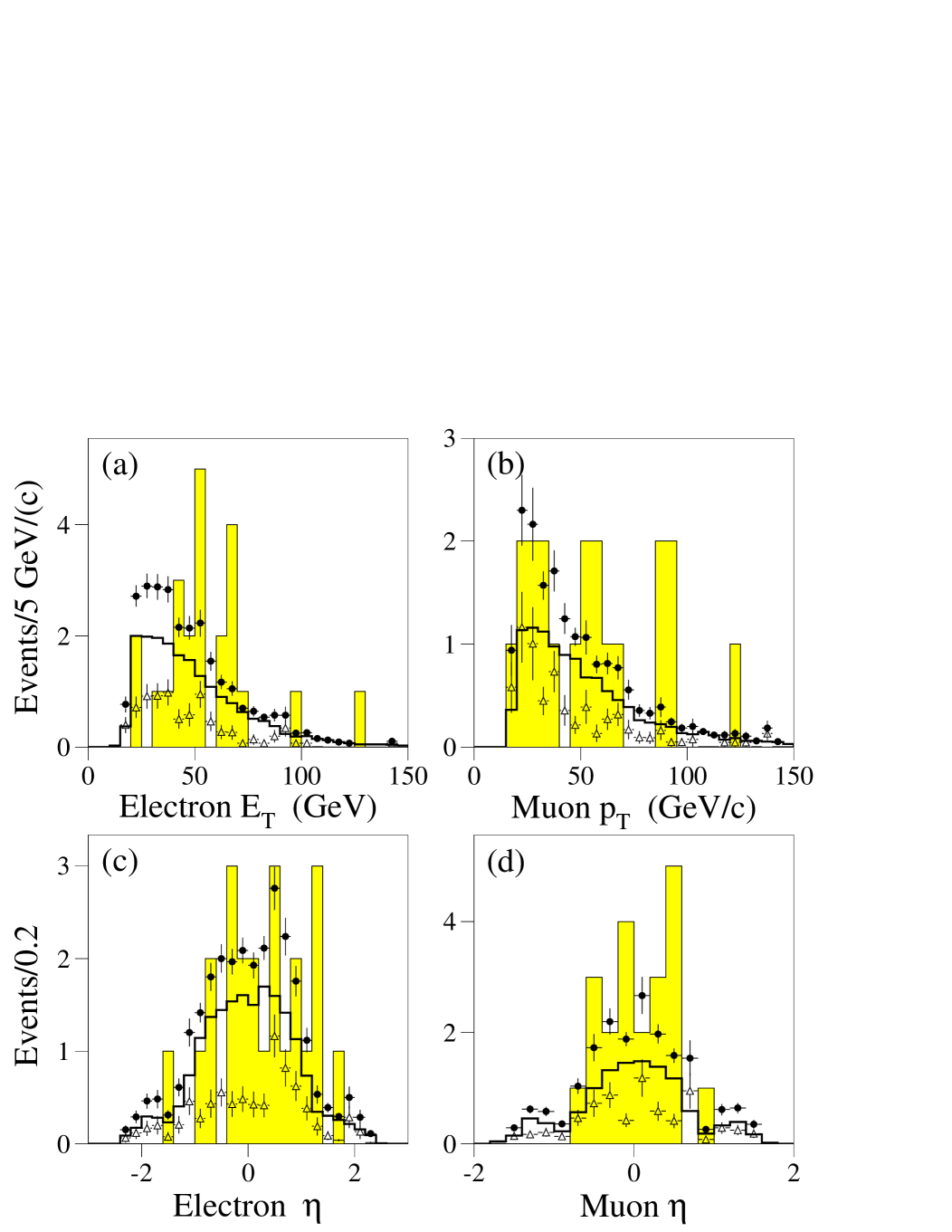
FIG. 31.: $E_{T}$($p_{T}$) and $\eta$ distributions for electrons (muons) for leptonic $t\bar{t}$ candidates (shaded histogram), $t\bar{t}$ MC [herwig, $m_{t}$ = 170 $\mbox{GeV}/c^{2}$] (unshaded histogram), expected background (open triangles), and expected signal plus background (solid circles). The measured muon $p_{T}$ for $e\mu$ candidate 58796-7338(417) is 280.0 GeV/c and is therefore off scale in plot (b). As given in Ref. [104], the event label corresponds to run number and event number (in an early event numbering scheme, this event became well know as “event 417” and thus retains this label parenthetically).

      

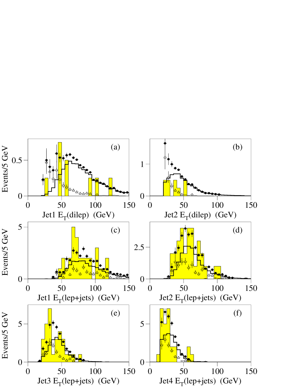
FIG. 32.: Jet $E_{T}$ distributions for dilepton (a)–(b) and $\ell$+jets (c)–(f) $t\bar{t}$ candidates (shaded histogram), $t\bar{t}$ MC [herwig, $m_{t}$ = 170 $\mbox{GeV}/c^{2}$] (unshaded histogram), expected background (open triangles), and expected signal plus background (solid circles). The dilepton candidate histograms [(a)–(b) shaded] have been multiplied by a factor of 0.25 for presentational clarity.

      

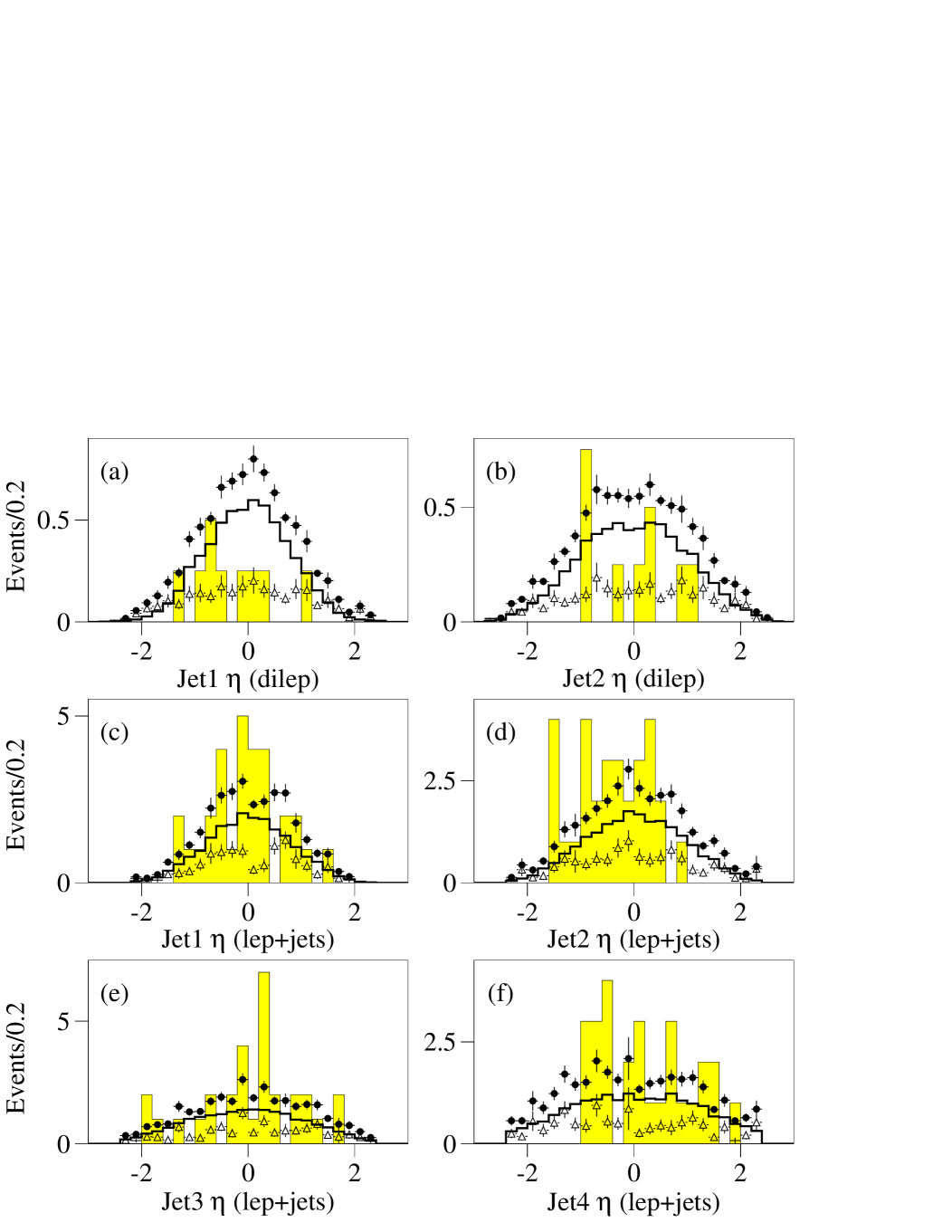
FIG. 33.: Jet $\eta$ distributions for dilepton (a)–(b) and $\ell$+jets (c)–(f) $t\bar{t}$ candidates (shaded histogram), $t\bar{t}$ MC [herwig, $m_{t}$ = 170 $\mbox{GeV}/c^{2}$] (unshaded histogram), expected background (open triangles), and expected signal plus background (solid circles). The dilepton candidate histograms [(a)–(b) shaded] have been multiplied by a factor of 0.25 for presentational clarity.

      

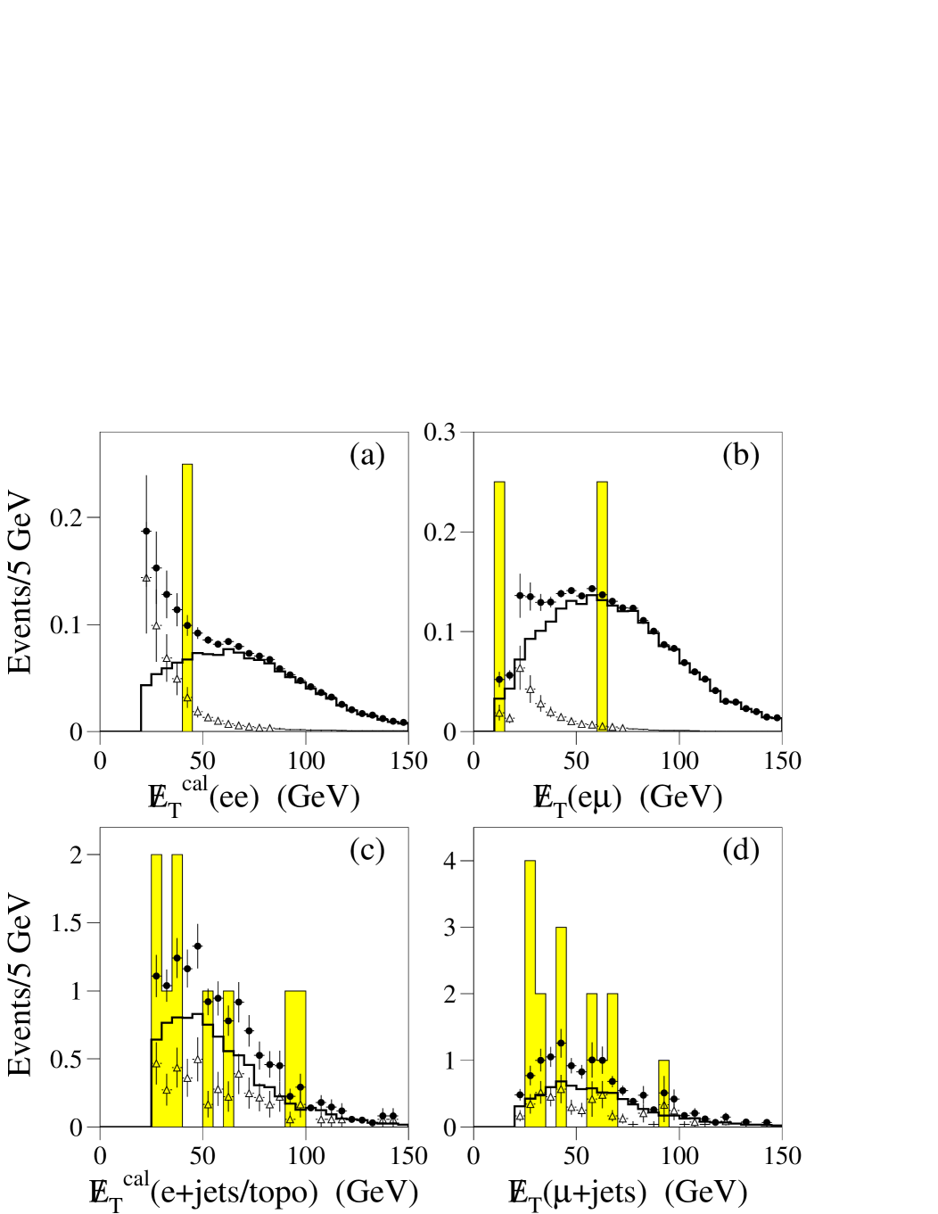
FIG. 34.: ${\hbox{$E$\kern-6.00006pt\lower-0.43057pt\hbox{/}}}_{T}^{\text{cal}}$ distributions for the $ee$ (a) and $e+$jets/topo (c) channels, and $\hbox to0.0pt{\kern 2.5pt/\hss}E_{T}$ distributions for the $e\mu$ (b) and $\mu+$jets/topo and $\mu+$jets/$\mu$ (d) channels: $t\bar{t}$ candidates (shaded histogram), $t\bar{t}$ MC [herwig, $m_{t}$ = 170 $\mbox{GeV}/c^{2}$] (unshaded histogram), expected background (open triangles), and expected signal plus background (solid circles). The $ee$ and $e\mu$ candidate histograms [(a)–(b) shaded] have been multiplied by a factor of 0.25 for presentational clarity. The measured $E\kern-5.70007pt\raise 0.81805pt\hbox{/}_{T}$ for $e\mu$ candidate 58796-7338(417) is 182.9 GeV and is therefore off scale in plot (b).

XI Conclusions

Nine analyses have been described which select event samples dominated by $t\bar{t}$ production. A total of 39 events are found in the leptonic channels with an expected background of $14.0\pm 2.2$. Combining these results with the integrated luminosity and signal efficiency (at $m_{t}$ = 172.1 $\mbox{GeV}/c^{2}$), the $t\bar{t}$ production cross section for the leptonic channels is determined to be

$$5.31\pm 1.34({\rm stat})\pm 1.08({\rm sys})\ {\rm pb}.$$ (59)

This cross section differs slightly from the value reported in Ref. [105] due primarily to an updated luminosity normalization, and to a lesser extent to minor changes in the background estimation for some channels and to the use of a slightly different top mass.

For the all-jets channel, summarized in Sec. VIII and described in detail in Ref. [58], a total of 41 events are found with an expected background of $24.8\pm 2.4$ events. Combining the leptonic and all-jets channels gives a total of 80 candidates with an expected background of $38.8\pm 3.3$ events. This combination results in a $t\bar{t}$ production cross section of

$$5.69\pm 1.21({\rm stat})\pm 1.04({\rm sys})\ {\rm pb}.$$ (60)

As can be seen in Fig. 29, the $t\bar{t}$ production cross sections obtained for the individual channels are in good agreement with the combined cross section and with that from theory [47, 48, 49]. And as shown in Fig. 1(b), the combined cross section is in excellent agreement with DØ’s previously reported values. The current level of uncertainty on QCD predictions for the $t\bar{t}$ production cross section [48, 49] is seen in Fig. 30 to be about $\pm 0.3$ pb, less than 20% of the current experimental uncertainty. Run II of the Fermilab Tevatron is expected to provide an experimental uncertainty on the $t\bar{t}$ cross section of around $\pm 9\%$ ($\approx 0.6$ pb) in 2 ${\rm fb}^{-1}$, limited by systematic uncertainties [106]. This will begin to place restrictions on the various QCD predictions and provide stringent tests for non-standard production and decay mechanisms. In the longer term, the systematic limitations on the measurement of the $t\bar{t}$ production cross section at the CERN Large Hadron Collider is expected to be less than 10% [107].

A Energy Scale Corrections

Gluon radiation and fragmentation can alter a parton’s original energy and direction before its remnants interact and are measured in the calorimeter ($E_{\rm meas}^{\rm jet}$). Also, accompanying spectator interactions, not associated with the hard scattering, can deposit energy within a jet. In addition, fluctuations in interactions in the detector can provide changes to $E_{\rm meas}^{\rm jet}$. For example, emitted particles, especially hadrons, can produce very wide showers in the calorimeter that can affect the fraction of energy ($1-S$) contained within any fixed size cone. Also, most of the absorber is composed of uranium, the radioactive decay of which can deposit significant energy in the calorimeter. Finally, the signal response ($R$) of the calorimeter to a jet is dominated by any difference of response to electrons (or photons) relative to charged hadrons [108, 109], and by any energy deposited in uninstrumented or non-uniform parts of the detector. The energy from spectator interactions and uranium noise provides a total offset ($O$) that must be corrected.

Other than correcting for spectator interactions, only detector effects are considered in the energy calibration of jets. A jet’s particle level energy ($E_{\rm ptcl}^{\rm jet}$) is defined as the energy of a jet found from final state particles using a similar cone algorithm to that used at the calorimeter level. The calibration procedure [109] provides $E_{\rm ptcl}^{\rm jet}$ from $E_{\rm meas}^{\rm jet}$through the relationship:

$$E_{\rm ptcl}^{\rm jet}=\frac{(E_{\rm meas}^{\rm jet}-O)}{R(1-S)}.$$ (A1)

The calibration is performed separately but identically in data and in the Monte Carlo, with the $O$ and $S$ corrections applied to jet energies to extract the particle-level values $E_{\rm ptcl}^{\rm jet}$.

The offset $O$ is estimated as follows. The difference in $E_{T}$ density in ($\eta,\phi$) space between single and double-interaction events, which was obtained with a minimum bias trigger, is defined to be the contribution of the underlying event to single interactions. The contribution from noise is obtained from this same sample by subtracting the $E_{T}$ for the underlying event from the $E_{T}$ density in single interactions. The total systematic uncertainty for the offset in $E_{T}$ density varies from 100  MeV to 300  MeV, depending on the value of $\eta$.

The showering of a jet’s fragments in the calorimeter causes energy to leak out of, or into, any jet cone. To quantify this effect, jets are generated using the herwig program [56], and reconstructed from their original final-state particles. These are subsequently replaced with electron or hadron showers from test beam data, and reconstructed using our cone algorithm, thereby defining a jet shower. The total shower energy is normalized to that of the original final-state particles. The ratio of the contained shower energy to that of the original energy ($\equiv 1-S$) is calculated as a function of $\Delta R$. For central jets with $\Delta R=0.5$, $S$ lies between 0.01 and 0.03, depending on jet energy, with a systematic uncertainty of 1% on $1-S$.

The $\hbox to0.0pt{\kern 2.5pt/\hss}E_{T}$ in direct-photon candidate events (composed of true direct photon events and background dijet events where a $\pi^{0}$ is back to back with a hadronic jet) is used to determine the response of the calorimeter to jets. Differences in response between the photon and the recoiling hadronic system produce an overall imbalance in transverse energy in the calorimeter, giving rise to $\hbox to0.0pt{\kern 2.5pt/\hss}E_{T}$. In these events, the absolute response $R$ of the leading jet can be determined from other well-measured quantities in the event:

$$R=1+\frac{\vec{\mbox{$\hbox to0.0pt{\kern 2.5pt/\hss}E_{T}$}}\cdot{\hat{n}}_{T}^{\gamma}}{\mbox{$E_{T}$}^{\gamma}},$$ (A2)

where $E_{T}^{\gamma}$ ($>15$ GeV) is the transverse energy of the photon and $\hat{n}_{T}$ is the unit vector along the photon’s transverse momentum. Since both the $E_{T}$ of the photon and the direction of the probe jet are well-measured, the energy estimator $E^{\prime}$ can be defined

$$E^{\prime}=E_{T}^{\gamma}{\rm cosh}(\eta_{\rm jet}).$$ (A3)

Measuring the correlation of $R$ with $E^{\prime}$, and $E_{\rm meas}^{\rm jet}$ with $E^{\prime}$, determines the dependence of $R$ on $E_{\rm meas}^{\rm jet}$.

Backgrounds to direct photons are a source of uncertainty for this analysis, particularly in collider data. Instrumental background from highly electromagnetic jets is limited by tight isolation criteria. The residual bias to the measured response is 1.4%. The remaining background consists mostly of $W(\to e\nu)+$jets production, and corresponds to about 0.5%.

In the calibration, because of the rapidly falling photon cross section, energies of central jets are limited to $<150$ GeV. Exploiting the uniformity of the detector, events with EC jets are used to measure the response to higher energy jets. Sensitivity to the number of multiple interactions in an event results in a 2% systematic uncertainty. Because uncertainties in the measurement of the energy scale of low $E_{T}$ jets are quite large, a Monte Carlo direct-photon sample is used for this region, and provides a systematic uncertainty of about 3.5%.

FIG. 35.: Total correction to the energy scale for central ($|\eta|<0.5$) jets.

The total correction is shown in Fig. 35. It rises to a maximum of 1.18 at $E_{T}\simeq 70$ GeV, followed by a slow fall to 1.12 at $E_{T}\simeq 500$ GeV. The upper and lower dashed lines correspond to one standard deviation upper and lower excursions on the total uncertainty, taken as the addition in quadrature of the independent effects discussed above.

B Main-Ring Veto

As noted in Sec. III, particles lost from the Main Ring can affect the measurements of the outer hadronic calorimeter and muon system. The primary losses occur every 2.4 seconds when the protons are injected into the Main Ring and 0.3 seconds later as the beam, which is being accelerated, passes through transition [110]. The injection from the Booster into the Main Ring causes the bunch to widen, and, consequently, a greater amount of beam leaks out of the beampipe. After a few full circuits of the beam in the Main Ring, the bunch coalesces and is mainly confined to the beampipe. Additional losses need to be accounted for in the case when the passage of the proton beam coincides with the $p\bar{p}$ crossing in the Tevatron (which occurs every 3.5 $\mu$s). With each pass, errant particles from the bunch scatter outside the beampipe causing energy deposition in the outer layers of the calorimeter and multiple tracks in the muon system. Because the electromagnetic calorimeter and tracking systems are shielded from these losses, the electron triggers are not significantly impacted. However, jet and especially muon triggers are affected, and it is necessary to veto events from jet, ${\hbox{$E$\kern-6.00006pt\lower-0.43057pt\hbox{/}}}_{T}^{\text{cal}}$, and muon triggers that occur during periods of Main-Ring activity. During the course of the run, several schemes were used to eliminate such events without introducing unnecessary deadtime:

• mrbs-loss (mrbs): The trigger is disabled for 0.4 s after a proton bunch is injected into the Main Ring. This vetoes events during injection and transition and provides a brief recovery time for the muon and calorimeter systems. The typical deadtime for mrbs-loss veto is $\approx 17$%.

• micro-blank (mb): The trigger is disabled for events where Main-Ring bunches are present during the livetime of the muon system which is $\approx\pm 800$ ns centered on the $p\bar{p}$ crossing time. The calorimeter livetime is somewhat longer ($\approx 2\mu$s), so this is therefore not completely efficient for vetoing events with Main-Ring energy in the calorimeter. The typical deadtime for micro-blank is $\approx 7$ %.

• max-live (ml): The trigger is disabled during periods of overlap between mrbs and mb. This corresponds to the first few passes of newly injected beam through the detector.

• good-cal (gc): The trigger is disabled during periods of overlap between mrbs and mb and during mb periods of highest intensity beam leakage. This leakage is measured by a set of scintillator arrays surrounding the Main-Ring beampipe upstream of the DØ detector.

• good-beam (gb): The trigger is disabled during periods of either mrbs or mb. good-beam is the cleanest possible running condition.

The Main-Ring veto used for each trigger is given in Tables 1–5. However, by default, all channels required good-beam for the offline analyses. As will be noted in Secs. C, VI A, and VII A, for the $ee$ and $e$+jets/topo channels it is possible to remove this offline requirement on good-beam and recover a significant fraction of the data lost to it.

C Main-Ring Recovery

As noted in Sec. III, all triggers used in the present analyses, being combinations of electron, muon, jet, and ${\hbox{$E$\kern-6.00006pt\lower-0.43057pt\hbox{/}}}_{T}^{\text{cal}}$ triggers, suffer some loss from the vetoing of events that coincide with activity in the Main Ring. Due to the location of the Main-Ring beam pipe within the detector, the fine hadronic (FH) and electromagnetic sections of the calorimeter and the tracking systems are well shielded from this background, so electron and photon measurements are not significantly affected. However, hadronic jet (and thus ${\hbox{$E$\kern-6.00006pt\lower-0.43057pt\hbox{/}}}_{T}^{\text{cal}}$) and muon measurements are affected. The effect on the hadronic calorimeter gives rise to fake jet backgrounds and mismeasured ${\hbox{$E$\kern-6.00006pt\lower-0.43057pt\hbox{/}}}_{T}^{\text{cal}}$ arising from either large positive signals, if the Main-Ring losses coincide with the Tevatron beam crossing (micro-blank), or from large negative signals for Tevatron beam crossings that were preceded by Main-Ring losses (mrbs). In the latter case, the output voltage of the calorimeter preamps slowly decreases toward zero, causing the difference between a peak and the baseline to become negative. As discussed in the following paragraphs, these effects on the hadronic calorimetry can be minimized with the proper corrections. The effect on the muon system is to decrease the overall muon-finding efficiency by less than 10% during periods of Main-Ring activity, with most of the inefficiency localized to the regions near the Main Ring.

FIG. 36.: Effect of Main-Ring ${\hbox{$E$\kern-6.00006pt\lower-0.43057pt\hbox{/}}}_{T}^{\text{cal}}$ corrections: ${\hbox{$E$\kern-6.00006pt\lower-0.43057pt\hbox{/}}}_{T}^{\text{cal}}$ vs $\phi$ for mrbs events for (a) no correction, (b) CH correction, and (c) total correction.

The $ee$, $e$+jets/topo, and $\mu$+jets/topo channels all retrieve Main-Ring events and correct jets and ${\hbox{$E$\kern-6.00006pt\lower-0.43057pt\hbox{/}}}_{T}^{\text{cal}}$ in the same way.

Normal jets (those from periods when the Main Ring is not active [good-beam]) typically have at most 10% of their energy in the outer, coarse hadronic (CH) region of the calorimeter. During periods of Main-Ring activity (micro-blank), a significant enhancement is seen in the number of jets with $\phi$ values close to that of the Main Ring ($\phi\approx 1.7$), and the vast majority of these jets have CH energy fractions between 60 and 90%. Therefore, for jets in the vicinity of the Main Ring ($1.5<\phi<2.0$) that have CH energy fractions greater than 20%, the CH energy is simply removed [70]. This correction causes the jet $E_{T}$ to be biased low due to the fact that some “real” CH energy is also removed, but as this only affects a small fraction ($<2\%$) of jets in Main-Ring events, it is not a significant concern. Since jets in top quark events are very energetic, the removal of the CH energy typically leaves the jet $E_{T}$ well above threshold. Therefore, the loss in efficiency is minimal, affecting only a small fraction of the 2% of jets in Main-Ring events that are corrected. For events with large negative signals (mrbs) there is also only a small reduction in efficiency, so jets in these events are not corrected.

For ${\hbox{$E$\kern-6.00006pt\lower-0.43057pt\hbox{/}}}_{T}^{\text{cal}}$ the situation is more complicated and requires corrections for both the large positive signals in micro-blank events and the large negative signals in mrbs-loss events. The vast majority of these events are corrected simply by removing the CH energy from the ${\hbox{$E$\kern-6.00006pt\lower-0.43057pt\hbox{/}}}_{T}^{\text{cal}}$ calculation. This can be seen in Fig. 36 which shows ${\hbox{$E$\kern-6.00006pt\lower-0.43057pt\hbox{/}}}_{T}^{\text{cal}}$ vs $\phi$ for mrbs events. Fig. 36(a) is without any correction and shows a large number of events with large ${\hbox{$E$\kern-6.00006pt\lower-0.43057pt\hbox{/}}}_{T}^{\text{cal}}$ pointing towards the Main Ring. As shown in Fig. 36(b), where the CH energy has been removed, most of the events with large ${\hbox{$E$\kern-6.00006pt\lower-0.43057pt\hbox{/}}}_{T}^{\text{cal}}$ pointing towards the Main Ring have been corrected. Although this procedure does remove some positive energy that would normally be included, it does not degrade the ${\hbox{$E$\kern-6.00006pt\lower-0.43057pt\hbox{/}}}_{T}^{\text{cal}}$ resolution appreciably due to the fact that normal (non-Main-Ring) events characteristically have a low ($<10\%$) CH energy fraction. Unfortunately, some events with large ${\hbox{$E$\kern-6.00006pt\lower-0.43057pt\hbox{/}}}_{T}^{\text{cal}}$ in the vicinity of the Main Ring persist after the removal of the CH energy. These events appear primarily in the region of the intercryostat detector (ICD) and massless gap (MG). To correct such events, a vector sum is calculated for all cells in the ICD and MG that have negative energy below a given threshold, and this vector is then subtracted from the ${\hbox{$E$\kern-6.00006pt\lower-0.43057pt\hbox{/}}}_{T}^{\text{cal}}$ vector. These thresholds were determined from comparisons of the negative energy spectra of the ICD and MG cells for good-beam (non-Main-Ring) and mrbs-loss events [70]. In addition to removing all unwanted negative energy, as seen in Fig. 36(c), this procedure brings the ${\hbox{$E$\kern-6.00006pt\lower-0.43057pt\hbox{/}}}_{T}^{\text{cal}}$ resolution to an approximately normal level.

D $e\mu$ Neural Network Analysis

TABLE 34.: Number of observed and expected events passing at each cut level of the $e\mu$ neural network analysis. Expected number of $t\bar{t}$ events are for $m_{t}=170\mbox{$\mbox{GeV}/c^{2}$~{}}$. Uncertainties correspond to statistical and systematic contributions added in quadrature.

Number of events passing $e\mu$ NN selection
		Total	Mis-id	Physics
	Data	sig + bkg	bkg	bkg	$t\bar{t}$
$E_{T}^{e}>15$ GeV, $p_{T}^{\mu}>15$ GeV
+ $e$ id + $\mu$ id + trig	130	$98\pm 12$	$54\pm 2$	$40\pm 9$	$4.3\pm 0.9$
+ $\Delta R({\mu,{\rm jet}})>0.5$, $\Delta R({e,\mu})>0.25$	58	$54\pm 9$	$12\pm 1$	$39\pm 8$	$3.4\pm 0.7$
+ $\mbox{${\hbox{$E$\kern-6.00006pt\lower-0.43057pt\hbox{/}}}_{T}^{\text{cal}}$}>15$ GeV	44	$42\pm 8$	$5.8\pm 0.5$	$32\pm 7$	$3.3\pm 0.7$
+ 2 jets, $E_{T}^{\rm jet}>15$ GeV	6	$4.4\pm 0.9$	$0.68\pm 0.17$	$0.85\pm 0.21$	$2.8\pm 0.7$
+ $O^{\rm comb}_{NN}\geq 0.88$	4	$2.5\pm 0.7$	$0.04\pm 0.12$	$0.19\pm 0.07$	$2.3\pm 0.5$

To further explore this channel, a more sophisticated, independent analysis is also performed. The basic scheme begins with a loose selection and then uses a neural network (NN) to maximize the significance.

This newer analysis is based on the same data set and trigger requirements described in Sec. VI B, and the initial selection is similar. After passing the trigger requirement, events are required to have at least 1 loose electron with $E_{T}>15$ GeV, $|\eta|\leq 2.5$ and at least 1 loose muon with $p_{T}>15$ GeV/$c$. A cut of $\Delta R(\mu,{\rm jet})>0.5$ is then applied to reduce background from QCD multijet events containing a misidentified electron and a non-isolated muon. To remove QCD multijet events in which a misidentified electron and an isolated muon arise from the same jet, a cut of $\Delta R(e,\mu)>0.25$ is applied. As can be seen in Table 34, at this stage the backgrounds from QCD multijet events containing a misidentified electron and an isolated muon from the semi-leptonic decay of a $b$ or $c$ quark and $W(\rightarrow\mu\nu)+$jets events in which one of the jets is misidentified as an electron is still non-negligible. A cut $\mbox{${\hbox{$E$\kern-6.00006pt\lower-0.43057pt\hbox{/}}}_{T}^{\text{cal}}$}\geq 15$ GeV eliminates the multijet events with low ${\hbox{$E$\kern-6.00006pt\lower-0.43057pt\hbox{/}}}_{T}^{\text{cal}}$and rejects the majority of the $W(\rightarrow\mu\nu)+$jet events (as noted above, for $W(\rightarrow\mu\nu)+$jet events, ${\hbox{$E$\kern-6.00006pt\lower-0.43057pt\hbox{/}}}_{T}^{\text{cal}}$ is a measure of the transverse momentum of the $W$ boson). The background at this stage consists primarily of dijet events with a misidentified electron and an isolated muon from semileptonic $b$ or $c$ quark decay (note that the muon momentum contributes to the measured ${\hbox{$E$\kern-6.00006pt\lower-0.43057pt\hbox{/}}}_{T}^{\text{cal}}$). This background is effectively eliminated by requiring two jets with $E_{T}\geq 15$ GeV. At this stage the background is a mixture of QCD multijet (including $W(\rightarrow\mu\nu)+$jet events), $Z/\gamma^{*}\rightarrow\tau\tau\rightarrow e\mu$, and $WW\rightarrow e\mu$ events. For the remaining stages of event selection, neural network techniques are used.

The optimal discrimination between signal and background can be achieved using three separate networks [111]. Each of these discriminates between the signal and one of the dominant backgrounds:

• Network 1 (NN1): $t\bar{t}$ vs QCD multijet events

• Network 2 (NN2): $t\bar{t}$ vs $WW\rightarrow e\mu$ events

• Network 3 (NN3): $t\bar{t}$ vs $Z\rightarrow\tau\tau\rightarrow e\mu$ events

Training is performed on large samples of data (QCD multijet) and MC ($t\bar{t}$, $WW$, $Z\rightarrow\tau\tau$) events. To reduce bias, these samples are prepared with a minimal selection criteria of $E_{T}^{e}\geq 10$ GeV, $p_{T}^{\mu}\geq 10$ GeV/$c$, and $N_{\rm jets}\geq 1$ with $E_{T}^{\rm jet}\geq 10$ GeV. From these, a small sub-sample of 1000–2000 events is selected at random to provide the training sample. The number of nodes and the input parameters for each network are selected to maximize discrimination between signal and background. The best results are obtained using three identical networks, each with six input nodes, seven hidden nodes, and one output node. The input parameters, which consist of five energy and one topological variable for each of the three networks, are listed below:

• Variables used in NN1 and NN2

  • $E_{T}^{e}$, transverse energy of leading electron

  • $E_{T}^{\rm jet2}$, transverse energy of next to leading jet

  • ${\hbox{$E$\kern-6.00006pt\lower-0.43057pt\hbox{/}}}_{T}^{\text{cal}}$, missing transverse energy as measured by the calorimeter

  • $H_{T}^{\rm jets}$, scalar sum of jet transverse energies

    $$H_{T}^{\rm jets}= \displaystyle{\sum_{\rm all\ jets}E_{T}^{\rm jet}},\ {\rm with\ }|\eta^{\rm jet}|\leq 2.5$$

    $${\rm and\ }E_{T}^{\rm jet}\geq 15{\rm\ GeV}$$

  • $M({e\mu})$, electron-muon invariant mass

  • $\Delta\phi({e\mu})$, azimuthal separation of the leading electron and muon

• Variables used in NN3

  • same as NN1 and NN2 except that $E_{T}^{\rm jet1}$ replaces $E_{T}^{\rm jet2}$ (transverse energy of leading jet)

Each of the three networks is trained for 2000 training cycles. Training is started with a set of random weights and thresholds which are adjusted using back propagation as the training proceeded. During training the target outputs are set to unity for signal and zero for background. For simplicity, the outputs of the three networks, $O_{NN1},O_{NN2},O_{NN3}$, are combined into an overall discriminant,

$$O_{NN}^{\rm comb}={3\over{{1\over{O_{NN1}}}+{1\over{O_{NN2}}}+{1\over{O_{NN3}}}}},$$ (D1)

which gives the probability that a given event is signal. The output from such a combination is equivalent to that from a single network that was trained on each of the three different backgrounds and the signal [111]. Testing on independent samples found that a requirement of $O_{NN}^{\rm comb}\geq 0.88$ maximized the relative significance (which is defined to be the ratio of expected number of signal events to the measured uncertainty on the number of background events).

TABLE 35.: Expected number of signal and background events after all cuts in 112.6 ${\rm pb}^{-1}$ for the $e\mu$ neural network analysis. Uncertainties are statistical and systematic contributions added in quadrature. The systematic uncertainty on the total background includes the correlations among the different background sources.

Expected number of $e\mu$ NN evts in 112.6 ${\rm pb}^{-1}$
$t\bar{t}$ MC $m_{t}$ (GeV/$c^{2}$)
150	$3.51\pm 0.86$
160	$2.84\pm 0.68$
170	$2.30\pm 0.53$
180	$1.81\pm 0.41$
$Z\rightarrow\tau\tau\rightarrow e\mu$	$0.10\pm 0.07$
multijet (mis-id $e$)	$0.04\pm 0.12$
$WW\rightarrow e\mu$	$0.08\pm 0.02$
${\rm DY}\rightarrow\tau\tau\rightarrow e\mu$	$0.01\pm 0.01$
Total background	$0.23\pm 0.14$

After this selection four candidate events remain, three of which are also selected by the conventional analysis.

Backgrounds and acceptances are estimated in much the same way as is done for the conventional analysis. The only real difference is that an additional correction is made for the effect of multiple interactions. This correction is obtained by comparing special MC samples with one and two minimum bias events added with the standard MC samples which have no minimum bias events added. The acceptance variation is parameterized as a linear function of the number of interactions and a correction factor is obtained by applying this function to the distribution of the number of interactions throughout Run 1. A correction factor of 9% was found for $t\bar{t}$ events; since the $Z/\gamma^{*}$ and $WW$ backgrounds are kinematically and topologically similar, they receive the same correction. The QCD multijet background, being derived from data, does not require such a correction. The expected numbers of signal and background events passing the full selection are given in Table 35. Figure 37 shows a comparison of data and the expected signal and background as a function of neural network output after all initial cuts except the requirement of 2 jets with $E_{T}>15$ GeV. A cross section of $9.75\pm 5.18({\rm stat})\pm 1.95({\rm sys})$ pb is obtained for the NN-based analysis which is in agreement with the value of $7.1\pm 4.8$ pb obtained for the conventional analysis. Comparison of acceptances and background expectations between the two analyses finds the NN analysis with an increase in acceptance of 10% (for $m_{t}$ = 172 $\mbox{GeV}/c^{2}$) for the same background. Table 34 shows the number of data events, expected signal ($m_{t}=170$ GeV/$c^{2}$), and expected background surviving at each stage of the selection. As with the conventional analysis, good agreement is seen between what is observed and what is expected.

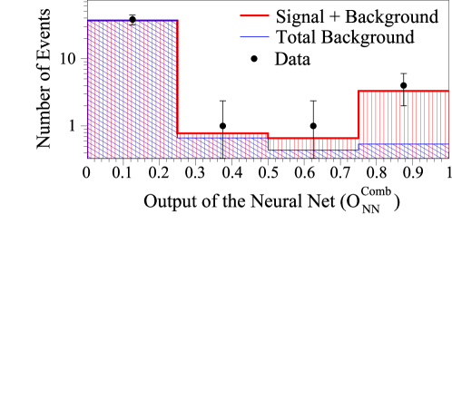
FIG. 37.: Distribution of signal+background (vertical hatching), background (diagonal hatching), and data (circles) as a function of neural network output. All initial cuts have been made except the requirement of 2 jets with $E_{T}>15$ GeV.

TABLE 36.: Efficiency times branching fraction ($\varepsilon\times{\cal B}$) and statistical and systematic uncertainties (in percent), and expected background and corresponding statistical and systematic uncertainties (in number of events), for the $e\mu$ neural network analysis.

		Expected # of Bkg events
	$\varepsilon\times{\cal B}$(%)	$Z\tau\tau$	$WW$	DY$\tau\tau$	Mis-id $e$
	0.351	0.095	0.077	0.006	0.044
Statistical	0.004	0.055	0.006	0.004	0.117
Luminosity	–	0.005	0.004	0.000	–
Energy Scale	0.035	0.026	0.011	0.004	–
$e$ id	0.010	0.004	0.002	0.000	–
High-$p_{T}\ \mu$ id	0.037	0.011	0.008	0.001	–
$e$+jets trig	0.020	0.005	0.004	0.000	–
MC generator	0.025	0.005	0.004	0.000	–
Top quark mass	0.020	–	–	–	–
Bkg crsec	–	0.010	0.008	0.001	–
Other sim	–	0.022	–	–	–
Mis-id $e$	–	–	–	–	0.003
Total	0.065	0.067	0.018	0.005	0.117

Systematic uncertainties are handled the same way as in the conventional analysis and are summarized in Table 36 and, with the exception of the uncertainty on the efficiency times branching fraction due to the top quark mass, are discussed in Sec. IX. The value of $m_{t}$ measured by DØ is $172.1\pm 7.1\mbox{$\mbox{GeV}/c^{2}$~{}}$ [94, 103] and the central value is used in the calculation of the efficiency times branching fraction. This uncertainty of $\pm 7~{}\mbox{$\mbox{GeV}/c^{2}$~{}}$ is composed of an uncertainty of 4.0 $\mbox{GeV}/c^{2}$ due to jet energy scale, 1.9 $\mbox{GeV}/c^{2}$ due to the $t\bar{t}$ MC generator, and 6.1 $\mbox{GeV}/c^{2}$ due to statistics and other sources. The effect of these uncertainties is determined by parameterizing the efficiency times branching fraction as a linear function of top quark mass in the region between 165 and 180 $\mbox{GeV}/c^{2}$. This parameterization is used to convert the above uncertainties on $m_{t}$ into uncertainties on efficiency times branching fraction. The uncertainties on $m_{t}$ due to the jet energy scale and $t\bar{t}$ generator translate into uncertainties on $\varepsilon\times{\cal B}$ of 3.3% and 1.6%, respectively. These uncertainties are combined with the other jet energy scale and $t\bar{t}$ generator uncertainty contributions (described in Sec. IX). The uncertainties on $m_{t}$ due to statistics and from other sources translate into an uncertainty of 5.8% on $\varepsilon\times{\cal B}$, and are included as a separate source of uncertainty in Table 36. As discussed for the conventional dilepton analyses, there is a significant discrepancy between data and MC for the jet $E_{T}$ spectra in $Z+$jet events. The conventional analyses correct for this by taking the jet cut survival probabilities from data and applying them to the MC. Such a procedure is not possible with a NN analysis. Fortunately the primary disagreement between data and MC is in $E_{T}^{\rm jet2}$. It is for this reason that the variables used for NN3 differ from those for NN1 and NN2 in that NN3 employs $E_{T}^{\rm jet1}$ instead of $E_{T}^{\rm jet2}$. To account for the uncertainty due to the initial jet cuts of $N_{\rm jets}\geq 2$ with $E_{T}^{\rm jet}\geq 15$ GeV, a data versus MC comparison was made and a difference of 21% was found. This uncertainty is listed under the category “Other simulation” in Table 36 and is applied only to the $Z\rightarrow\tau\tau$ background.

E Treatment of Uncertainties

As shown in Eq. 58, calculation of the $t\bar{t}$ production cross section requires as input the number of observed events found in all channels, the total expected background, the individual channel acceptance for $t\bar{t}$ events, and the integrated luminosity for each channel. To simplify the discussion, Eq. 58 can be written in the form

$$\sigma(m_{t})_{t\bar{t}}={{\displaystyle N-B}\over{\displaystyle A{\cal L}}}$$ (E1)

where

$$N = \sum_{i}N_{i}$$ (E2)

$$B = \sum_{j}B_{j}$$ (E3)

$$A = {1\over{\cal L}}\sum_{i}A_{i}{\cal L}_{i}$$ (E4)

$${\cal L} = \sum_{i}{\cal L}_{i}.$$ (E5)

with the sum $i$ being over all nine channels and the sum $j$ being over all backgrounds.

It is assumed that the backgrounds and acceptances are subject to the same kinds of uncertainties (see Secs. IX A 1 –  IX A 20) and that no correlation exists among the different uncertainties. With these assumptions, the background error matrix is given by

$$\delta^{2}_{Bij}=\sum_{\mu}\delta^{2}_{B\mu ij},$$ (E6)

where $i$ and $j$ represent the various backgrounds in the different channels (e.g. $W$+jets background in $e$+jets/topo channel), $\mu$ represents the source of uncertainty (e.g. electron identification), and the error matrix for a given uncertainty, $\delta^{2}_{B\mu ij}$, is computed from first principles according to the equation

$$\delta_{B\mu ij}^{2}=\langle B_{i}B_{j}\rangle_{\mu}-\langle B_{i}\rangle_{\mu}\langle B_{j}\rangle_{\mu},$$ (E7)

where the symbol $\langle...\rangle_{\mu}$ represents the average of the enclosed quantity when it is varied according to the uncertainty $\mu$. Accordingly, the correlation matrix for a given uncertainty is given by

$$C_{B\mu ij}={{\delta^{2}_{B\mu ij}}\over{\delta_{B\mu i}\delta_{B\mu j}}},$$ (E8)

where $\delta_{B\mu i}$ is the uncertainty on background $i$ due to source $\mu$.

With these definitions, the uncertainty on the total background is obtained from Eq. E3 by propagation of errors

$$\delta_{B}^{2} = \sum_{ij}\left(\partial B\over\partial B_{i}\right)\left(\partial B\over\partial B_{j}\right)\delta_{Bij}^{2}$$ (E9)

$$= \sum_{ij}\delta_{Bij}^{2}$$ (E10)

$$= \sum_{\mu}\sum_{ij}\delta_{B\mu ij}^{2}$$ (E11)

$$= \sum_{\mu}\left(\delta_{B}\right)_{\mu}^{2},$$ (E12)

where

$$\left(\delta_{B}\right)_{\mu}^{2} = \sum_{ij}\delta_{B\mu ij}^{2}$$ (E13)

$$= \sum_{ij}C_{B\mu ij}\delta_{B\mu i}\delta_{B\mu j}.$$ (E14)

In the case of uncorrelated errors ($C_{B\mu ij}=$ the unit matrix), Eq. E14 reduces to the usual quadratic sum formula,

$$\left(\delta_{B}\right)_{\mu}^{2} = \sum_{i}\delta_{B\mu i}^{2}.$$ (E15)

In the case of maximal positive correlation ($C_{B\mu ij}$ populated entirely by 1’s), Eq. E14 reduces to a linear sum of errors,

$$\left(\delta_{B}\right)_{\mu}^{2} = \left(\sum_{i}\delta_{B\mu i}\right)^{2}.$$ (E16)

For the analyses in this paper, all uncertainties are handled according to one of these two limiting cases. Statistical uncertainties are handled by the quadratic sum formula (Eq. E15) and systematic uncertainties are handled according to the linear sum formula (Eq. E16). The total uncertainty on the background is therefore

$$\delta_{B}^{2}=\sum_{\mu={\rm stat}}\sum_{i}\delta_{B\mu i}^{2}+\sum_{\mu={\rm sys}}\left(\sum_{i}\delta_{B\mu i}\right)^{2}.$$ (E17)

The importance of correlations for the background calculation as a whole depend on the extent to which different backgrounds are affected by the same systematic uncertainties. The systematic uncertainties for all backgrounds to all channels are given in Tables 27 – 29.

Applying the steps above to Eq. E4, the uncertainty on $A$ is found to be

$$\delta_{A}^{2} = {1\over{{\cal L}^{2}}}\sum_{\mu}\sum_{ij}C_{A\mu ij}\delta_{A\mu i}\delta_{A\mu j}{\cal L}_{i}{\cal L}_{j}$$ (E18)

$$= {1\over{{\cal L}^{2}}}\sum_{\mu={\rm stat}}\sum_{i}\delta_{A\mu i}^{2}{\cal L}_{i}^{2}$$ (E20)

$$+{1\over{{\cal L}^{2}}}\sum_{\mu={\rm sys}}\left(\sum_{i}\delta_{A\mu i}{\cal L}_{i}\right)^{2}.$$

Systematic uncertainties on the acceptance ($\varepsilon\times{\cal B}$) are given for all channels in Table 31. Note that the acceptance uncertainties are highly correlated due to the fact that the calculation for each channel is affected by essentially the same set of systematic uncertainties. The same relative uncertainty on the luminosity has been assumed for all channels (see Sec. IX A 1).

The total uncertainty on the top quark cross section is obtained by propagation of errors using Eq. E1. The four inputs to the cross section can, in principle, give rise to six different correlation terms. However, the signal ($N$) has only a statistical uncertainty and the uncertainties on the acceptance ($A$) and the integrated luminosity ($\cal L$) are uncorrelated. Therefore, the only correlation terms are those between the background ($B$) and the acceptance ($A$) and between the background ($B$) and the integrated luminosity ($\cal L$). The corresponding uncertainties are given by the equations

$$\delta_{BA}^{2} = \sum_{\mu}\left(\delta_{BA}\right)_{\mu}^{2}{\rm\ \ \ \ and}$$ (E21)

$$\delta_{B{\cal L}}^{2} = \sum_{\mu}\left(\delta_{B{\cal L}}\right)_{\mu}^{2}.$$ (E22)

The error corresponding to a given uncertainty ($\mu$) is calculated from first principles according to the equations

$$\left(\delta_{BA}\right)_{\mu}^{2} = \langle BA\rangle_{\mu}-\langle B\rangle_{\mu}\langle A\rangle_{\mu}{\rm\ \ \ \ and}$$ (E23)

$$\left(\delta_{B{\cal L}}\right)_{\mu}^{2} = \langle B{\cal L}\rangle_{\mu}-\langle B\rangle_{\mu}\langle{\cal L}\rangle_{\mu},$$ (E24)

where the symbol $\langle...\rangle$ represents the average of the enclosed quantities when they are varied according to the uncertainties $\mu$. The correlation coefficients are given by

$$C_{BA}={{\delta^{2}_{BA}}\over{\delta_{B}\delta_{A}}}{\rm\ \ \ and\ \ \ }C_{B{\cal L}}={{\delta^{2}_{B{\cal L}}}\over{\delta_{B}\delta_{\cal L}}}.$$ (E25)

In the linear/quadratic approximation, these correlation coefficients simplify to

$$C_{BA} = {1\over{\delta_{B}\delta_{A}}}\sum_{\mu}C_{BA\mu}\left(\delta_{B}\right)_{\mu}\left(\delta_{A}\right)_{\mu},$$ (E26)

$$= {1\over{\delta_{B}\delta_{A}}}\sum_{\mu={\rm sys}}\left(\delta_{B}\right)_{\mu}\left(\delta_{A}\right)_{\mu},$$ (E27)

and

$$C_{B{\cal L}} = {1\over{\delta_{B}\delta_{\cal L}}}\sum_{\mu}C_{B{\cal L}\mu}\left(\delta_{B}\right)_{\mu}\left(\delta_{\cal L}\right)_{\mu},$$ (E28)

$$= {1\over{\delta_{B}\delta_{\cal L}}}\sum_{\mu={\rm sys}}\left(\delta_{B}\right)_{\mu}\left(\delta_{\cal L}\right)_{\mu},$$ (E29)

$$= {1\over{\delta_{B}\delta_{\cal L}}}\left(\delta_{B}\right)_{\cal L}\left(\delta_{\cal L}\right),$$ (E30)

$$= {1\over{\delta_{B}}}\left(\delta_{B}\right)_{\cal L}.$$ (E31)

The total uncertainty on the top quark cross section is therefore given by

$$\delta_{{\sigma_{t\bar{t}}}}^{2} = \left(\partial{\sigma_{t\bar{t}}}\over\partial N\right)^{2}\delta_{N}^{2}+\left(\partial{\sigma_{t\bar{t}}}\over\partial B\right)^{2}\delta_{B}^{2}+\left(\partial{\sigma_{t\bar{t}}}\over\partial A\right)^{2}\delta_{A}^{2}$$ (E34)

$$+\left(\partial{\sigma_{t\bar{t}}}\over\partial{\cal L}\right)^{2}\delta_{\cal L}^{2}+\left(\partial{\sigma_{t\bar{t}}}\over\partial B\right)\left(\partial{\sigma_{t\bar{t}}}\over\partial A\right)\delta_{BA}^{2}$$

$$+\left(\partial{\sigma_{t\bar{t}}}\over\partial B\right)\left(\partial{\sigma_{t\bar{t}}}\over\partial{\cal L}\right)\delta_{B\cal L}^{2},$$

$$= {\sigma_{t\bar{t}}}^{2}\left[{\delta_{N}^{2}+\delta_{B}^{2}\over\left(N-B\right)^{2}}+{\delta_{A}^{2}\over A^{2}}+{\delta_{\cal L}^{2}\over{\cal L}^{2}}\right.$$ (E36)

$$\ \ \ \ \ \ \ +{\delta_{B}\over N-B}\left.\left(C_{BA}{\delta_{A}\over A}+C_{B\cal L}{\delta_{\cal L}\over{\cal L}}\right)\right].$$

REFERENCES

- [1] Also at University of Zurich, Zurich, Switzerland.
- [2] Also at Institute of Nuclear Physics, Krakow, Poland.
- [3] CDF Collaboration, F. Abe et al., Phys. Rev. Lett. 74, 2626 (1995).
- [4] DØ Collaboration, S. Abachi et al., Phys. Rev. Lett. 74, 2632 (1995).
- [5] M. L. Perl et al., Phys. Lett. 70B, 487 (1977).
- [6] S. W. Herb et al., Phys. Rev. Lett. 39, 252 (1977).
- [7] M. Kobayashi and T. Maskawa, Prog. Theor. Phys. 49, 652 (1973).
- [8] C. Berger et al., Phys. Lett. 76B, 243 (1978).
- [9] C. W. Darden et al., Phys. Lett. 76B, 246 (1978).
- [10] J. K. Bienlein et al., Phys. Lett. 78B, 360 (1978).
- [11] W. Bartel et al., Phys. Lett. 146B, 437 (1984).
- [12] G. L. Kane and M. E. Peskin, Nucl. Phys. B195, 29 (1982).
- [13] C. Matteuzzi et al., Phys. Lett. 129B, 141 (1983).
- [14] PLUTO Collaboration, C. Berger et al., Phys. Lett. 86B, 413 (1979).
- [15] CELLO Collaboration, H. Behrend et al., Phys. Lett. 144B, 297 (1984).
- [16] AMY Collaboration, H. Sagawa et al., Phys. Rev. Lett. 60, 93 (1988).
- [17] MARKII Collaboration, G. S. Abrams et al., Phys. Rev. Lett. 63, 2447 (1989).
- [18] OPAL Collaboration, M. Akrawy et al., Phys. Lett. B 236, 364 (1990).
- [19] UA1 Collaboration, C. Albajar et al., Z. Phys. C 37, 505 (1988).
- [20] UA1 Collaboration, C. Albajar et al., Z. Phys. C 48, 1 (1990).
- [21] UA2 Collaboration, T. Åkesson et al., Z. Phys. C 46, 179 (1990).
- [22] CDF Collaboration, F. Abe et al., Phys. Rev. Lett. 64, 142 (1990).
- [23] CDF Collaboration, F. Abe et al., Phys. Rev. Lett. 68, 447 (1992).
- [24] DØ Collaboration, S. Abachi et al., Phys. Rev. Lett. 72, 2138 (1994).
- [25] CDF Collaboration, F. Abe et al., Phys. Rev. D 50, 2966 (1994).
- [26] DØ Collaboration, P. Grannis, in Proceedings of the XXVII International Conference on High Energy Physics, Glasgow, Scotland (IOP, Bristol, UK, 1994).
- [27] DØ Collaboration, S. Abachi et al., Phys. Rev. Lett. 79, 1197 (1997).
- [28] CDF Collaboration, F. Abe et al., Phys. Rev. Lett. 80, 2773 (1998).
- [29] CDF Collaboration, T. Affolder et al., Phys. Rev. D 64, 032002 (2001).
- [30] S. Willenbrock and D. Dicus, Phys. Rev. D 34, 155 (1986).
- [31] DØ Collaboration, B. Abbott et al., Phys. Rev. D 63, 031101 (2001).
- [32] DØ Collaboration, V. Abazov et al., Phys. Lett. B 517, 282 (2001).
- [33] J. C. D. Soper and G. Sterman, Nucl. Phys. B263, 37 (1986).
- [34] H. Georgi, S. Glashow, M. Machacek, and D. Nanopoulos, Ann. Phys. 114, 273 (1978).
- [35] L. Jones and H. Wyld, Phys. Rev. D 17, 1782 (1978).
- [36] M. Glück, J. Owens, and E. Reya, Phys. Rev. D 17, 2324 (1978).
- [37] J. Babcock, D. Sivers, and S. Wolfram, Phys. Rev. D 18, 162 (1978).
- [38] K. Hagiwara and T. Yoshino, Phys. Lett. 80B, 282 (1979).
- [39] B. Combridge, Nucl. Phys. B151, 429 (1979).
- [40] P. Nason, S. Dawson, and R. K. Ellis, Nucl. Phys. B303, 607 (1988).
- [41] P. Nason, S. Dawson, and R. K. Ellis, Nucl. Phys. B327, 49 (1989).
- [42] W. Beenakker, H. Kuijf, W. van Neerven, and J. Smith, Phys. Rev. D 40, 54 (1989).
- [43] W. Beenakker et al., Nucl. Phys. B351, 507 (1991).
- [44] M. Mangano, P. Nason, and G. Ridolfi, Nucl. Phys. B373, 295 (1992).
- [45] G. Altarelli, M. Diemoz, G. Martinelli, and P. Nason, Nucl. Phys. B308, 724 (1988).
- [46] R. Ellis, Phys. Lett. B 259, 492 (1991).
- [47] E. Laenen, J. Smith, and W. L. van Neerven, Phys. Lett. B 321, 254 (1994).
- [48] E. Berger and H. Contopanagos, Phys. Rev. D 57, 253 (1998).
- [49] R. Bonciani, S. Catani, M. Mangano, and P. Nason, Nucl. Phys. B529, 424 (1998).
- [50] N. Kidonakis and R. Vogt, Phys. Rev. D 59, 074014 (1999).
- [51] N. Kidonakis, Phys. Rev. D 64, 014009 (2001).
- [52] N. Kidonakis, E. Laenen, S. Moch, and R. Vogt, Phys. Rev. D 64, 114001 (2001).
- [53] DØ Collaboration, B. Abbott et al., Phys. Rev. Lett. 82, 4975 (1999).
- [54] DØ Collaboration, V. M. Abazov et al., Phys. Rev. Lett. 88, 151803 (2002).
- [55] CDF Collaboration, F. Abe et al., Phys. Rev. Lett. 79, 357 (1999).
- [56] G. Marchesini et al., Comp. Phys. Comm. 67, 465 (1992).
- [57] F. A. Berends, H. Kuijf, B. Tausk, and W. T. Giele, Nucl. Phys. B357, 32 (1991).
- [58] DØ Collaboration, B. Abbott et al., Phys. Rev. D 60, 12001 (1999). The all-jets cross section given in this paper is pb.
- [59] H. Baer, V. Barger, and R. J. N. Phillips, Phys. Rev. D 39, 3310 (1989).
- [60] DØ Collaboration, S. Abachi et al., Phys. Rev. D 52, 4877 (1995).
- [61] DØ Collaboration, S. Abachi et al., Nucl. Instrum. Methods Phys. Res. A 338, 185 (1994).
- [62] DØ Collaboration, B. Abbott et al., Phys. Rev. D 61, 072001 (2000).
- [63] CDF Collaboration, F. Abe et al., Phys. Rev. D 50, 5550 (1994).
- [64] E710 Collaboration, N. Amos et al., Phys. Rev. Lett. 68, 2433 (1992).
- [65] E811 Collaboration, C. Avila et al., Phys. Lett. B 445, 419 (1999).
- [66] DØ Collaboration, B. Abbott et al., Phys. Rev. Lett. 80, 3008 (1998).
- [67] DØ Collaboration, B. Abbott et al., Phys. Rev. D 58, 092003 (1998).
- [68] DØ Collaboration, J. Womersley, in Proceedings of the XXVI International Conference on High Energy Physics, Dallas, Texas, edited by J. R. Sanford (AIP, New York, 1993).
-
[69]
E. Varnes, Ph.D. thesis, University of California, Berkeley, 1997
(unpublished), available from http://www-
d0.fnal.gov/results/publications_talks/thesis-
/varnes/thesis.ps. Top quark theses for the DØ
experiment can be found from http://www-d0.fnal.-
gov/results/publications_talks/thesis/Top.html. -
[70]
R. Kehoe, Ph.D. thesis, University of Notre Dame, 1997 (unpublished), available
from http://www-d0.fnal.-
gov/results/publications_talks/thesis/kehoe. -
[71]
P. Tamburello, Ph.D. thesis, University of Maryland, 1997 (unpublished),
available from http://www-d0.-
fnal.gov/results/publications_talks/thesis/tam-
burello/thesis_2sided.ps. - [72] R. Brun et al., geant Detector Description and Simulation Tool, 1993, CERN Program Library Number Q123.
-
[73]
A. J. Milder, Ph.D. thesis, University of Arizona, 1993 (unpublished),
available from http://www-d0.fnal-
.gov/results/publications_talks/thesis/milder/-
diss.ps. - [74] R. V. Astur, Ph.D. thesis, Michigan State University, 1992 (unpublished).
- [75] H. L. Lai et al., Phys. Rev. D 51, 4763 (1995).
- [76] A. Martin, W. Stirling, and R. Roberts, Phys. Lett. B 354, 155 (1995).
- [77] G. Altarelli and G. Parisi, Nucl. Phys. B126, 298 (1977).
- [78] H. Baer, F. E. Paige, S. D. Protopopescu, and X. Tata, BNL Report HET-99/43, Brookhaven (unpublished), http://xxx.lanl.gov/abs/hep-ph/0001086.
- [79] R. Field and R. Feynman, Nucl. Phys. B136, 131 (1978).
- [80] DØ Collaboration, B. Abbott et al., Phys. Lett. B 414, 419 (1997).
- [81] DØ Collaboration, S. Abachi et al., Phys. Lett. B 357, 500 (1995).
- [82] L. Orr, T. Stelzer, and W. Stirling, Phys. Rev. D 52, 124 (1995).
- [83] L. Orr, T. Stelzer, and W. Stirling, Phys. Lett. B 354, 442 (1995).
- [84] T. Sjöstrand, Comp. Phys. Comm. 82, 74 (1994).
- [85] DØ Collaboration, B. Abbott et al., Phys. Rev. D 60, 052003 (1999).
- [86] DØ Collaboration, B. Abbott et al., Phys. Rev. D 61, 032004 (2000).
- [87] R. M. Barnett et al., Phys. Rev. D 54, 1 (1996).
-
[88]
J. McKinley, Ph.D. thesis, Michigan State University, 1996 (unpublished),
available from http://www-d0.-
fnal.gov/results/publications_talks/thesis/mckin-
ley/jtm_thesis.ps. - [89] J. Ohnemus, Phys. Rev. D 50, 1931 (1994).
-
[90]
P. Bloom, Ph.D. thesis, University of California, Davis, 1998 (unpublished),
available from http://www-d0.-
fnal.gov/ pbloom/thesis.html. - [91] DØ Collaboration, N. Amos, in Proc. Intl. Conf. on Computing in High Energy Physics, Rio de Janeiro, Brazil, edited by R. Shellard and T. D. Nguyen (World Scientific, Singapore, 1995).
- [92] V. Barger, J. Ohnemus, and R. J. N. Phillips, Phys. Rev. D 48, 3953 (1993).
- [93] DØ Collaboration, M. Narain, in Proc. Les Recontres de Physique de la Vallée d’Aoste, La Thuile, Italy, edited by M. Greco (World Scientific, Singapore, 1993).
- [94] DØ Collaboration, B. Abbott et al., Phys. Rev. D 58, 052001 (1998).
- [95] S. D. Ellis et al., Phys. Lett. 154B, 435 (1985).
- [96] F. A. Berends et al., Nucl. Phys. B357, 32 (1991).
- [97] E. Berger and H. Contopanagos, Phys. Rev. D54, 3085 (1996).
- [98] DØ Collaboration, S. Abachi et al., Phys. Rev. Lett. 77, 5011 (1996).
- [99] DØ Collaboration, B. Abbott et al., Phys. Rev. Lett. 83, 1908 (1999).
- [100] DØ Collaboration, B. Abbott et al., Nucl. Instrum. Methods Phys. Res. A 424, 352 (1999).
- [101] DØ Collaboration, S. Abachi et al., Phys. Rev. D 53, 6000 (1996).
- [102] DELPHI Collaboration, P. Abreu et al., Z. Phys. C 73, 11 (1996).
- [103] DØ Collaboration, B. Abbott et al., Phys. Rev. D 60, 052001 (1999).
-
[104]
Detailed information on the candidates used in this analysis is available at
http://www-d0.fnal.gov/-
public/top/csec-candidates.ps. - [105] DØ Collaboration, S. Abachi et al., Phys. Rev. Lett. 79, 1203 (1997). The leptonic cross section given in this paper is pb.
- [106] D. Amidei and R. Brock, Future ElectroWeak Physics at the Fermilab Tevatron: Report of the TeV 2000 Study Group, FNAL Report: Pub-96/082.
- [107] F. Gianotti and M. Pepe-Altarelli, Nucl. Phys. B (Proc. Suppl.) 89, 177 (2000), hep-ex/0006016.
- [108] H. Aihara et al., Nucl. Instrum. Methods Phys. Res. A 325, 393 (1993).
- [109] DØ Collaboration, R. Kehoe, in Proceedings of the Sixth International Conference on Calorimetry in High Energy Physics, Frascati, Italy, edited by A. Antonelli, S. Bianco, A. Calcaterra, and F. Fabbri (World Scientific, River Edge, NJ, 1996).
- [110] J. Thompson, FNAL Report TM-1909, Fermilab.
-
[111]
H. Singh, Ph.D. thesis, University of California, Riverside, 1999
(unpublished), available from http://-
www-d0.fnal.gov/results/publications_talks-
/thesis/singh/thesis.ps.