KEK Preprint 2002-11
HUBP-01/02
TU-651
April 2002

Kinematical Reconstruction of the $\bf\it{t\bar{t}}$ System
Near its Threshold at Future $\bf\it{{e^{+}e^{-}}}$ Linear Colliders

Katsumasa Ikematsu^a) , Keisuke Fujii^b) , Zenrō Hioki^c) ,

Yukinari Sumino^d) , Tohru Takahashi^e)

a) Department of Physics, Hiroshima University,

Higashi Hiroshima 739-8526, Japan

b) IPNS, KEK, Tsukuba 305-0801, Japan

c) Institute of Theoretical Physics, University of Tokushima,

Tokushima 770-8502, Japan

d) Department of Physics, Tohoku University,

Sendai 980-8578, Japan

e) Graduate School of Advanced Sciences of Matter, Hiroshima University,

Higashi Hiroshima 739-8530, Japan

ABSTRACT

We developed a new method for full kinematical reconstruction of the $t\bar{t}$ system near its threshold at future linear $e^{+}e^{-}$ colliders. In the core of the method lies likelihood fitting which is designed to improve measurement accuracies of the kinematical variables that specify the final states resulting from $t\bar{t}$ decays. The improvement is demonstrated by applying this method to a Monte-Carlo $t\bar{t}$ sample generated with various experimental effects including beamstrahlung, finite acceptance and resolution of the detector system, etc. A possible application of this method and its expected impact are also discussed.

1 Introduction

The discovery of the top quark [1] at Tevatron has completed the standard-model (SM) list of matter fermions. In spite of its subsequent studies thereat, however, our knowledge on its properties is still far below the level we reached for the lighter matter fermions. A next-generation $e^{+}e^{-}$ linear collider such as JLC [2], having a facet as a top-quark factory, is expected to allow us to measure top quark’s properties with unprecedented precision, thereby improving this situation dramatically. Such precision measurements may shed light on the electroweak-symmetry-breaking mechanism or hint beyond-the-SM physics or both.

Being aware of the opportunities provided by the linear collider, a number of authors have so far taken up this subject and performed interesting analyses [3, 4, 5, 6]. These analyses can be classified into two categories, i.e., those near the $t\bar{t}$ threshold, mainly focused on physics contained in the threshold enhancement factor, and those in open-top region, searching for anomalies in production and decay vertices, both of which play important roles and complement each other. In order to thoroughly carry out such analyses for real data, we need a sophisticated method to kinematically reconstruct events as efficiently and as precisely as possible. This is, however, highly non-trivial in practice, due to finite detector resolutions, possible missing neutrinos in the final states, and various background contributions. We thus need to further explore the potential of the $e^{+}e^{-}$ linear collider and extend the past studies [7, 8, 9] to make maximum use of the linear collider’s advantages: clean experimental environment, well-defined initial state, availability of highly polarized electron beam, possibility of full parton-level reconstruction of final states, etc.

As mentioned above, feasibility studies on form factor measurements are mainly done in the open-top region  [8, 9, 10]. It has, however, been pointed out that form factor measurements in the $t\bar{t}$ threshold region have some favorable features such as availability of well-controlled highly polarized top sample, no need for transformation to $t$ or $\bar{t}$ rest frames because both of the $t$ and $\bar{t}$ are nearly at rest [11, 12]. Besides, as far as the decay form factor measurements of an on-shell top quark are concerned, the center-of-mass energy does not matter. Motivated by these observations, we decided to study feasibility of form factor measurements at the $t\bar{t}$ threshold. From an experimental point of view, the top quark physics at the $e^{+}e^{-}$ linear collider is expected to commence near the $t\bar{t}$ threshold and analysis techniques developed there are expected to be easily extended to the open-top region.

In this paper, we thus aim at state-of-the-art analysis method such as a new method to reconstruct kinematically the $t\bar{t}$ system near its threshold in $e^{+}e^{-}$ annihilation. The content will be divided into six parts. In Sec. 2 we briefly review our simulation framework. Sec. 3 is devoted to top quark reconstruction in the lepton-plus-4-jet mode, where two subsections recapitulate basic strategy and procedure, respectively. In Sec. 4 we explain our kinematical reconstruction method which is designed to improve measurement accuracies of the kinematical variables that specify the final states resulting from $t\bar{t}$ decays. Then we discuss a possible application of this method and its expected impact in Sec. 5. Finally, Sec. 6 summarizes our results and concludes this paper.

2 Framework of Analysis

For Monte-Carlo-simulation studies of $t\bar{t}$ productions and decays, we developed an event generator that is now included in physsim-2001a [17], where the amplitude calculation and phase space integration are performed with HELAS/BASES [18, 19] and parton 4-momenta of an event are generated by SPRING [19]. In the amplitude calculation, initial state radiation (ISR) as well as $S$- and $P$-wave QCD corrections to the $t\bar{t}$ system  [15, 16] are taken into account. Parton showering and hadronization are carried out using JETSET 7.4 [20] with final-state tau leptons treated by TAUOLA [21] in order to handle their polarizations properly.

In this study, the top-quark (pole) mass is assumed to be 175 GeV and the nominal center-of-mass energy is set at 2 GeV-above the $1S$ resonance of the $t\bar{t}$ bound states. This energy is known to be suitable for measurements of various properties of the $t\bar{t}$ system at threshold [7]. We will assume an electron-beam polarization of 80% in what follows. Effects of natural beam-energy spread and beamstrahlung are taken into account according to the prescription given in [7], where the details of the beam parameters are also described. We have assumed no crossing angle between the electron and the positron beams and ignored the transverse component of the initial state radiation. Consequently, the $t\bar{t}$ system in our Monte-Carlo sample has no transverse momentum. Under these conditions we expect 40k $t\bar{t}$ events for 100$fb^{-1}$.

The generated Monte-Carlo $t\bar{t}$ events were passed to a detector simulator (JSF Quick Simulator [22]) which incorporates the ACFA-JLC study parameters (see Table. 1). The quick simulator created vertex-detector hits, smeared charged-track parameters in the central tracker with parameter correlation properly taken into account, and simulated calorimeter signals as from individual segments, thereby allowing realistic simulation of cluster overlapping. It should also be noted that track-cluster matching was performed to achieve the best energy-flow measurements.

Detector	Performance	Coverage
Vertex detector	$\sigma_{\mathrm{b}}=7.0\oplus(20.0/p)\,/\,\sin^{3/2}\theta\;\mu\mathrm{m}$	$|\cos\theta|\leq 0.90$
Central drift chamber	$\sigma_{p_{T}}/p_{T}=1.1\times 10^{-4}p_{T}\>\oplus\>0.1\;\%$	$|\cos\theta|\leq 0.95$
EM calorimeter	$\sigma_{E}/E=15\;\%\>/\sqrt{E}\>\oplus 1\;\%$	$|\cos\theta|\leq 0.90$
Hadron calorimeter	$\sigma_{E}/E=40\;\%\>/\sqrt{E}\>\oplus 2\;\%$	$|\cos\theta|\leq 0.90$

Table 1: ACFA study parameters of the JLC detector, where $p$, $p_{T}$, and $E$ are measured in units of GeV.

3 Event Selection

3.1 Basic Reconstruction Strategy

Since the top quark decays almost 100% into a $b$ quark and a $W$ boson, the signature of a $t\bar{t}$ production is two $b$ jets and two $W$ bosons in the final state. These $W$ bosons decay subsequently either leptonically into a lepton plus a neutrino or hadronically into two jets. According to how the $W$ bosons decay, therefore, there will be three modes of final states: (1) six jets, where both of the $W$’s decay hadronically, (2) one lepton plus four jets, where one of the $W$’s decays leptonically and the other hadronically, and (3) two leptons plus two jets, where both of the $W$’s decay leptonically.

In order to reconstruct the momentum vector of the top quark, we will use the lepton-plus-4-jet mode, for which we can reconstruct the $t$($\bar{t}$)-quark momentum as the momentum sum of the $b$($\bar{b}$) jet and the two jets from the hadronically-decayed $W^{+}$($W^{-}$), while we can tell the charge of the hadronically-decayed $W$ from the charge of the lepton.

In the lepton-plus-4-jet mode, two of the four jets are $b$($\bar{b}$) jets directly from the $t$($\bar{t}$) quarks, while the other two are from the $W$ boson that decayed hadronically. Therefore, if one can identify the $b$ and $\bar{b}$ jets, remaining two jets can be uniquely assigned as decay products of the $W$ boson. The other $W$ boson can be reconstructed from the lepton and the neutrino indirectly detected as a missing momentum. Remaining task is then to decide which $b$($\bar{b}$) jet to attach to which $W$-boson candidate, in order to form $t$($\bar{t}$) quarks. Since the $t$($\bar{t}$) quarks are virtually at rest near the threshold, a $b$($\bar{b}$) jet and the corresponding $W$ boson fly in the opposite directions. We can thus choose the correct combination by requiring the $b$($\bar{b}$) jet and the $W$ boson be approximately back-to-back.

In reality, however, $b$($\bar{b}$)-quark tagging is not perfect and can be performed only with some finite efficiency and purity: there could be more than two $b$($\bar{b}$)-jet candidates in a single event. In addition, $b$ and $\bar{b}$ quarks can be emitted in the same direction. In such a case, a wrong combination could accidentally satisfy the back-to-back condition. These facts sometimes prevent us from uniquely assigning each jet to its corresponding parton, resulting in multiple solutions for a single event. Moreover, the leptonically-decayed $W$ is poorly reconstructed in practice, since the neutrino momentum is strongly affected by ISR, beamstrahlung, as well as other possible neutrinos emitted from the $b$($\bar{b}$) jets. In order to overcome these difficulties, we will need some sophisticated method. We defer discussion of such a method to the next section and examine here the extent to which the aforementioned basic reconstruction strategy works.

3.2 Event Selection Procedure

The lepton-plus-4-jet-mode selection started with demanding an energetic isolated lepton: $E_{\ell}>18~{}{\rm GeV}$ and $E_{14^{\circ}{\rm cone}}<18~{}{\rm GeV}$, where $E_{\ell}$ is the lepton’s energy and $E_{14^{\circ}{\rm cone}}$ is the energy sum of particles within a cone with a half angle of $14^{\circ}$ around the lepton direction excluding the lepton itself. When such a lepton was found, the rest of the final-state particles was forced clustering to four jets, using the Durham clustering algorithm [23]. Two-jet invariant mass was then calculated for each of the six possible combinations and checked if it was between 65 GeV and 95 GeV, in order to select a jet pair which was consistent with that coming from a $W$-boson decay. For such a jet pair the remaining two jets, at the same time, had to be identified as $b$($\bar{b}$) jets, using flavor tagging based on the impact parameter method. The hatched histogram in Fig. 1 is the 2-jet invariant mass distribution of all the possible pairs out of the four jets, while the solid histogram being that with the $b$-tagging. It is seen that this procedure dramatically improved the purity of the $W$ boson sample. It should also be stressed that these selection criteria are very effective to suppress background processes such as $e^{+}e^{-}\rightarrow W^{+}W^{-}$ and provide us with an essentially background-free $t\bar{t}$ event sample.

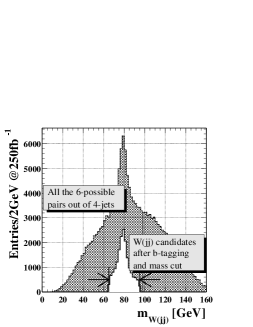
Figure 1: Invariant mass distributions of the 2-jet systems reconstructed as $W$-boson candidates. Hatched and solid histograms correspond to before and after double $b$-tagging, respectively. The locations of the $W$ mass cuts are indicated with arrows.

The remaining task is to decide which $b$($\bar{b}$) jet to associate with which $W$ candidate. For a $b$($\bar{b}$)-jet candidate, the right $W$ boson partner was selected by requiring the back-to-back condition as described above. Fig. 2 is a scatter plot of the acoplanarity angles of the two possible $b$-$W$ systems where horizontal and vertical axes are the angles of $b$-$W_{\ell\nu}$ and $b$-$W_{2-jet}$ system, respectively. $b$-$W$ pairs having $\theta_{acop(b-W)}\leq 60^{\circ}$ was regarded as daughters of the $t$($\bar{t}$) quarks.

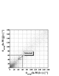
Figure 2: Scatter plot of the acoplanarity angles corresponding to two $b$-$W$ systems, where horizontal and vertical axes are angles of $b$-$W_{\ell\nu}$ and $b$-$W_{2-jet}$ systems, respectively.

The selection efficiency after all of these cuts was found to be 15% including the branching fraction to the lepton-plus-4-jet mode of 29%.

4 Kinematical Fit

The event selection described above yields a very clean $t\bar{t}$ sample. As noted above, however, the sample is still subject to combinatorial backgrounds, if we are to fully reconstruct the final state by assigning each jet to a corresponding decay daughter of the $t$ or $\bar{t}$ quark. We thus need a well-defined criterion to select the best from possible multiple solutions. It is also desirable to improve the measurement accuracies of those kinematical variables which are suffering from effects of missing neutrinos (such variables include momenta of $b$, $\bar{b}$ or the neutrino from a $W$ itself).

The $t\bar{t}$ system produced via $e^{+}e^{-}$ annihilation is a heavily constrained system: there are many mass constraints in addition to the usual 4-momentum conservation. At $e^{+}e^{-}$ linear colliders, thanks to their well-defined initial state and the clean environment, we can make full use of these constraints and perform a kinematical fit to select the best solution and to improve the measurement accuracies of the kinematical variables of the final-state partons.

4.1 Parameters, Constraints, and Likelihood Function

For the lepton-plus-4-jet final state, there are 10 unknown parameters to be determined by the fit: the energies of four jets, the 4-momentum of the neutrino from the leptonically-decayed $W$ boson, and the energies of the initial-state electron and positron, provided that the jet directions as output from the jet finder are accurate enough, the error in the 4-momentum measurement of the lepton from the leptonically-decayed $W$ can be ignored, and that the transverse momenta of the initial-state electron and positron after beamstrahlung or initial-state radiation or both are either negligible or known from a low angle $e^{+}/e^{-}$ detector system (see Fig. 3).

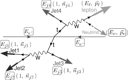
Figure 3: Schematic diagram showing parameters and constraints relevant to the kinematical fit described in the text. The boxed parameters are unknown and to be determined by the fit.

The requirements of 4-momentum conservation and the massless constraint for the neutrino from the leptonically-decayed $W$ reduce the number of free parameters to 5. We choose, as these free parameters, the energies of the four jets and the initial longitudinal momentum (the difference of the energies of the initial-state electron and positron).

These five unknown parameters can be determined by maximizing the following likelihood function:

$$L=(\prod_{f=1}^{4}P^{f}_{E_{f}}(E_{f}^{mean},E_{f}))\cdot P_{\Gamma_{W^{+}}}\cdot P_{\Gamma_{W^{-}}}\cdot P_{\Gamma_{t\bar{t}}}\cdot P_{\sqrt{s}},$$ (1)

where $P^{f}_{E_{f}}$ is a resolution function for jet $f$ and is Gaussian for $f=1$ and $2$ (jets from the hadronically-decayed $W$) as given by the detector energy resolution. For $f=3$ and $4$ (jets from the $b$ and $\bar{b}$ quarks) the resolution function is the same Gaussian convoluted with the missing energy spectrum due to possible neutrino emissions. For the two $W$ bosons in the final state, we use a Breit-Wigner function $P_{\Gamma_{W}}$ instead of $\delta$-function-like mass constraints. $P_{\sqrt{s}}$ is a weight function coming from ISR and beamstrahlung effects. This distribution was calculated as a differential cross section as a function of the energies of initial-state electron and positron, taking into account the $t\bar{t}$ threshold correction as described in Sec. 2.

The remaining factor, $P_{\Gamma_{t\bar{t}}}$, controls the mass distribution of the $t$ and $\bar{t}$ quarks and has been introduced to take into account the kinematical constraint that the $t$ and $\bar{t}$ cannot be simultaneously on-shell below threshold (see Fig. 4 which shows $P_{\Gamma_{t\bar{t}}}$ distribution below $t\bar{t}$ threshold). $P_{\Gamma_{t\bar{t}}}$ distribution is a dynamics-independent factor which is extracted from the theoretical formula for the threshold cross section.

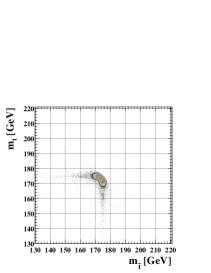
Figure 4: $P_{\Gamma_{t\bar{t}}}$ distribution below $t\bar{t}$ threshold.

4.2 Results

We performed the maximum likelihood fit for the selected sample. The maximum likelihood fit provided us with a well-defined clear-cut criterion to select the best solution, when there were multiple possible solutions for a single event: we should select the one with the highest likelihood.

Figs. 5-a) and -b) are the reconstructed $W$ mass distributions for the leptonically and hadronically-decayed $W$ bosons, respectively, before (hatched) and after (solid) the kinematical fit. The figures demonstrate that the Breit-Wigner factors ($P_{\Gamma_{W^{\pm}}}$) in the likelihood function properly constrain the $W$ masses as intended.

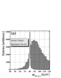
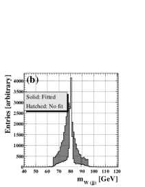
Figure 5: Reconstructed $W$ mass distributions for (a) leptonically and (b) hadronically-decayed $W$ bosons, before (hatched) and after (solid) the kinematical fitting.

Fig. 6-a) plots the reconstructed mass for the $t$($\bar{t}$) decayed into 3 jets against that of the $\bar{t}$($t$) decayed into a lepton plus a $b$ jet, before the kinematical fit. The strong negative correlation is due to the fact that the neutrino from the leptonically-decayed $W$ is reconstructed as the total missing momentum. Figs. 6-b) and -c) are the projections of Fig. 6-a) to the horizontal and vertical axes, respectively, showing systematic shifts of the peak positions. Figs. 6-d) through -f) are similar plots to Figs. 6-a) through -c) after the kinematical fitting, while Figs. 6-g) through -i) are corresponding distributions of generated values (Monte-Carlo truth). The kinematical fit sent most of the events to the L-shaped region indicated in Fig. 6-d), as it should, and made the distribution look like the generated distribution shown in Fig. 6-g). Consequently, the peak shifts observed in the Figs. 6-b) and -c) have been corrected as seen in Figs. 6-e) and -f). There are, however, still some small fraction of events left along the minus $45^{\circ}$ line. These events were so poorly measured that it was impossible to restore. The cut (angled region) indicated in Fig. 6-d) allowed us to remove them without introducing any strong bias on the reconstruction of the kinematical variables.

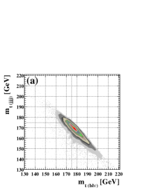
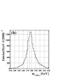
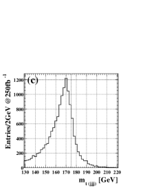
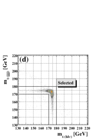
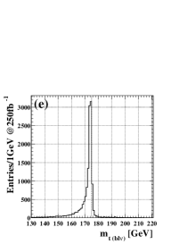
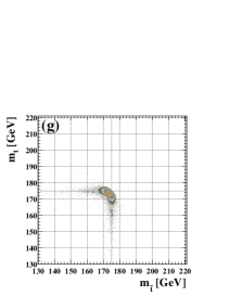
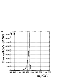
Figure 6: Scatter plot of the reconstructed $t$($\bar{t}$) mass from 3 jets versus that from a lepton plus a $b$-jet (a) before the kinematical fit, together with (b) its horizontal/$b\ell\nu$ and (c) vertical/3-jet projections. (d) through (f) are similar plots after the kinematical fit and (g) though (i) are corresponding plots for generated values.

Now the question is how the above constraints improve the parameters of the fit such as the energies of $b$ and $\bar{b}$ jets, the direction and the magnitude of the missing neutrino from the leptonically-decayed $W$, on which we expect significant influences. Figs. 7-a) and -b) plot the difference between the reconstructed and the generated energies of the $b$ ($\bar{b}$) quark attached to the leptonically-decayed $W$ and that of the $\bar{b}$ ($b$) attached to the hadronically-decayed $W$, respectively, before (hatched) and after (solid) the kinematical fit. The plots demonstrate that the kinematical constraints recover the energies carried away by neutrinos from the $b$ or $\bar{b}$ decays. The improvement is more dramatic for the direct neutrino from the leptonically-decayed $W$, which is reconstructed as the total missing momentum; see Figs. 7-c) and -d) which show distributions of the difference of the reconstructed and generated neutrino energies ($\Delta E_{\nu}$) and directions ($\Delta\theta_{\nu}$).

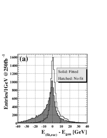
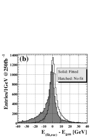
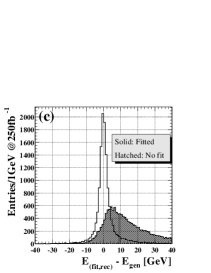
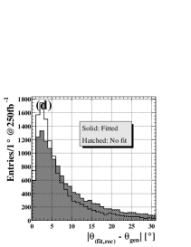
Figure 7: Distributions of the difference of the reconstructed and generated energies of the $b$ or $\bar{b}$ jet attached to (a) leptonically-decayed and (b) hadronically-decayed $W$ bosons, together with distribution of the difference of the reconstructed and generated (c) energies and (d) directions of the direct neutrino from the leptonically-decayed $W$, before (hatched) and after (solid) the kinematical fit.

The improvements in these kinematical variables are reflected to the improvements in the reconstructed $W$ energies and directions as shown in Fig. 8-a) for the energy of the leptonically-decayed $W$, -b) for the hadronically-decayed $W$, and -c) for the direction of the leptonically decayed $W$. We can see dramatic improvements in all of these distributions, although the improvement in the direction of the hadronically-decayed $W$ was less dramatic.

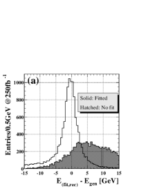
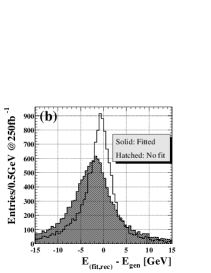
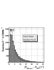
Figure 8: Distributions of the difference of the reconstructed and generated energies of (a) leptonically-decayed and (b) hadronically-decayed $W$ bosons, and (c) distribution of the difference of the reconstructed and generated directions of the leptonically-decayed $W$, before (hatched) and after (solid) the kinematical fit.

Finally, we will examine the effects of the kinematical fit on the measurements of the direction and the magnitude of the top quark momentum. In Figs. 9-a) and -b), the difference of the reconstructed and generated directions of the $t$ or $\bar{t}$ quark is plotted against the generated top momentum, before and after the kinematical fit, respectively. We can see appreciable improvement by the fit. Nevertheless, since the top quark direction becomes more and more difficult to measure as the top quark momentum decreases, the resolution is still somewhat poor in the low momentum region. The angular resolution is largely determined by the reconstruction of the $t$ or $\bar{t}$ decayed into 3 jets. Remember that the resolution improvements were less significant for the hadronically-decayed $W$, since the power of the constraints was used up mostly to recover the momentum information of the direct neutrino from the leptonically-decayed $W$ and the energy resolution for jets from the $W$ was left essentially unimproved. The improvement in the measurements of the top quark direction is mostly coming from the improvement in the $b$ or $\bar{b}$ jet measurement. By the same token, the effect of the fit on the measurement of the magnitude of the top quark momentum is also less dramatic compared to that on the leptonically-decayed $W$.

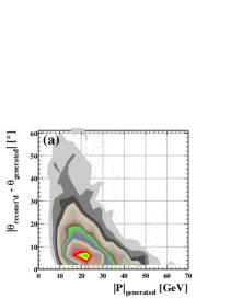
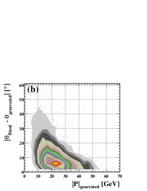
Figure 9: The difference of the reconstructed and generated directions of the $t$ or $\bar{t}$ quark plotted against the generated top momentum, (a) before and (b) after the kinematical fit.

In the case of the 6-jet mode, for which there is no direct energetic neutrino from $W$’s, we can use the power of the constraints to improve the jet energy measurements. Consequently, we may expect more significant improvement in the top quark momentum measurement.

5 A Possible Application

We discuss a possible application of our kinematical reconstruction method. Let us consider measurements of the decay form factors of the top quark in the $t\bar{t}$ threshold region. We assume that deviations of the top-decay form factors from the tree-level SM values are small and consider the deviations only up to the first order, i.e. we neglect the terms quadratic in the anomalous form factors. Then the cross sections depend only on two form factors $f_{1}^{L}$ and $f_{2}^{R}$ in the limit $m_{b}\rightarrow 0$ although the most general $tbW$ coupling includes six independent form factors [26]:

$$\Gamma^{\mu}_{Wtb}=-\frac{g_{W}}{\sqrt{2}}\,V_{tb}\,\bar{u}(p_{b})\biggl{[}\gamma^{\mu}\,f_{1}^{L}P_{L}-\frac{i\sigma^{\mu\nu}p_{W\nu}}{M_{W}}f_{2}^{R}P_{R}\biggr{]}u(p_{t}),$$ (2)

where $P_{L}=(1-\gamma_{5})/2$ and $P_{R}=(1+\gamma_{5})/2$. At tree level of the SM, $f_{1}^{L}=1$ and $f_{2}^{R}=0$. A variation of $f_{1}^{L}$ changes only the normalization of the differential decay width of the top quark, whereas a variation of $f_{2}^{R}$ changes both the normalization and the shape of the decay distributions. Thus, we expect that the kinematical reconstruction is useful for disentanglement of the two form factors and in particular for the measurement of $f_{2}^{R}$. For simplicity we assume $f_{1}^{L}=1$ hereafter. Since transverse $W$ (denoted as $W_{T}$) is more sensitive to $f_{2}^{R}$ than longitudinal $W$ ($W_{L}$), our strategy is to extract $W_{T}$ using the angular distribution of $W$ (in the rest frame of $t$) and the angular distribution of $\ell$ (in the rest frame of $W$). It is well known that $W_{T}$ is enhanced in the backward region $\cos\theta_{W}\simeq-1$, where the angle $\theta_{W}$ is measured from the direction of the top quark spin in the $t$ rest frame. Also, we may enhance $W_{T}$ by collecting $\ell$ emitted in the backward direction $\cos\theta_{\ell}\simeq-1$, where the angle $\theta_{\ell}$ is measured from the direction of $-\vec{p}_{t}$ in the $W$ rest frame. These features are demonstrated in Figs. 10: We plot (a) the differential decay width for the decay of the top quark with a definite spin orientation $d\Gamma(t_{\uparrow}\rightarrow b\ell\nu)/(d\cos\theta_{W}d\cos\theta_{\ell})$ for $f_{2}^{R}=0$ and (b) the difference of the differential widths for $f_{2}^{R}=0.1$ and for $f_{2}^{R}=0$. The plots show that we may measure $f_{2}^{R}$, for instance, from the ratio of the numbers of events in the regions $\cos\theta_{W},\cos\theta_{\ell}<0$ and $\cos\theta_{W},\cos\theta_{\ell}>0$. Since a most prominent result of our kinematical fitting is the improvement in the measurement of the momentum of leptonically decaying $W$, we expect that the sensitivity to $f_{2}^{R}$ would increase after the kinematical fitting.

(a) \psfrag{cosw}{ \hbox{$\cos\theta_{W}$}}\psfrag{cosl}{$\cos\theta_{\ell}$}\includegraphics[height=156.49014pt,clip]{figs/AngularDistSM.eps}           (b) \psfrag{cosw}{ \hbox{$\cos\theta_{W}$}}\psfrag{cosl}{$\cos\theta_{\ell}$}\includegraphics[height=156.49014pt,clip]{figs/AngularDistSMdiff.eps}

Figure 10: (a) Normalized differential decay width ${\cal N}^{-1}\,d\Gamma(t_{\uparrow}\rightarrow b\ell\nu)/(d\cos\theta_{W}d\cos\theta_{\ell})$ for $f_{2}^{R}=0$. (b) Difference of the normalized differential decay widths for $f_{2}^{R}=0.1$ and for $f_{2}^{R}=0$. In both figures the differential widths are normalized by ${\cal N}=\Gamma_{t}\times{\rm Br}(W\rightarrow\ell\nu)$ for $f_{2}^{R}=0$.

It is quite advantageous to investigate decay properties of the top quark in the $t\bar{t}$ threshold region as compared to the open-top region $E\gg 2m_{t}$ because of several reasons. It is useful that the top quark can be polarized close to 100% in the threshold region [27, 28]. This is clear in the above example. Furthermore, we are almost in the rest frame of the top quark. In the above example, the top quark is highly polarized in its rest frame. Hence, the event rate expressed in terms of $\cos\theta_{W}$ and $\cos\theta_{\ell}$ is a direct measure of the amplitude-squared, $|\sum_{i=L,T}{\cal A}(t_{\uparrow}\rightarrow bW_{i})\times{\cal A}(W_{i}\rightarrow\ell\nu)|^{2}$ (without phase-space Jacobian), which allows for simple physical interpretations of event shapes. On the other hand, we do not gain resolving power for the decay form factors by raising the c.m. energy. This is in contrast with the measurements of the $t\bar{t}$ production form factors.

6 Summary and Conclusions

To make maximum use of future $e^{+}e^{-}$ linear colliders’ experimental potential, the top quark reconstruction in the lepton-plus-4-jet mode has been studied under realistic experimental conditions of $e^{+}e^{-}\rightarrow t\bar{t}$ process near its threshold. As a new technique to fully reconstruct $t\bar{t}$ final states, we have developed a kinematical fitting algorithm which aims to reconstruct the momentum-vector of top quark more accurately.

The missing energy carried away by neutrinos from bottom quark decays has been recovered by the kinematical fitting. However, the effects of the kinematical fitting on the top quark momentum are not as dramatic as we wanted. This is because the top quarks are almost at rest in the threshold region and therefore their momenta are difficult to measure. Moreover, in the lepton-plus-4-jet mode many constraints are used up by recovering the information on the neutrino from leptonically-decayed $W$ bosons. On the other hand, the remarkable improvements of the energy resolution of $b$-jets and the angular and energy resolutions of leptonically-decayed $W$’s have been achieved by the kinematical fitting. These improvements should benefit the form factor measurements in general. As a possible application, we considered measurements of decay form factors including $f_{2}^{R}$, on which correct reconstruction of the leptonically-decayed $W$ may have a large impact.

There have been a number of theoretical studies on measurements of the top-quark production and decay form factors using the $e^{+}e^{-}\rightarrow t\bar{t}$ process. Many of these analyses assumed either the most optimistic case or the most conservative case with respect to the kinematical reconstruction of event profiles. In the former case, one assumes that the momenta of all the particles (including $t$ and $W$) can be determined precisely; in the latter case, one uses only partial kinematical information, e.g. the direction of $b$, and the energy and momentum of $\ell$. Our analysis indicates that both assumptions are not the most realistic approximations in actual experimental situations.

As further studies, we will move on to investigate expected sensitivities to various anomalous couplings in the lepton-plus-4-jets mode systematicaly. We also plan to extend the kinematical fitting algorithm to the 6-jet mode, where we expect more significant improvements of the momentum resolution of the top quark and combinatorial background.

Acknowledgements

The authors wish to thank all the members of the ACFA working group for useful discussions and comments. In particular, they are grateful to S. D. Rindani for valuable discussions on strategies for measurements of top quark’s possible anomalous couplings, and A. Miyamoto for improving JSF (JLC Study Framework) to incorporate their requests. This work is partially supported by JSPS-CAS Scientific Cooperation Program under the Core University System and the Grant-in-Aid for Scientific Research No.12740130 and No.13135219 from the Japan Society for the Promotion of Science.

References

-
[1]
CDF Collaboration : F. Abe et al.,
Phys. Rev. Lett. 73, 225 (1994); Phys. Rev. D50, 2966 (1994); Phys. Rev. Lett. 74, 2626 (1995);
D0 Collaboration : S. Abachi et al., Phys. Rev. Lett. 74, 2632 (1995). - [2] JLC group, KEK Report, 92-16 (1992).
- [3] D. Atwood, S. Bar-Shalom, G. Eilam and A. Soni, Phys. Rept. 347, 1 (2001).
- [4] ACFA LC working group, KEK Report, 01-11 (2001), hep-ph/0109166.
- [5] J. A. Aguilar-Saavedra et al. [ECFA/DESY LC Physics Working Group Collaboration], hep-ph/0106315.
- [6] T. Abe et al. [American Linear Collider Working Group Collaboration], in Proc. of the APS/DPF/DPB Summer Study on the Future of Particle Physics (Snowmass 2001) ed. R. Davidson and C. Quigg, SLAC-R-570 Resource book for Snowmass 2001, 30 Jun - 21 Jul 2001, Snowmass, Colorado.
- [7] K. Fujii, T. Matsui and Y. Sumino, Phys. Rev. D50, 4341 (1994).
- [8] T. L. Barklow and C. R. Schmidt, in The Albuquerque Meeting (DPF94) ed. S. Seidel, (World Scientific, 1995).
- [9] R. Frey et al., hep-ph/9704243.
-
[10]
M. Iwasaki [The Linear Collider Detector Group Collaboration],
hep-ex/0102014;
M. Iwasaki, hep-ex/9910065. - [11] S. Gusken, J. H. Kühn and P. M. Zerwas, Phys. Lett. B155, 185 (1985).
- [12] M. Peter and Y. Sumino, Phys. Rev. D57, 6912 (1998).
- [13] G. A. Ladinsky and C. P. Yuan, Phys. Rev. D49, 4415 (1994).
- [14] R. Frey, Proceedings of Workshop on Physics and Experiments with Linear colliders, Morioka-Appi, Japan, Sep. (1995), hep-ph/9606201.
- [15] Y. Sumino, K. Fujii, K. Hagiwara, H. Murayama and C. K. Ng, Phys. Rev. D47, 56 (1993).
- [16] H. Murayama and Y. Sumino, Phys. Rev. D47, 82 (1993).
- [17] physsim-2001a, http://www-jlc.kek.jp/subg/offl/physsim/ .
- [18] H. Murayama, I. Watanabe and K. Hagiwara, KEK Report, 91-11 (1992).
- [19] S. Kawabata, Comp. Phys. Commun. 41, 127 (1986).
- [20] T. Sjöstrand, Comp. Phys. Commun. 82, 74 (1994).
- [21] S. Jadach, Z. Was, R. Decker and J. H. Kühn, Comp. Phys. Commun. 76, 361 (1993).
- [22] JSF Quick Simulator, http://www-jlc.kek.jp/subg/offl/jsf/ .
- [23] S. Catani, Y. L. Dokshitzer, M. Olsson, G. Turnock and B. R. Webber, Phys. Lett. B269, 432 (1991); N. Brown and W. J. Stirling, Z. Phys. C53, 629 (1992).
-
[24]
B. Grzadkowski and Z. Hioki,
Phys. Lett. B529, 82 (2002);
B. Grzadkowski and Z. Hioki, Phys. Lett. B476, 87 (2000). - [25] S. D. Rindani, Pramana 54, 791 (2000).
- [26] G. L. Kane, G. A. Ladinsky and C. P. Yuan, Phys. Rev. D45, 124 (1992).
- [27] R. Harlander, M. Jeżabek, J.H. Kühn and T. Teubner, Phys. Lett. B346, 137 (1995).
- [28] R. Harlander, M. Jeżabek, J. Kühn and M. Peter, Z. Phys. C73, 477 (1997).