Improved $W$ boson mass measurement with the DØ detector

Abstract

We have measured the $W$ boson mass using the DØ detector and a data sample of 82 pb^-1 from the Fermilab Tevatron collider. This measurement uses $W\rightarrow e\nu$ decays, where the electron is close to a boundary of a central electromagnetic calorimeter module. Such ‘edge’ electrons have not been used in any previous DØ analysis, and represent a 14% increase in the $W$ boson sample size. For these electrons, new response and resolution parameters are determined, and revised backgrounds and underlying event energy flow measurements are made. When the current measurement is combined with previous DØ $W$ boson mass measurements, we obtain $M_{W}=80.483\pm 0.084$ GeV. The 8% improvement from the previous DØ measurement is primarily due to the improved determination of the response parameters for non-edge electrons using the sample of $Z$ bosons with non-edge and edge electrons.

I Introduction

In the past decade, many experimental results have improved our understanding of the standard model (SM) sm of electroweak interactions as an excellent representation of nature at the several hundred GeV scale ewwkgp . Dozens of measurements have determined the parameters of the SM, including, indirectly, the mass of the as-yet unseen Higgs boson. The $W$ boson mass measurement plays a critical role in constraining the electroweak higher order corrections and thus gives a powerful constraint on the mechanism for electroweak symmetry breaking.

Recently, direct high precision measurements of $M_{W}$ have been made by the DØ ecmw ; ccmw1b ; ccmw1a and CDF cdfmw collaborations at the Fermilab $\overline{p}p$ collider, and by the ALEPH alephmw , DELPHI delphimw , L3 l3mw and OPAL opalmw collaborations at the CERN LEP-2 $e^{+}e^{-}$ collider. The combined result of these measurements and preliminary LEP-2 updates ewwkgp is $M_{W}=80.451\pm 0.033$ GeV. The combined indirect determination of $M_{W}$ ewwkgp from measurements of $Z$ boson properties at LEP and SLC, taken together with neutrino scattering studies nutevmw and the measured top quark mass topquarkmass , is $M_{W}=80.373\pm 0.023$ GeV, assuming the SM ewwkgp . The reasonable agreement of direct and indirect measurements is an indication of the degree of validity of the SM. Together with other precision electroweak measurements, the $W$ boson measurement favors a Higgs boson with mass below about 200 GeV. Measurement of $M_{W}$ with improved precision is of great importance, as it will enable more stringent tests of the SM, particularly if confronted with direct measurement of the mass of the Higgs boson, or could give an indication of physics beyond the standard paradigm.

The measurements of $M_{W}$ in the DØ experiment use $W$ bosons produced in $\overline{p}p$ collisions at 1.8 TeV at the Fermilab Tevatron collider, with subsequent decay $W\rightarrow e\nu$. The previous measurements are distinguished by the location of the electron in a central electromagnetic calorimeter ($|\eta_{e}|\leq 1.1$) ccmw1b ; ccmw1a or the end calorimeters ($1.5\leq|\eta_{e}|\leq 2.5$) ecmw , where $\eta$ is the pseudorapidity, $\eta=-\ln\tan\theta/2$, and $\theta$ is the polar angle. The measured quantity is the ratio $M_{W}/M_{Z}$, which is converted to the $W$ boson mass using the precision $Z$ boson mass from LEP ewwkgp . Decays of the $Z$ boson into $e^{+}e^{-}$ are crucial for determining many of the detector response parameters. For all previous DØ $W$ boson mass measurements (and for other studies of $W$ and $Z$ boson production and decay), electrons in the central electromagnetic calorimeter were excluded if they were close to the module boundaries in azimuth ($\phi$). In this paper, we revisit the central electron $W$ boson analysis, adding these hitherto unused electron candidates that appear near the calorimeter module boundaries slava . We use a data sample of 82 pb^-1 obtained from the 1994 – 1995 run of the Fermilab collider.

II Experimental method and event selection

II.1 Detector

The DØ detector d0nim for the 1992 – 1995 Fermilab collider run consists of a tracking region that extends to a radius of 75 cm from the beam and contains inner and outer drift chambers with a transition radiation detector between them. Three uranium/liquid-argon calorimeters outside the tracking detectors are housed in separate cryostats: a central calorimeter and two end calorimeters. Each calorimeter has an inner section for detection of electromagnetic (EM) particles; these consist of twenty-one uranium plates of 3 mm thickness for the central calorimeter or twenty 4 mm thick uranium plates for the end calorimeters. The interleaved spaces between absorber plates contain signal readout boards and two 2.3 mm liquid argon gaps. There are four separate EM readout sections along the shower development direction. The transverse segmentation of the EM calorimeters is 0.1$\times$0.1 in $\Delta\eta\times\Delta\phi$, except near the EM shower maximum, where the segmentation is 0.05$\times$0.05 in $\Delta\eta\times\Delta\phi$. Subsequent portions of the calorimeter have thicker uranium or copper/stainless steel absorber plates and are used to measure hadronic showers. The first hadronic layer is also used to capture any energy escaping the EM layers for electrons or photons. The muon detection system outside the calorimeters is not used in this measurement, except as outlined in Refs. ecmw ; ccmw1b ; ccmw1a for obtaining a muon track sample used to calibrate the drift chamber alignment.

An end view of the central calorimeter is shown in Fig. 1. There are three concentric barrels of modules; the innermost consists of thirty-two EM modules, followed by sixteen hadronic modules with 6 mm uranium absorber plates, and then sixteen coarse hadronic modules with 40 mm copper absorber plates to measure the tails of hadronic showers. All previous DØ $W$ boson mass analyses using central electrons have imposed cuts on the electron impact position in the EM modules that define a fiducial region covering the interior 80% in azimuth of each module. Such electrons will be referred to in this paper as ‘C’ or ‘non-edge’ electrons. The remaining central electrons that impact on the two 10% azimuthal regions near an EM module edge suffer some degradation in identification probability and energy response, but are typically easily recognizable as electrons. We will refer to them as ‘$\widetilde{\rm C}$’ or ‘edge’ electrons. The edge region corresponds to about 1.8 cm on either side of the EM module. Those electrons identified in the end calorimeters ecmw are labelled ‘E’. The end calorimeters have a single full azimuth module and consequently have no edges. Dielectron pair samples are denoted CC, $\widetilde{\rm C}$C, $\widetilde{\rm C}$$\widetilde{\rm C}$, CE, $\widetilde{\rm C}$E, or EE according to the location of the two electrons.

Figure 1: End view of the central calorimeter showing the arrangement for electromagnetic (EM), fine hadronic (FH) and coarse hadronic (CH) modules. The Tevatron Main Ring passes through the circular hole near the top of the CH ring.

The detailed constitution of the EM calorimeter in the vicinity of the edges of two modules is shown in Fig. 2. The mechanical support structure for the modules is provided by thick stainless steel end plates (not shown); the end plates of adjacent modules are in contact to form a 32-fold polygonal arch. The elements of each module are contained within a permeable stainless steel skin to allow the flow of liquid argon within the cryostat. Adjacent module skins are separated by about 6 mm. The uranium absorber plates extend to the skins, so that any electron impinging upon the module itself will pass through sufficient material to make a fully developed EM shower. Within the gaps between absorber plates, G10 signal boards are etched on both sides to provide the desired $\eta-\phi$ segmentation for readout. The signal boards are coated on both sides with resistive epoxy and held at a voltage of 2 kV to establish the electric field within which ionization drifts to the signal boards. The resistive coat is set back from the ends of the board by about 3 mm to avoid shorts to the skin. In the region of this setback, the electric field fringing causes low ion drift velocity and thus reduced signal size, but the shower development is essentially normal as the absorber configuration is standard. The hadronic calorimeter modules are rotated in azimuth so that the edges of EM and hadronic modules are not aligned.

Figure 2: Construction of central calorimeter EM modules in the region near module boundaries. Signal boards have the electrode pads for signal collection; readout boards carry traces bringing the signals to the module ends.

The directions of electrons and their impact point on the calorimeter are determined ccmw1b ; ccmw1a using the central drift chamber (CDC), located just inside the calorimeter cryostat. This chamber has four azimuthal rings of thirty-two modules each. In each module, the drift cell is defined with seven axial sense wires and associated field shaping wires. The ring 2 and 4 sense wire azimuthal locations are offset by one half cell from those of rings 1 and 3. Half of the sense wires are aligned in azimuth with a calorimeter edge and the other half are aligned with the center of a calorimeter module. The drift chamber $z$-coordinate parallel to the beam is measured by delay lines in close proximity to the inner and outer sense wires of each module, using the time difference of arrival at the two ends.

II.2 Triggers

Triggers for the $W$ boson mass analysis, described in more detail in Refs. ecmw ; ccmw1b ; ccmw1a , are derived primarily from calorimetric information. For the hardware level 1 trigger, calorimeter signals are ganged into $\Delta\eta\times\Delta\phi=0.2\times 0.2$ towers in both EM and hadronic sections. Energy above a threshold is required for a seed EM tower. The hardware refines this to include the maximum transverse energy tower adjacent to the seed, and requires this combination to exceed a fixed threshold. The corresponding hadronic tower transverse energy must not exceed 15% of the EM tower energy. The second level trigger refines the information in computer processors using a more sophisticated clustering algorithm. At level 2, the missing transverse energy ($\hbox to0.0pt{\kern 1.49994pt/\hss}E_{T}$) components are formed. The $W$ boson level 2 trigger requires an EM cluster and $\hbox to0.0pt{\kern 1.49994pt/\hss}E_{T}$ above a threshold. The $Z$ boson level 2 trigger requires two EM clusters. In addition, trigger requirements are imposed to ensure an inelastic collision, signalled by scintillators near the beam lines, and require the event to be collected outside times where beam losses are expected to occur ecmw . For the offline cuts described below, the triggers are 100% efficient ccmw1b ; slava .

II.3 Data Selection

The offline data selection cuts are the same as in the previous DØ $W$ boson mass analyses. The variables used for event selection are:

• Electron track direction: The track azimuth of a C or $\widetilde{\rm C}$ electron is determined from the CDC track centroid and the reconstructed transverse vertex position (determined from the drift chamber measurement of tracks). We define the axial track center of gravity in the CDC as $z_{\rm trk}$. The track pseudorapidity is then determined from the difference between $z_{\rm trk}$ and the EM calorimeter cluster center of gravity.

• Distance of the electron from calorimeter module edge: The distance along the front face of the EM calorimeter module from the module edge is measured by the extrapolation of the line from the event vertex through the central drift chamber track centroid. The azimuthal distance from the module edge is denoted $d_{\rm edge}$.

• Calorimeter energy location: $\eta_{\rm det}$ is the pseudorapidity of the EM cluster in the calorimeter, measured from the center of the detector. The axial position of the EM cluster in the EM calorimeter is denoted by $z_{\rm clus}$.

• Shower shape: The covariance matrix of energy deposits in forty lateral and longitudinal calorimeter subdivisions and the primary vertex $z$ position are used to define a chisquare-like parameter, $\xi_{\rm shape}$, that measures how closely a given shower resembles test beam and Monte Carlo EM showers hmatrix .

• Electron isolation: the calorimeter energies are used to define an isolation variable, $f_{\rm iso}=(E_{\rm full}-E_{\rm core})/E_{\rm core}$, where $E_{\rm core}$ is the energy in the EM calorimeter within $\mathcal{R}$=0.2 of the electron direction, $E_{\rm full}$ is the energy in the full calorimeter within $\mathcal{R}$=0.4 and $\mathcal{R}=\sqrt{\Delta\eta^{2}+\Delta\phi^{2}}$.

• Track match significance: $\sigma^{2}_{\rm trk}=(\Delta s/\delta s)^{2}+(\Delta\zeta/\delta\zeta)^{2}$ measures the quality of the track match, where $s$ is the $r\phi$ coordinate and $\zeta$ is the $z$ coordinate for the central calorimeter or radial coordinate for the end calorimeter. $\Delta s$ and $\Delta\zeta$ are the differences between track projection and shower maximum coordinates in the EM calorimeter, and $\delta s$ and $\delta\zeta$ are the corresponding errors ecmw ; ccmw1b .

• EM fraction: the fraction, EMF, of energy within a cluster that is deposited in the EM portion of the calorimeter.

• Electron likelihood: a likelihood variable, $\lambda_{4}$, based upon a combination of EMF, $\sigma_{\rm trk}$, $dE/dx$ in the CDC, and $\xi_{\rm shape}$ fourlikelihood .

• Kinematic quantities: the transverse momenta of electrons, neutrinos, and the $W$ or $Z$ bosons are denoted $p_{T}(e),p_{T}(\nu),p_{T}(W)$ or $p_{T}(Z)$. The $p_{T}(\nu)$ is determined from the missing transverse energy in the event, as discussed below. The invariant mass of two electrons is denoted by $m_{ee}$.

The requirements for central and end electrons are given in Table 1.

Table 1: Offline selection criteria for central and end electron candidates.

Variable	Central Electron	End Electron
$|\eta_{\rm det}|$	$\leq 1.1$	$1.5-2.5$
$\xi_{\rm shape}$	$\leq 100$	$\leq 200$
$\sigma_{\rm trk}$	$\leq 5$	$\leq 10$
EMF	$\geq 0.90$	$\geq 0.90$
$f_{\rm iso}$	$\leq 0.15$	$\leq 0.15$
$\lambda_{4}$	–	$\leq 4.0$
$|z_{\rm clus}|$	$\leq 108$ cm	–
$|z_{\rm trk}|$	$\leq 80$ cm	–

The selection criteria for the $W$ and $Z$ boson event samples are given in Table 2. Non-edge electrons are defined as those with $d_{\rm edge}$/$d_{\rm mod}\geq 0.1$, where $d_{\rm mod}$ is the full width of the module in azimuth. Edge electrons are required to have $d_{\rm edge}$/$d_{\rm mod}$ $<0.1$. For the $Z$ boson sample with two electrons in the central calorimeter, both are required to have good tracks in the drift chamber (i.e. passing the $\sigma_{\rm trk}$ requirement) if either of them is in a central calorimeter edge region; if both are non-edge, only one electron is required to have a good track. For $Z$ boson samples with one electron in the end calorimeter, the end electron must have a good track, while the central electron is required to have a good track only if the electron is in the edge region.

Table 2: Event selection criteria for $W$ and $Z$ boson samples.

Variable	$W$ boson sample	$Z$ boson sample
$p_{T}(e{\rm~{}central})$	$\geq 25$ GeV	$\geq 25$ GeV
$p_{T}(e{\rm~{}end})$	–	$\geq 30$ GeV
$p_{T}(\nu)$	$\geq 25$ GeV	–
$p_{T}(W)$	$\leq 15$ GeV	–
$m_{ee}$	–	60 – 120 GeV
$|z_{\rm vtx}|$	$\leq 100$ cm	$\leq 100$ cm

With these selections, we define three $W$ boson samples and six $Z$ boson samples, differentiated by whether the electrons used are C, $\widetilde{\rm C}$, or E. The numbers of events selected in each sample are given in Table 3.

Table 3: Event sample sizes.

$W$ boson sample	No. events	$Z$ boson sample	No. events
C	27,675	CC	2,012
$\widetilde{\rm C}$	3,853	$\widetilde{\rm C}$C	470
E	11,089	$\widetilde{\rm C}$$\widetilde{\rm C}$	47
		CE	1,265
		$\widetilde{\rm C}$E	154
		EE	422

II.4 Experimental method

The experimental method used in this work closely resembles that of previous DØ $W$ boson mass measurements. We compare distributions from the $W$ and $Z$ boson samples with a set of templates of differing mass values, prepared using a fast Monte Carlo program that simulates vector boson production and decay, and incorporates the smearing of experimentally observed quantities using distributions derived from data. The variables used for the $W$ boson templates are the transverse mass,

$$m_{T}=\sqrt{2p_{T}(e)p_{T}(\nu)[1-\cos(\phi_{e}-\phi_{\nu})]},$$ (1)

and the transverse momenta of the electron and neutrino, $p_{T}(e)$ and $p_{T}(\nu)$. The three distributions depend on a common set of detector parameters, but with different functional relationships, so that the measurements from the three distributions are not fully correlated. As discussed in Ref. ecmw , the $m_{T}$ distribution is affected most by the hadronic calorimeter response parameters, whereas the $p_{T}(e)$ distribution is mainly broadened by the intrinsic $p_{T}(W)$ distribution, and the $p_{T}(\nu)$ distribution is smeared by a combination of both effects. The $Z$ boson template variable is the invariant mass, $m_{ee}$.

The observed quantities used for $W$ boson reconstruction are $p_{T}(e)$ and the recoil transverse momentum, $\vec{u}_{T}=\Sigma_{i}E_{Ti}\hat{n}_{i}$, where $\hat{n}_{i}$ is the unit vector pointing to calorimeter cell $i$, and the sum is over all calorimeter cells not included in the electron region. The electron energy in the central calorimeter is summed over a $\Delta\eta\times\Delta\phi$ region of $0.5\times 0.5$ centered on the most energetic calorimeter cell in the cluster. Note that this region spans 2.5 modules in azimuth, so always contains several module edges irrespective of the electron impact point. For the end calorimeter, the electron energy sum is performed within a cone of radius 20 cm (at shower maximum), centered on the electron direction. In both cases energy from the EM calorimeter and first section of the hadron calorimeter is summed.

The neutrino transverse momentum in $W$ boson decays is taken to be $\vec{p}_{T}(\nu)=-\vec{p}_{T}(e)-\vec{u}_{T}$. The components of $\vec{u}_{T}$ in the transverse plane are most conveniently taken as $u_{\parallel}=\vec{u}_{T}\cdot\hat{e}$ and $u_{\perp}=\vec{u}_{T}\cdot(\hat{e}\times\hat{z})$, where $\hat{e}$ ($\hat{z}$) is the electron (proton beam) direction.

The momentum $\vec{p}(ee)=\vec{p}(e_{1})+\vec{p}(e_{2})$ and the dielectron invariant mass define the dielectron system for the $Z$ boson sample. The dielectron transverse momentum is expressed in components along the inner bisector axis $\hat{\eta}$ of the two electrons, and the transverse axis $\hat{\xi}$ perpendicular to $\hat{\eta}$.

The data are compared with each of the templates in turn and a likelihood parameter $\mathcal{L}$ is calculated. The set of likelihood values at differing boson masses and fixed width is fitted to find the maximum value, corresponding to the best measurement of the mass. Statistical errors are determined from the masses at which $\ln\mathcal{L}$ decreases by one-half unit from this maximum.

II.5 Monte Carlo production and decay model

The production and decay model is taken to be the same as for the earlier measurements ecmw ; ccmw1b ; ccmw1a . The Monte Carlo production cross section is based upon a perturbative calculation ladinskyyuan which depends on the mass, pseudorapidity, and transverse momentum of the produced boson, and is convoluted with the MRST parton distribution functions mrst . We use the mass-dependent Breit-Wigner function ccmw1b with measured total width parameters $\Gamma_{W}$ and $\Gamma_{Z}$ to represent the line shape of the vector bosons. The line shape is modified by the relative parton luminosity as a function of boson mass, due to the effects of the parton distribution function. The parameter $\beta$ in the parton luminosity function $\mathcal{L}_{q\overline{q}}=e^{-\beta m_{ee}}/m_{ee}$ is taken from our previous studies ecmw ; ccmw1b .

Vector boson decays are simulated using matrix elements which incorporate the appropriate helicity states of the quarks in the colliding protons and antiprotons. Radiative decays of the $W$ boson are included in the Monte Carlo model ccmw1b based on the calculation of Ref. behrends . Decays of the $W$ boson into $\tau\nu$ with subsequent $\tau\rightarrow e\nu\overline{\nu}$ decays are included in the Monte Carlo, properly accounting for the $\tau$ polarization ccmw1b .

II.6 Monte Carlo detector model

The Monte Carlo detector model employs a set of parameters for responses and resolutions taken from the data ccmw1b . Here we summarize these parameters and indicate which are re-evaluated for the edge electron analysis.

The observed electron energy response is taken to be of the form

$$E^{\rm meas}=\alpha E^{\rm true}+\delta.$$ (2)

The scale factor $\alpha$ that corrects the response relative to test beam measurements is determined using fits to the $Z$ boson sample; for the C electrons, $\alpha=0.9540\pm 0.0008$. The energy offset parameter $\delta$ correcting for effects of uninstrumented material before the calorimeter is found from fits to the energy asymmetry of the two electrons from $Z$ bosons, and from fits to $J/\psi\rightarrow e^{+}e^{-}$ and $\pi^{0}\rightarrow\gamma\gamma\rightarrow(e^{+}e^{-})(e^{+}e^{-})$ decays. For C electrons, $\delta=-0.16^{+0.03}_{-0.21}$. There is an additional energy correction (not shown in Eq. 2) that contains the effects of the luminosity-dependent energy depositions within the electron window from underlying events, and also corrects for the effects of noise and zero suppression in the readout. This correction is made using observed energy depositions in $\eta-\phi$ control regions away from electron candidates. We discuss the modification of the energy response parametrization for $\widetilde{\rm C}$ electrons below.

The electron energy resolution is taken as

$${\sigma_{E}\over E}={s\over\sqrt{E}}\oplus c\oplus{n\over E},$$ (3)

where $\oplus$ indicates addition in quadrature. The sampling term constant $s$ is fixed at the value obtained from test beam measurements, and the noise term $n$ is fixed at the value obtained from the observed uranium and electronics noise distributions in the calorimeter. The constant term $c$ is fitted from the observed $Z$ boson line shape. The parameter values for C electrons ccmw1b are $s=0.135$ (GeV^1/2), $c=0.0115^{+0.0027}_{-0.0036}$, and $n=0.43$ GeV. The resolution parameters are re-evaluated for $\widetilde{\rm C}$ electrons below.

The transverse energy is obtained from the observed energy using $E_{T}=E\sin\theta$, where the polar angle is obtained as indicated in Sec. IIC, with the errors taken from the measurements of electron tracks in $Z$ boson decays.

The efficiency for electron identification depends on the amount of recoil energy, $u_{\parallel}$, along the electron direction. We take this efficiency to be constant for $u_{\parallel}<u_{0}$ and linearly decreasing with slope $s_{0}$ for $u_{\parallel}>u_{0}$. The parameters of this model for the efficiency are determined by superimposing Monte Carlo electrons onto events from the $W$ boson signal sample with the electron removed, and then subjecting the event to our standard selection cuts. For non-edge electrons, $u_{0}=3.85$ GeV and $s_{0}=-0.013$ GeV^-1; these parameters are strongly correlated ccmw1b . Since the properties of electrons in the edge region are different from those in the non-edge region, we re-examine this efficiency below for the $\widetilde{\rm C}$ sample.

The unsmeared recoil transverse energy is taken to be

$$\vec{u}_{T}=-(R_{\rm rec}~{}\vec{q}_{T})-\Delta u_{\parallel}~{}\hat{p}_{T}(e)+\alpha_{\rm mb}~{}\hat{m},$$ (4)

where $\vec{q}_{T}$ is the generated $W$ boson transverse momentum; $R_{\rm rec}$ is the response of the calorimeter to recoil (mostly hadronic) energy; $\Delta u_{\parallel}$ is a luminosity- and $u_{\parallel}$-dependent correction for energy flow into the electron reconstruction window; $\alpha_{\rm mb}$ is a correction factor that adjusts the resolution to fit the data, and is roughly the number of additional minimum bias events overlaid on a $W$ boson event; and $\hat{m}$ is the unit vector in the direction of the randomly distributed minimum bias event transverse energy. The response parameter is parametrized as $R_{\rm rec}=\alpha_{\rm rec}+\beta_{\rm rec}\log q_{T}$ and is measured using the momentum balance in the $\hat{\eta}$ (dielectron bisector) direction for the $Z$ boson and the recoil system. The $\Delta u_{\parallel}$ parameter due to recoil energy in the electron window is similar to the corresponding correction to the electron energy, but is modified to account for readout zero-suppression effects. The recoil response is due to energy deposited over all the calorimeter, and thus is not expected to be modified for the $\widetilde{\rm C}$ electron analysis.

The recoil transverse energy resolution is parameterized as a Gaussian response with $\sigma_{\rm rec}=s_{\rm rec}\sqrt{u_{T}}$, modified by the inclusion of a correction for luminosity-dependent event pileup controlled by the $\alpha_{\rm mb}$ parameter introduced above. These parameters are fit from the $Z$ boson events using the spread of the $\hat{\eta}$ component of the momentum balance of the dielectron-recoil system. Since the $s_{\rm rec}$ term grows with $p_{\eta}(ee)$ while the $\alpha_{\rm mb}$ term is independent of $p_{\eta}(ee)$, the two terms can be fit simultaneously. The recoil resolution parameters are not expected to differ for the C and $\widetilde{\rm C}$ samples.

III Background determination

As noted above, the $W\rightarrow\tau\nu\rightarrow e\nu\overline{\nu}\nu$ background is included in the Monte Carlo simulation. Because of the branching ratio suppression and the low electron momentum, this background is small (1.6% of the $W$ boson sample). The remaining estimated backgrounds discussed in this section are added to the Monte Carlo event templates for comparison with data.

The second background to the $\widetilde{\rm C}$ $W$ boson sample arises from $Z\rightarrow e^{+}e^{-}$ events in which one electron is misreconstructed or lost. It is taken to be the same as for the C sample, ($0.42\pm 0.08$)%, since the missing electron is as likely to be an edge electron for both C and $\widetilde{\rm C}$ samples. Small differences in the shape of this background in the case where one $Z$ boson electron falls in the edge region give negligible modification to the final $W$ boson mass determination.

The third background for the $W$ sample is due to QCD multijet events in which a jet is misreconstructed as an electron. This background is estimated by selecting events with low $\hbox to0.0pt{\kern 1.49994pt/\hss}E_{T}$ using a special trigger which is dominated by QCD jet production. For events with $\hbox to0.0pt{\kern 1.49994pt/\hss}E_{T}$ $<$ 15 GeV, we compare the number of events with ‘good’ and ‘bad’ electrons. Good electrons are required to pass all standard electron identification cuts, whereas bad electrons have track match selection cut $\sigma_{\rm trk}>5$ and require $\xi_{\rm shape}>100$. We assume that the probability for a jet to be misidentified as an electron does not depend on $\hbox to0.0pt{\kern 1.49994pt/\hss}E_{T}$, and determine it for both C and $\widetilde{\rm C}$ samples. The $m_{T}$ distributions for both C and $\widetilde{\rm C}$ samples are shown in Fig. 3. Here, and for the $p_{T}(e)$ and $p_{T}(\nu)$ distributions, the C and $\widetilde{\rm C}$ samples are statistically indistinguishable; the fraction of background events in the non-edge $W$ boson sample is ($1.3\pm 0.2$)%, whereas for the edge sample it is ($1.5\pm 0.2$)%. We use the QCD multijet background distribution from the C sample ccmw1b for the $\widetilde{\rm C}$ analysis.

Figure 3: Comparison of transverse mass distributions for background events to $W$ bosons for C (points with error bars) and $\widetilde{\rm C}$ (solid histogram). The two distributions are normalized to the same number of events.

The background for the $Z$ boson sample is composed of QCD multijet events with jets misidentified as electrons. We evaluate this background from the dielectron mass distributions with two ‘bad’ electrons, one in the edge region and one in the non-edge region. We find an exponentially decreasing shape of the background as a function of $m_{ee}$ with a slope parameter of $-0.064\pm 0.022$ GeV^-1 for the $\widetilde{\rm C}$C sample, to be compared with a slope of $-0.038\pm 0.002$ GeV^-1 for the CC sample, so we use different background shapes for the two samples. The fraction of events in the mass region $70\leq m_{ee}\leq 110$ GeV is ($3.7\pm 3.6$)% for the $\widetilde{\rm C}$C sample and ($2.2\pm 1.3$)% for CC. The $\widetilde{\rm C}$E $Z$ boson background is statistically indistinguishable from the CE $Z$ boson sample, so we use the background distribution determined in Ref. ecmw for the $\widetilde{\rm C}$E $Z$ boson analysis.

IV Edge electron energy response and resolution

IV.1 Determination of edge electron response and resolution parameters

The thirty-two central calorimeter modules are about 18 cm wide in the $r\phi$ direction at the shower maximum. Thus the edge regions defined above are about 1.8 cm wide. The Molière radius $\lambda_{M}$ in the composite material of the DØ calorimeter is 1.9 cm. Since electrons deposit 90% of their energy in a circle of radius 1 $\lambda_{M}$ (and about 70% within 0.5 $\lambda_{M}$), the choice was made in all previous DØ analyses using central electrons to make a fiducial cut excluding electrons within the 10% of the module nearest the edge. As noted in Section II, we expect that showers will develop normally over the portion of the central calorimeter module edges where energy can be recorded, but that the actual energy seen may be degraded. In this section we motivate modified edge electron energy response and resolution functions, and describe the determination of the associated parameters.

A naive modification for the electron energy response and resolution parametrization would use the same forms (Eqs. 2 and 3) employed for the non-edge analyses with changed values for some of the parameters. Since the primary effect expected as the distance, $d_{\rm edge}$, of an electron from the module edge varies is the loss of some signal, we might consider modified values for the parameter $\alpha$. Figure 4(a) shows the result of a fit for the scale factor $\alpha$ in a sample of $Z$ boson events in which one electron is in a non-edge region, as a function of the position of the second electron. A clear reduction in $\alpha$ is observed in the edge bin. When the value appropriate for each bin in $d_{\rm edge}$ is used in the analysis for the $W$ boson mass, we see a significant deviation of $M_{W}$ in the edge bin, as shown in Fig. 4(b). Modifying both $\alpha$ and the parameter $c$ in the resolution function does not improve the agreement for $M_{W}$ in different regions. We conclude that this simple modification of energy response is inadequate.

Figure 4: Distributions for $\widetilde{\rm C}$ samples as a function of the ratio of the electron impact distance $d_{\rm edge}$ from the module edge to the total module width, $d_{\rm mod}$: (a) the fitted scale factor $\alpha$, and (b) the fitted $W$ boson mass using the appropriate scale factor for each $d_{\rm edge}$ bin. The errors are statistical only.

Insight into the appropriate modification to the electron response and resolution can be gained by comparing the $Z$ boson mass distributions for the case of both electrons in the non-edge region (CC) to that when one electron is in the edge region and the other is non-edge ($\widetilde{\rm C}$C). Figure 5(a) shows both distributions (before any energy response scaling), normalized to the same peak amplitude. The $\widetilde{\rm C}$C distribution agrees well with the CC sample at mass values at and above the peak in the mass distribution, but exhibits an excess on the low mass side. When the CC distribution is subtracted from the $\widetilde{\rm C}$C distribution, the result is the broad Gaussian shown in Fig. 5(b), centered at about 95% of the mass value for the CC sample.

Figure 5: (a) Dielectron mass distributions for CC and $\widetilde{\rm C}$C samples, with the CC distribution scaled to give the same peak value as for the $\widetilde{\rm C}$C distribution. The solid histogram is for the CC $Z$ bosons and the points are for the $\widetilde{\rm C}$C $Z$ bosons. (b) The difference between $\widetilde{\rm C}$C and normalized CC samples. The curve is a Gaussian fit; no backgrounds are included in the fit to the difference.

The data suggest a parametrization of edge electron response in which there are two components. The first is a Gaussian function with the same response and resolution parametrizations as for the non-edge electrons, for a fraction (1-$\widetilde{f}$) of the events:

$$E^{\rm meas}=\alpha E^{\rm true}+\delta$$ (5)

$${\sigma_{E}\over E}={s\over\sqrt{E}}\oplus c\oplus{n\over E},$$ (6)

and the second is a Gaussian with reduced mean and larger width to describe the lower energy subset of events. Guided by the data, we take the same functional description for the response and resolution parameters for a fraction $\widetilde{f}$ of events:

$$E^{\rm meas}=\widetilde{\alpha}E^{\rm true}+\widetilde{\delta}$$ (7)

$${\sigma_{E}\over E}={\widetilde{s}\over\sqrt{E}}\oplus\widetilde{c}\oplus{\widetilde{n}\over E}.$$ (8)

The parameters in Eqs. 5 and 6 denoted without a tilde are those from the previous non-edge $W$ boson mass analysis ccmw1b . Those with the tilde in Eqs. 7 and 8 are in principle new parameters for the fraction $\widetilde{f}$ of edge electrons with reduced signal response.

The modified response is characterized by a reduction in the average energy seen for a fraction of the edge electrons and on average a reduced EMF for edge electrons. A potential explanation for the energy reduction as being due to electrons that pass through the true crack between EM calorimeter modules is not satisfactory. In this case the energy missing in the EM section would be recovered in the hadronic calorimeter modules giving the correct full electron energy. (We note that there is only a 14% increase in the number of $W$ boson electrons (c.f. Table 3) when the azimuthal coverage is increased by 25% by including the edge region, indicating that some electrons in the true intermodular crack are lost from the sample.)

A more plausible hypothesis is that the electrons in the edge region shower in the EM calorimeter normally, but for the subset of electrons which pass near the module edge, the signal is reduced due to the smaller electric drift field in the edge region. In this case too, the average EMF is reduced due to the loss of some EM signal, but the overall energy is lowered as well. This picture of the energy response agrees with the observed behavior seen in Fig. 5. Our model is probably oversimplified, since even within the edge region there can be a range of distances between shower centroid and the module edge where the electric field is most affected, leading to variable amounts of lost signal. The distribution of Fig. 5(b) however indicates that a single extra Gaussian term in the response suffices to explain the data at the present level of statistical accuracy. We speculate that the convolution over impact position contributes to the rather large width of the lower energy Gaussian term, relative to that for the full energy Gaussian.

The representation above for edge electron response and resolution introduces six potential new parameters: $\widetilde{\alpha}$, $\widetilde{\delta}$, $\widetilde{s}$, $\widetilde{c}$, $\widetilde{n}$ and $\widetilde{f}$. We expect $\widetilde{n}$ = $n$ since the electronics noise should be unaffected near the edge of a module.

Since there is no difference in the amount of material before the calorimeter, we would expect that $\widetilde{\delta}$ $=\delta$. The determination of $\delta$ can be made from the $Z$ boson sample data. For the form of the energy response function adopted above, the observed $Z$ boson invariant mass, $m_{ee}$, should be

$$m_{ee}=\alpha M_{Z}+\mathcal{F}_{Z}\delta$$ (9)

in the case that $\delta\ll E(e_{1})+E(e_{2})$. Here, $M_{Z}$ is the true $Z$ boson mass taken from LEP measurements ewwkgp ($M_{Z}=91.1875$ GeV), $\mathcal{F}_{Z}=[E(e_{1})+E(e_{2})](1-\cos\omega)/m_{ee}$, and $\omega$ is the opening angle between the two electrons $e_{1}$ and $e_{2}$. Fitting the dependence of $m_{ee}$ on $\mathcal{F}_{Z}$ ccmw1b gives $\delta$. We find that the $\mathcal{F}_{Z}$ dependence for the $\widetilde{\rm C}$C $Z$ boson sample is consistent ($\chi^{2}=8.9$ for 9 degrees of freedom) with that for the CC $Z$ boson sample, and thus take $\widetilde{\delta}$ $=\delta$.

We argued above that, because the structure of the absorber plates extends well past the region where the high voltage plane ends, we would expect the same sampling constants in edge and non-edge regions. We check this hypothesis by dividing the $\widetilde{\rm C}$C $Z$ boson sample into two equally populated bins of edge electron energy, $E_{e}<41$ GeV and $E_{e}>41$ GeV, for which the mean energies are 36 and 47 GeV respectively. Using the non-edge value of $s$ for both subsamples, we show in Fig. 6 the $Z$ boson mass distributions and the Monte Carlo expectation for the best template fit described in more detail below. We find the fitted $Z$ boson masses are $91.10\pm 0.32$ GeV ($E_{e}<41$ GeV) with $\chi^{2}=4.5$ for 14 degrees of freedom and $91.06\pm 0.27$ GeV ($E_{e}>41$ GeV) with $\chi^{2}=12$ for 16 degrees of freedom. The consistency and goodness of fit leads us to take $\widetilde{s}$ $=s$.

Figure 6: $Z$ boson mass distributions for (a) edge electrons with $E_{T}>41$ GeV and (b) edge electrons with $E_{T}<41$ GeV. The histograms are the best fit distributions from the Monte Carlo. The curve at the bottom of (b) represents the background.

We simulate the response of the calorimeter to electrons in the edge region, using the geant geant program with all uranium plates and argon gaps included. The simulation lacks some details of the actual calorimeter, including some of the material between calorimeter modules, and contains an incomplete simulation of the detailed resistive coat pattern on the signal readout boards. The resulting distribution of energy for 40 GeV electrons impacting upon the edge region of the calorimeter modules is shown in Fig. 7. The Monte Carlo distribution closely resembles that seen in the data, with a fraction of events showing a broad Gaussian with lower average response than the main component of electrons. Within the imperfect simulation of calorimeter details, the agreement with the data is good. The Monte Carlo distribution can be well fit with the same functional form (Eqs. 5–8) used for the data.

Figure 7: Monte Carlo simulation of the energy response function for 40 GeV electrons in the edge region. The points represent the Monte Carlo data and a fit using the parametrization of Eqs. 5–8 is given by the curve.

Thus, we conclude that for the $\widetilde{\rm C}$ electrons, we must introduce only three new parameters $\widetilde{\alpha}$, $\widetilde{c}$ and $\widetilde{f}$. In principle, we expect that these parameters may be correlated. Our fitting procedure is to first fit the $\widetilde{\rm C}$C $Z$ boson mass distribution with uncorrelated free parameters $\widetilde{\alpha}$, $\widetilde{c}$ and $\widetilde{f}$. We use the resultant value $\widetilde{f}$ = 0.31 as input to a two-dimensional binned likelihood fit of the templates to the data created by the Monte Carlo, varying both $\widetilde{\alpha}$ and $\widetilde{c}$. The two-dimensional contours show that the correlation between $\widetilde{\alpha}$ and $\widetilde{c}$ is very small. Thus in the vicinity of the maximum likelihood in the two-dimensional fit, we can fit one-dimensional distributions for each parameter separately. The one-dimensional fits for $\widetilde{\alpha}$ and $\widetilde{c}$ are repeated iteratively after modifying the other parameter; the process converges after one iteration. The results of these fits, shown in Fig. 8, give $\widetilde{\alpha}$ $=0.912\pm 0.018$ and $\widetilde{c}$ $=0.101^{+0.028}_{-0.018}$. For these best fit $\widetilde{\alpha}$ and $\widetilde{c}$, we make a one-dimensional fit for $\widetilde{f}$ as shown in Fig. 9 and find $\widetilde{f}$ $=0.346\pm 0.076$.

Figure 8: (a) Fits to $\widetilde{\alpha}$ with edge electron parameters $\widetilde{c}$ and $\widetilde{f}$ fixed near their optimum values; (b) fits to $\widetilde{c}$ with edge electron parameters $\widetilde{\alpha}$ and $\widetilde{f}$ fixed near their optimum values. The curves are best-fit parabolas.

Figure 9: Fits to $\widetilde{f}$ with edge electron parameters $\widetilde{\alpha}$ and $\widetilde{c}$ fixed at their optimum values. The curve is a best fit parabola.

To verify that the non-edge scale factor $\alpha$ and the narrow Gaussian width from the non-edge electrons are indeed appropriate for the fraction (1-$\widetilde{f}$) of edge electrons represented with standard response, we perform a fit to the $\widetilde{\rm C}$C $Z$ boson sample in which both narrow and wide Gaussian parameters are allowed to vary. The resulting values for $\alpha$ and $\sigma_{E}$ for the narrow Gaussian are consistent with those obtained in the non-edge analysis ccmw1b .

We also look for a dependence of the response parameters on the electron selection variables EMF, $f_{\rm iso}$, $\xi_{\rm shape}$ and $\sigma_{\rm trk}$ by breaking the $Z$ boson sample into bins of each of these variables and fitting for the edge fraction $\widetilde{f}$  within each bin. No significant variations are seen. The largest is a one-standard-deviation slope in the fitted $\widetilde{f}$ vs EMF distribution, and we examine the effect of this small dependence as a cross-check below.

The resulting likelihood fit to the $\widetilde{\rm C}$C $Z$ boson mass using the parametrization given above is shown in Fig. 10. For this fit, a set of $Z$ boson events is weighted in turn to correspond to templates of $Z$ boson samples spaced at 10 MeV intervals. The best fit yields $M_{Z}=91.20\pm 0.20$ GeV, with a $\chi^{2}=10.4$ for 19 degrees of freedom. The fitted $Z$ boson mass agrees very well with the input $Z$ boson mass from LEP ewwkgp used in establishing the parameters $\widetilde{\alpha}$, $\widetilde{c}$ and $\widetilde{f}$. The small, statistically insignificant, deviation from the input value occurs since we use the values of parameters $\alpha$ and $c$ from Ref. ccmw1b and not those which give the absolute minimum $\chi^{2}$ when these parameters are varied in the $\widetilde{\rm C}$C analysis.

Figure 10: (a) Best fit to the $\widetilde{\rm C}$C $Z$ boson mass distribution using the parametrization discussed in the text for edge electron response and resolution. The lower curve is the expected background. (b) The likelihood function as a function of hypothesized $Z$ boson mass.

We also investigate alternate parametrizations for the edge electrons involving a Gaussian-like function with energy-dependent width or amplitude. If we adopt the requirement that such parametrizations add no more than three new parameters, as for our choice above, we find such alternatives to be inferior in their ability to represent the $Z$ boson mass distribution.

IV.2 Cross checks for edge electron response and resolution parameters

We noted above that the fraction $\widetilde{f}$ of reduced response electrons in the edge region displays some dependence upon the fraction of the total energy seen in the EM section. Thus our fitted parameters have been averaged over a range of EMF values. To check that this averaging is acceptable, we perform analyses separately on approximately equal-sized subsets of events with low and high EMF fractions (EMF $<0.99$ and EMF $>0.99$), for both the $\widetilde{\rm C}$C $Z$ and $\widetilde{\rm C}$ $W$ boson samples. (Values of EMF $>$ 1 are possible due to negative noise fluctuations in the hadron calorimeter energy.) For the $\widetilde{\rm C}$C $Z$ boson sample, no EMF requirement is made on the C electron. Since the values of the $Z$ boson mass in the low and high EMF CC $Z$ boson sample subsets differ slightly, and the energy scale parameter $\alpha$ for non-edge electrons is used in the edge electron response function, we determine the appropriate $\alpha$’s for the two EMF ranges of the CC data separately. The relative change for the scale factor $\alpha$ for the low EMF non-edge electrons is $-0.17$%, and for the high EMF selection is $+0.32$%. Using these modified values for $\alpha$, we fit the edge electron parameters $\widetilde{\alpha}$, $\widetilde{c}$ and $\widetilde{f}$ for each subrange separately. Using these results, we create templates using the modified parameters and fit for the $W$ and $Z$ boson masses in both subranges. The transverse mass distribution was used to obtain $M_{W}$. Table 4 shows the fitted parameters and the resultant mass fits for low and high EMF subsets. The $W$ and $Z$ masses agree between the two subsets; the difference in the fitted $Z$ boson mass between the high and low EMF subsets is $-0.47\pm 0.39$ GeV, and for the $W$ boson mass is $0.62\pm 0.45$ GeV. As expected, the fraction $\widetilde{f}$ is larger for the low EMF subset, and the width parameter of the Gaussian resolution $\widetilde{c}$ is larger. The errors quoted are statistical only; we estimate that inclusion of the systematic errors would roughly double the total error. We conclude that the analyses for the two subsets in EMF are in good agreement, validating our choice to sum the two samples in the primary analysis.

The averaging over the range of EMF values that occurs in our analysis is acceptable if the electron EMF distribution is the same for the $\widetilde{\rm C}$ $W$ boson sample and the $Z$ boson $\widetilde{\rm C}$C sample used to obtain the parameter values. Fig. 11 shows the EMF distributions for these two samples overlaid; they are statistically consistent.

Table 4: Fitted parameters for edge electrons, and $W$ and $Z$ boson mass values, for separate low and high EMF fraction subsamples.

	Low EMF subset	High EMF subset
$\widetilde{\alpha}$	$0.922\pm 0.025$	$0.888\pm 0.024$
$\widetilde{c}$	$0.163\pm 0.026$	$0.047\pm 0.027$
$\widetilde{f}$	$0.45\pm 0.08$	$0.25\pm 0.06$
$M_{W}$ (GeV)	$80.23\pm 0.34$	$80.84\pm 0.29$
$M_{Z}$ (GeV)	$91.43\pm 0.31$	$90.96\pm 0.25$

Figure 11: EM fraction distribution of edge electrons for the $\widetilde{\rm C}$ $W$ boson (data points) and $\widetilde{\rm C}$C $Z$ boson (histogram) samples. The $Z$ boson sample is normalized to the $W$ boson sample.

The parameters for edge electrons discussed above are determined from the $\widetilde{\rm C}$C $Z$ boson sample. It is thus useful to examine other samples in which $\widetilde{\rm C}$ electrons participate to demonstrate the validity of the parametrization. The $\widetilde{\rm C}$E dielectron sample with one edge central calorimeter electron and one end calorimeter electron, using the energy response and resolution of Ref. ecmw for the end electrons, is shown in Fig. 12. This distribution is fit with $Z$ boson mass templates and yields the result $M_{Z}=91.10\pm 0.42$ GeV (statistical) with $\chi^{2}=9.8$ for 13 degrees of freedom, in good agreement with the precision LEP $Z$ boson mass determination. When the reduced response term for a fraction $\widetilde{f}$ of central electrons in the edge region is omitted, the fitted $Z$ boson mass is about one standard deviation low, and the quality of the fit deteriorates to $\chi^{2}=11.7$.

We also examine the dielectron sample in which both electrons are in the central calorimeter edge region. The data shown in Fig. 13 comprising 47 events is fitted to $Z$ boson mass templates to give $M_{Z}=90.38\pm 0.33$ GeV (statistical). The fit gives $\chi^{2}=8.5$ for 6 degrees of freedom. When the systematic errors are included, this result is in reasonable agreement with the LEP precision value for $M_{Z}$.

Figure 12: Best fit to the $\widetilde{\rm C}$E $Z$ boson mass distribution using the parametrization discussed in the text for the central calorimeter edge electron response and resolution, and the parameterization of Ref. ecmw for the end calorimeter electron. The histogram is the best fit from Monte Carlo, and the lower curve is the background.

Figure 13: Best fit to the $\widetilde{\rm C}\widetilde{\rm C}$ $Z$ boson mass distribution using the parametrization discussed in the text for the central calorimeter edge electron response and resolution. The histogram is the best fit from Monte Carlo, and the lower curve is the background.

As a final cross check, we subdivide the full $Z$ boson sample into five subsets, in which one electron (the ‘tagged’ electron) is required to be in a bin determined by the distance $d_{\rm edge}$ from the nearest module edge. Five equal-sized bins span the range $0<d_{\rm edge}/d_{\rm mod}<0.5$. The other electron is required to be in any of the non-edge bins not populated by the tagged electron. A companion sample of $W$ boson candidates, subdivided into the five $d_{\rm edge}$ bins, is also formed. For each of the $Z$ boson samples, the tagged electron response is fitted as described above with a variable energy scale factor $\alpha$ using the LEP precision value as input. This modified scale factor is then used for the $W$ boson subsamples to obtain a best fit $W$ boson mass. The results are shown in Fig. 14, where the points in the bin $0<d_{\rm edge}/d_{\rm mod}<0.1$ are those from the edge electron with additional parameters as described above. The resulting $W$ boson mass values are consistent over the five bins, indicating that our energy response correction analysis is acceptable.

Figure 14: (a) The EM scale factor $\alpha$ and (b) the fitted $W$ boson mass in bins of $d_{\rm edge}$/$d_{\rm mod}$ using response parameters from a $Z$ boson sample requiring one electron in the same bin.

V Other parameter determinations

Although we expect that the main modifications to the previous non-edge electron $W$ boson analyses are the response and resolution parametrizations discussed in Section IV, there are some other parameters that could be sensitive to the location of the electron relative to the module boundary.

The observed electron and recoil system energies are changed from the true values by the energy from the underlying event deposited in the region used to define the electron. This component of energy must be subtracted from the observed electron energy and added to the recoil. In Ref. ccmw1b we found this correction to be dependent on the electron rapidity and on the instantaneous luminosity. The size of the region used to collect the electron energy is $\Delta\eta\times\Delta\phi=0.5\times 0.5$, spanning two and a half times the size of a module in the $\phi$ direction. Thus the underlying event correction can only be very weakly dependent on the location of the center of this region, and we take the correction to be the same as for the non-edge analysis. Also, the recoil system has its momentum vector pointing anywhere in the detector in both the edge and non-edge analyses. Thus we do not modify the previous parameters controlling the recoil system response and resolution.

The efficiency for finding electrons is modified by the underlying event energy within the electron region. The efficiency depends on $u_{\parallel}$, since when there is substantial recoil energy near the electron, the isolation requirement will exclude more events than when the recoil energy is directed away from the electron. Since the electron energy itself is modified near the module edge, this efficiency could be different for C and $\widetilde{\rm C}$ electrons. To investigate this effect, we compute the average $f_{\rm iso}$ for both C and $\widetilde{\rm C}$ samples. We find that $\langle f_{\rm iso}\rangle$ for the $\widetilde{\rm C}$  sample is $1.08\pm 0.15$ times that for the C sample. We expect about a 3% increase in $\langle f_{\rm iso}\rangle$ since its definition involves the EM energy near the core of the shower, which is reduced for $\widetilde{\rm C}$ electrons. A modified distribution of $f_{\rm iso}$ can only affect the $u_{\parallel}$ efficiency if there is a change in the $u_{\parallel}$ distribution in the $\widetilde{\rm C}$ events relative to that for the C electrons. We see no difference in the $\langle f_{\rm iso}\rangle$ value in hemispheres $u_{\parallel}<0$ and $u_{\parallel}>0$ for the $\widetilde{\rm C}$ events. This observation, and the statistically insignificant difference for $\langle f_{\rm iso}\rangle$ for C and $\widetilde{\rm C}$ samples, lead us to retain the previous parametrization for the $u_{\parallel}$ efficiency.

Since photons radiated from electrons are found dominantly near the electron, these photons also populate reduced response regions in the edge electron analysis. For our analysis we have chosen to generate such radiation with the response parameters found for the $\widetilde{\rm C}$ electrons. However some of the radiated $\gamma$’s strike the non-edge region and should thus be corrected with the non-edge response. We calculate that the difference between the photon energy using the edge response and a properly weighted response across the module is only 3.5 MeV, resulting in a negligible less shift in the $W$ boson mass slava .

When an electron impacts the calorimeter near a cell boundary, as occurs near the module edge, its position resolution in $r\phi$ is improved typically by about 20% d0nim . This means that the determination of the electron cluster azimuth is more accurate for $\widetilde{\rm C}$ than for C electrons. The effect of improved azimuthal precision in the $\widetilde{\rm C}$ sample has however been incorporated by fitting the energy response and resolution parameters for the $\widetilde{\rm C}$C $Z$ boson sample, so no additional correction is needed.

The small modification to the electron energy (a 4% reduction in 35% of the electrons in the edge region) could affect the trigger efficiency near the threshold. We determine that this effect is negligible.

VI $W$ boson mass determination

VI.1 Mass fits

Monte Carlo templates are prepared for the $W$ boson transverse mass $m_{T}$, electron transverse momentum $p_{T}(e)$, and neutrino transverse momentum $p_{T}(\nu)$, using the production, decay, and detector parameters discussed in Sections II and IV. The estimated backgrounds described in Section III are added to the Monte Carlo $W$ boson decays. Families of templates are made for $W$ boson masses varied in 10 MeV steps between 79.6 and 81.6 GeV. The templates are compared to the data in the ranges $60\leq m_{T}<90$ GeV, $30\leq p_{T}(e)<50$ GeV, and $30\leq p_{T}(\nu)<50$ GeV, with bins of 100 MeV for transverse mass and 50 MeV for the transverse momentum distributions. For each specific template with fixed $M_{W}$, we normalize the distributions to the data within the fit interval and compute a binned likelihood

$$\mathcal{L}(m)=\prod_{i=1}^{N}p_{i}^{n_{i}}(m)$$ (10)

where $p_{i}(m)$ is the probability density for bin $i$ with the $W$ boson mass taken as $m$, $n_{i}$ is the number of data events in bin $i$, and $N$ is the number of bins in the fit interval. We fit $-\ln\mathcal{L}(m)$ with a quadratic function of $m$. The value of $m$ at which the function assumes its minimum is the fitted value of the $W$ boson mass and the 68% confidence level statistical error corresponds to the interval in $m$ for which $-\ln\mathcal{L}(m)$ is within half a unit of the minimum. The best fit $m_{T}$, $p_{T}(e)$ and $p_{T}(\nu)$ distributions and the associated likelihood curves are shown in Figs. 15 – 17. The fitted values for $M_{W}$ and $\chi^{2}$ from each of the distributions are given in Table 5. The errors shown are statistical only; the values of $M_{W}$ obtained from the three distributions are in good agreement.

We study the sensitivity of the fits to the choice of fitting window by varying the upper and lower window edges by $\pm 10$ GeV for the transverse mass and by $\pm 5$ GeV for the transverse momentum fits. Figure 18 shows the change in $M_{W}$ as the upper and lower window edges for the transverse mass fit are varied. The shaded bands correspond to the 68% probability contours, determined from an ensemble of Monte Carlo $W$ boson samples with the chosen window edges. The dashed lines indicate the statistical error for the nominal fit. The points for different window edges are correlated, as the data with a larger window contains all the data in a smaller window. The deviations of $M_{W}$ are in good agreement for differing choices of window. Similar good agreement is seen in varying the windows for the $p_{T}(e)$ and $p_{T}(\nu)$ fits.

Table 5: Fitted $W$ boson masses and $\chi^{2}$/degrees of freedom.

Distribution	Fitted mass	$\chi^{2}$/d.o.f.
$m_{T}$	$80.596\pm 0.234$	45/29
$p_{T}(e)$	$80.733\pm 0.263$	38/39
$p_{T}(\nu)$	$80.511\pm 0.311$	45/39

Figure 15: (a) Comparison of the data (points) and the Monte Carlo predicted distribution (histogram) in transverse mass, using the fitted value for $M_{W}$. The Monte Carlo distribution is normalized in area to the number of $W$ boson events within the fitting window. The estimated backgrounds are indicated by the lower curve. (b) The distribution of calculated likelihood values as a function of the assumed $W$ boson mass. The curve is a fitted parabola.

Figure 16: (a) Comparison of the data (points) and the Monte Carlo predicted distribution (histogram) in electron transverse momentum, using the fitted value for $M_{W}$. The Monte Carlo distribution is normalized in area to the number of $W$ boson events within the fitting window. The estimated backgrounds are indicated by the lower curve. (b) The distribution of calculated likelihood values as a function of the assumed $W$ boson mass. The curve is a fitted parabola.

Figure 17: (a) Comparison of the data (points) and the Monte Carlo predicted distribution (histogram) in neutrino transverse momentum, using the fitted value for $M_{W}$. The Monte Carlo distribution is normalized in area to the number of $W$ boson events within the fitting window. The estimated backgrounds are indicated by the lower curve. (b) The distribution of calculated likelihood values as a function of the assumed $W$ boson mass. The curve is a fitted parabola.

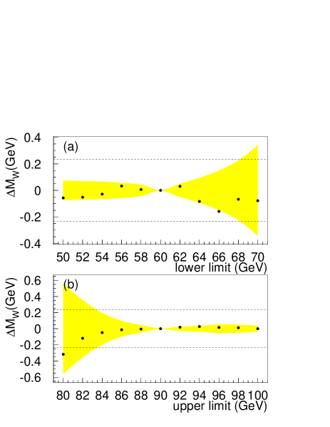
Figure 18: Variation of the fitted $W$ boson mass with (a) the lower edge and (b) the upper edge of the fit window for the transverse mass distribution. The shaded regions and the dashed lines are described in the text.

VI.2 Mass error determination

In addition to the statistical errors determined from the fits, there are systematic errors arising from the uncertainties in all of the parameters that enter in the Monte Carlo production, decay and detector model. These parameters, summarized in Table 6, form a parameter vector $\vec{P}$. The definition and determination of the parameters are described above and in Ref. ccmw1b . The recoil response takes into account the joint effects of two correlated parameters $\alpha_{\rm rec}$ and $\beta_{\rm rec}$. We assign an uncertainty in $M_{W}$ for the uncorrelated errors obtained from the principal axes of the $\alpha_{\rm rec}-\beta_{\rm rec}$ error ellipse ccmw1b . The recoil resolution depends on correlated parameters $s_{\rm rec}$ and $\alpha_{\rm mb}$ ccmw1b , and the $u_{\parallel}$ efficiency depends on correlated parameters $u_{0}$ and $s_{0}$; these correlated pairs are treated similarly to those for the recoil response. The set of production model errors include the parameters due to parton distribution function (PDF) uncertainty, $W$ boson width wwidth , the parameters determining the $W$ boson production $p_{T}$ spectrum, and the parton luminosity function. We take the components of the production model error to be uncorrelated. The PDF error is taken from the deviation of the $W$ boson mass comparing ecmw MRS(A)^′ MRSA , MRSR2 MRSR2 , CTEQ5M CTEQ5M , CTEQ4M CTEQ4M , and CTEQ3M CTEQ3M PDF’s to our standard choice of MRST.

In all, we have identified $N_{P}=21$ parameters that determine the model for the Monte Carlo: the eighteen used in the previous studies and the three new parameters related to the edge electrons ($\widetilde{\alpha}$, $\widetilde{c}$ and $\widetilde{f}$).

Table 6: Parameters $\vec{P}$ used in the $W$ boson mass determination

Parameter	Description
$\alpha$	EM energy response scale for non-edge $e$
$\widetilde{\alpha}$	EM energy response scale for edge $e$
$\delta$	EM response offset
$c$	EM resolution constant for non-edge $e$
$\widetilde{c}$	EM resolution constant for edge $e$
$\widetilde{f}$	fraction of low response $e$ in edge region
$\beta_{\rm cdc}$	drift chamber position scale factor
$\alpha_{\rm rec}$	recoil energy response scale constant
$\beta_{\rm rec}$	recoil energy response scale $Q^{2}$ dependence
$s_{\rm rec}$	recoil energy resolution
$\alpha_{\rm mb}$	recoil energy from added minimum bias events
$\Delta u_{\parallel}$	underlying event energy correction in $e$ window
$u_{0}$	$u_{\parallel}$ cutoff for constant efficiency
$s_{0}$	slope of $u_{\parallel}$ efficiency vs $u_{\parallel}$
$b_{W}$	background to $W$ boson distribution
$r_{\gamma}$	coalescing radius for photon radiation
$2\gamma$	error for 2 $\gamma$ radiation
PDF	error from varying PDF
$\Gamma_{W}$	$W$ boson width
$\beta$	parton luminosity
$g_{2}$	$Q^{2}$ dependence of $W$ boson production

The parameters ${P_{i}}$ are determined from $N_{Y}=32$ auxiliary measurements using several data sets which include the CC and $\widetilde{\rm C}$C $Z$ boson samples, special minimum bias and muon samples for determining drift chamber scales and underlying event properties, and external data sets that are used to constrain the $W$ boson production model. The measurements using these special data sets are denoted ${Y_{I}}$ ($I=1,...~{}N_{Y}$) with uncertainties ${\sigma^{Y}_{I}}$. Each measurement puts constraints on one or more of the parameters $P_{i}$. Measurements ${Y_{I}}$ are related to the parameters ${P_{i}}$ through the functional relation $Y_{I}=F_{I}(\vec{P})$.

We form the $\chi^{2}$ for the set of measurements

$$\chi^{2}=\sum_{I,J=1}^{N_{Y}}{[Y_{I}-F_{I}(\vec{P})](C^{Y}_{IJ})^{-1}[Y_{J}-F_{J}(\vec{P})]\over(\sigma^{Y}_{I}\sigma^{Y}_{J})}~{},$$ (11)

where $C^{Y}_{IJ}=\langle\Delta Y_{I}\Delta Y_{J}\rangle$ is the covariance matrix of the measurements, determined from Monte Carlo calculations. If the deviations of the measurements from their means are taken to be linearly related to the parameters in the region of the $\chi^{2}$ minimum:

$$\Delta Y_{I}=\sum_{j=1}^{N_{P}}{D^{Y}_{Ij}\Delta P_{j}},$$ (12)

where $D^{Y}_{Ij}=\partial F_{I}/\partial P_{j}$, the minimum of the $\chi^{2}$ can be found analytically. The parameter covariance matrix ${C^{P}_{ij}}$ can be then calculated from $C^{Y}_{IJ}$ and the derivatives $D^{Y}_{Ij}$.

This analysis is carried out for the three distinct measurements of $M_{W}$ for the edge electrons ($m_{T}$, $p_{T}(e)$ and $p_{T}(\nu)$). Each measurement depends on the set of parameters, $\vec{P}$, discussed above. For the $N_{M}=3$ separate mass measurements ${m_{\alpha}}$ ($\alpha=1,...N_{M}$), the mass measurement covariance matrix $C^{M}_{\alpha\beta}$ is obtained from

$$C^{M}_{\alpha\beta}=\sum_{k,l=1}^{N_{P}}D^{M}_{\alpha k}C^{P}_{kl}D^{M}_{l\beta},$$ (13)

where $D^{M}_{\alpha j}=\partial m_{\alpha}/\partial P_{j}$. The correlation of the statistical errors is obtained from studies of Monte Carlo ensembles; these correlations are shown in Table 7.

We can fit for the best combined mass value $M_{W}$ by minimizing the $\chi^{2}$ lyons

$$\chi^{2}=\sum_{\alpha,\beta=1}^{N_{M}}(m_{\alpha}-M_{W})H_{\alpha\beta}(m_{\beta}-M_{W}),$$ (14)

where $\mathbf{H}=(\mathbf{C^{M}})^{-1}$. The best fit is given by

$$M_{W}=\bigl{(}\sum_{\alpha,\beta=1}^{N_{M}}H_{\alpha\beta}m_{i}\bigr{)}/\sum_{\alpha,\beta=1}^{N_{M}}H_{\alpha\beta},$$ (15)

with error

$$\sigma_{m}=(\sum_{\alpha,\beta=1}^{N_{M}}H_{\alpha\beta})^{-1/2}.$$ (16)

Table 7: The statistical correlation coefficients for the three measurements of the $W$ boson mass.

	$m_{T}$	$p_{T}(e)$	$p_{T}(\nu)$
$m_{T}$	1	0.669	0.630
$p_{T}(e)$	0.669	1	0.180
$p_{T}(\nu)$	0.630	0.180	1

The resultant $W$ boson mass measurements using electrons in the edge region are

$$M_{W}=80.596\pm 0.234\pm 0.370~{}{\rm GeV}$$ (17)

for the $m_{T}(W)$ fit,

$$M_{W}=80.733\pm 0.263\pm 0.460~{}{\rm GeV}$$ (18)

for the $p_{T}(e)$ fit, and

$$M_{W}=80.511\pm 0.311\pm 0.523~{}{\rm GeV}$$ (19)

for the $p_{T}(\nu)$ fit, where the first error is statistical and the second is systematic. The breakdown of the contributions to the systematic errors is shown in Table 8. The PDF error is taken as the difference on the combined $W$ boson mass between the CTEQ3M and MRST choices, for which $m_{W}$ differs maximally. The combined mass error from this source (not shown in Table 8) is 19 MeV. The errors associated with the broad Gaussian parameters in the edge electron response ($\widetilde{\alpha}$ and $\widetilde{c}$) dominate the systematic errors.

The three measurements of $M_{W}$ are correlated as shown in Table 9; when combined taking these correlations into account, we obtain

$$M_{W}=80.574\pm 0.405~{}{\rm GeV},$$ (20)

with $\chi^{2}=0.61$ for two degrees of freedom.

Table 8: Errors (in MeV) for the three $W$ boson measurements

Source	$m_{T}$	$p_{T}(e)$	$p_{T}(\nu)$
statistics	234	263	311
edge EM scale ($\widetilde{\alpha}$)	265	309	346
CC EM scale ($\alpha$)	128	131	113
CC EM offset ($\delta$)	142	139	145
calorimeter uniformity	10	10	10
CDC scale	38	40	52
backgrounds	10	20	20
CC EM constant term $c$	15	18	2
edge EM constant term ($\widetilde{c}$)	268	344	404
fraction of events ($\widetilde{f}$)	8	14	22
hadronic response	20	16	46
hadronic resolution	25	10	90
$u_{\parallel}$  correction	15	15	20
$u_{\parallel}$  efficiency	2	9	20
parton luminosity	9	11	9
radiative corrections	3	6	$<1$
$2\gamma$	3	6	$<1$
$p_{T}(W)$ spectrum	10	50	25
$W$ boson width	10	10	10

Table 9: The full correlation coefficients for the three measurements of the $W$ boson mass.

	$m_{T}$	$p_{T}(e)$	$p_{T}(\nu)$
$m_{T}$	1	0.90	0.89
$p_{T}(e)$	0.90	1	0.76
$p_{T}(\nu)$	0.89	0.76	1

VII Combination of all DØ $W$ boson mass measurements

The analysis presented here for the edge electrons brings two new ingredients to the DØ $W$ mass measurements. First, the edge electron sample is statistically independent of all other measurements, and thus can be combined to give an improved $M_{W}$ measurement. Second, the added statistics of the $\widetilde{\rm C}$C and $\widetilde{\rm C}$E $Z$ boson samples can be used to refine the knowledge of the electron response parameters for non-edge central calorimeter or end calorimeter electrons. The improved energy scale factors in turn give improved $W$ boson mass precision.

VII.1 Modified non-edge electron $W$ boson mass

Using the $\widetilde{\rm C}$C sample and the same fitting procedure described in Section IV for the $\widetilde{\rm C}$ electrons, we have obtained a scale factor $\alpha=0.9552\pm 0.0023$ for the non-edge electrons. This value can be compared with the previous determination from the CC sample ccmw1b of $\alpha=0.9540\pm 0.0008$. The correlation matrix for CC and $\widetilde{\rm C}$C measurements is calculated in the manner discussed in Section VI.

Similarly, the $\widetilde{\rm C}$E sample can be used to constrain the scale factor $\alpha$ for both end and non-edge central electrons (recall that the central edge electrons contain a fraction $(1-f_{\rm edge})$ of events whose scale factor and resolution are identical to those of the central non-edge electrons). Taking into account the correlations, we obtain $\alpha=0.9559\pm 0.0107$ for electrons in the non-edge region of the central calorimeter and $\alpha=0.9539\pm 0.0085$ for the electrons in the end calorimeter. The latter value can be compared with the previous value ecmw of the end calorimeter electron scale of $0.9518\pm 0.0019$.

Taking the two new measurements of $\alpha$ for the central calorimeter together with the previously determined value, we obtain

$$\alpha=0.9541\pm 0.00075.$$ (21)

This new scale factor is higher than the previous value by $0.0001$, and the error is reduced by 6%. For the end calorimeter, the new combined scale factor is

$$\alpha=0.9519\pm 0.0018,$$ (22)

again higher than the previous value by $0.0001$ with a 5% reduction in error.

In principle, the added data could also improve the precision for the resolution constant term $c$ in the central and end calorimeters, but in practice it does not.

With the new values for the scale factors for the non-edge central calorimeter electrons, we obtain modified results for the non-edge central calorimeter $W$ boson mass:

$$M_{W}=80.438\pm 0.107~{}{\rm GeV},$$ (23)

to be compared with the published value of $M_{W}=80.446\pm 0.108$ GeV ccmw1b . The new end calorimeter electron scale factor gives a modified $W$ boson mass:

$$M_{W}=80.679\pm 0.209~{}{\rm GeV},$$ (24)

to be compared with the published value from the end calorimeters of $M_{W}=80.691\pm 0.227$ GeV ecmw .

With the modified scale factors for C and E electrons, we obtain

$$M_{W}=80.481\pm 0.085~{}{\rm GeV},$$ (25)

with $\chi^{2}=5.5$ (6 degrees of freedom) for all non-edge central and end calorimeter measurements, compared with the previous determination $M_{W}=80.482\pm 0.091$ GeV ecmw .

VII.2 Combined $W$ boson mass from all DØ measurements

With the edge electron mass determinations reported in this paper, there are now ten separate DØ $W$ boson measurements: the Run 1a central calorimeter transverse mass measurement ccmw1a , three Run 1b central calorimeter non-edge measurements ccmw1b (from the transverse mass and electron and neutrino transverse momenta), three Run 1b end calorimeter measurements ecmw , and the three present measurements of the central calorimeter edge electrons. Combining these ten mass measurements using the method outlined in Sec. VI and an expanded set of measurements and parameters to incorporate also the end calorimeter electrons, we obtain a final DØ combined measured value for the $W$ boson mass of

$$M_{W}=80.483\pm 0.084~{}{\rm GeV}$$ (26)

with $\chi^{2}=6.3$ (9 degrees of freedom). This value is to be compared with our previous ecmw combined measurement of $M_{W}=80.482\pm 0.091$ GeV. The edge electrons in the central calorimeter have improved the precision over the previously published results by 7 MeV, or 8%.

VIII Summary

Using a sample of electrons which impact upon the 10% of a central calorimeter module closest to either module edge in azimuth, we have made a new measurement of the $W$ boson mass, and have refined our knowledge of the energy scale for previously used electrons that are in the interior 80% of the central calorimeter modules or are in the end calorimeters. Adding the new measurement using the edge electrons gives the final combined result

$$M_{W}=80.483\pm 0.084~{}{\rm GeV}~{}~{}~{}({\rm D\O}).$$

Combining the new DØ $W$ boson mass value reported here with the CDF cdfmw and UA2 ua2 measurements, taking into account the updated correlated systematic errors for the three experiments due to parton distribution function uncertainties and multiple photon radiation gives tevavg

$$M_{W}=80.454\pm 0.059~{}{\rm GeV}~{}~{}~{}(p\overline{p}).$$

This is an improvement over the previous measurement from hadron colliders of $M_{W}=80.452\pm 0.062$ GeV kotwal . Further combining with the LEP experiments’ preliminary measurement $M_{W}=80.450\pm 0.039$ GeV ewwkgp , we find the world average $W$ boson mass from direct measurements to be tevavg

$$M_{W}=80.451\pm 0.033~{}{\rm GeV}~{}~{}~{}({\rm world}).$$

The edge electrons used in this analysis represent a 14% increase in the central calorimeter $W$ boson sample, and an 18% increase in the total $Z$ boson sample. The larger sample sizes should be of use for all subsequent studies of vector bosons in DØ.

References

- (1)
- (2) Also at University of Zurich, Zurich, Switzerland.
- (3) Also at Institute of Nuclear Physics, Krakow, Poland.
- (4) S. L. Glashow, Nucl. Phys. 22, 579 (1961); S. Weinberg, Phys. Rev. Lett. 19, 1264 (1967); A. Salam, Proceedings of the 8th Nobel Symposium, edited by N. Svartholm (Almqvist and Wiksells, Stockholm, 1968), p. 367.
- (5) LEP Electroweak Working Group, CERN-EP/2001-098, Dec. 17, 2001 (unpublished); http://lepewwg.web.cern.ch/LEPEWWG/ and hep-ex/0112021.
- (6) B. Abbott et al. (DØ Collaboration), Phys. Rev. D 62, 092006 (2000).
- (7) B. Abbott et al. (DØ Collaboration), Phys. Rev. D 58, 092003 (1998).
- (8) B. Abbott et al. (DØ Collaboration), Phys. Rev. D 58, 012002 (1998).
- (9) T. Affolder et al. (CDF Collaboration), Phys. Rev. D 64, 052001 (2001).
- (10) R. Barate et al. (ALEPH Collaboration), Eur. Phys. J. C 17, 241 (2000).
- (11) P. Abreu et al. (DELPHI Collaboration), Phys. Lett. B 511, 159 (2001).
- (12) M. Acciarri et al. (L3 Collaboration), Phys. Lett. B 454, 386 (1999).
- (13) K. Ackerstaaff et al. (OPAL Collaboration), Phys. Lett. B 453, 138 (1999).
- (14) G. P. Zeller et al. (NuTEV Collaboration), Phys. Rev. Letters, 88, 091802 (2002).
- (15) B. Abbott et al. (DØ Collaboration), Phys. Rev. D 60, 052001 (1999); F. Abe et al. (CDF Collaboration), Phys. Rev. Lett. 82, 271 (1999), erratum ibid 82, 2808 (1999); the averaging of DØ and CDF results is found in L. Demortier et al., Fermilab-TM-2084, 1999 (unpublished).
- (16) Y. Kulik, Ph.D. thesis, State University of New York at Stony Brook, 2001 (unpublished); http://www-d0.fnal.gov/results/publications_talks/thesis/ kulik/thesis.ps.
- (17) S. Abachi et al. (DØ Collaboration), Nucl. Instrum. Methods Phys. Res. A 338, 185 (1994).
- (18) S. Abachi et al. (DØ Collaboration), Phys. Rev. D 52, 4877 (1995).
- (19) B. Abbott et al. (DØ Collaboration), Phys. Rev. D 62, 092006 (2000).
- (20) G. A. Ladinsky and C. P. Yuan, Phys. Rev. D 50, 4239 (1994).
- (21) A. D. Martin, R. G. Roberts, W. J. Stirling and R. S. Thorne, Eur. Phys. J. C 4, 463 (1998).
- (22) F. A. Behrends and R. Kleiss, Z. Phys. C 27, 365 (1985); F. A. Behrends, R. Kleiss, J. P. Revol and J. P. Vialle; ibid, C 27, 155 (1985).
- (23) F. Carminati et al., CERN Program Library W5013, 1991 (unpublished).
- (24) We use the measured boson width GeV; S. Abachi et al. (DØ Collaboration), Phys. Rev. Letters 75, 1456 (1995).
- (25) A. D. Martin, W. J. Stirling and R. G. Roberts, Phys. Rev. D 50, 6743 (1994); ibid D 51, 4756 (1995).
- (26) A. D. Martin, R. G. Roberts and W. J. Stirling, Phys. Lett. B 387, 419 (1996).
- (27) H. L. Lai et al., hep-ph/9903282 (unpublished).
- (28) H. L. Lai et al., Phys. Rev. D 55, 1280 (1997).
- (29) H. L. Lai et al., Phys. Rev. D 51, 4763 (1995).
- (30) L. Lyons, D. Gibaut, P. Clifford, Nucl. Instrum. Methods Phys. Res. A 270, 110 (1988).
- (31) J. Alitti et al. (UA2 Collaboration), Phys. Lett. B 276, 354 (1992).
- (32) “Combination of CDF and DØ results on Boson Mass and Width”, CDF and DØ collaborations, Fermilab-FN-716 (2002) (unpublished).
- (33) R. M. Thurman-Keup, A. V. Kotwal, M. Tecchio, A. Byon-Wagner, Rev. Mod. Physics 73, 267 (2001).