Study of the Decay $\phi\rightarrow\mbox{$\pi^{0}$}\mbox{$\pi^{0}$}\gamma$ with the KLOE Detector

Abstract

We have measured the branching ratio BR($\phi\rightarrow\mbox{$\pi^{0}$}\mbox{$\pi^{0}$}\gamma$) with the KLOE detector using a sample of $\sim$$5\times 10^{7}$ $\phi$ decays. $\phi$ mesons are produced at DAΦNE, the Frascati $\phi$-factory. We find BR($\phi$$\rightarrow$$\pi^{0}$$\pi^{0}$$\gamma$)= $(1.09\pm 0.03_{\rm stat}\pm 0.05_{\rm syst})\times 10^{-4}$. We fit the two–pion mass spectrum to models to disentangle contributions from various sources.

, , , , , , , , , , , , , , , , , , , , , , , , , , , , , , , , , , , , , , , , , , , , , , , , , , , , , , , , , , , , , , , , , , , , , , , , , , , , , , , , , , , , , , , , , , , , , , , , , , , , , , , , , , , ,

The decay $\phi\rightarrow\mbox{$\pi^{0}$}\mbox{$\pi^{0}$}\gamma$ was first observed in 1998 [1]. Only two experiments have measured its rate [2, 3]. The measured rate is too large if $\phi$$\rightarrow$$f_{0}$(980)$\gamma$, with $f_{0}\rightarrow\mbox{$\pi^{0}$}\mbox{$\pi^{0}$}$, were the dominating contribution and $f_{0}$(980) is interpreted as a $q\overline{q}$ scalar state [4, 5]. Possible explanations for the $f_{0}$ are: ordinary $q\overline{q}$ meson, $q\overline{q}q\overline{q}$ state, $K\overline{K}$ molecule [6, 7, 8, 4]. Similar considerations apply also to the $a_{0}$(980) meson. The decay $\phi\rightarrow\mbox{$\pi^{0}$}\mbox{$\pi^{0}$}\gamma$ can clarify this situation since both the branching ratio and the line shape depend on the structure of the $f_{0}$. We present in the following a study of the decay $\phi\rightarrow\mbox{$\pi^{0}$}\mbox{$\pi^{0}$}\gamma$ performed with the KLOE detector [9] at DAΦNE [10], an $e^{+}e^{-}$ collider which operates at a center of mass energy $W$=$M_{\phi}\sim 1020$ MeV. Data were collected in the year 2000 for an integrated luminosity $\mbox{$L_{\rm int}$}\!\sim\!16$ pb^-1, corresponding to around $5\times 10^{7}$ $\phi$-meson decays.

The KLOE detector consists of a large cylindrical drift chamber, DC, surrounded by a lead-scintillating fiber electromagnetic calorimeter, EMC. A superconducting coil around the EMC provides a 0.52 T field. The drift chamber [11], 4 m in diameter and 3.3 m long, has 12,582 all-stereo tungsten sense wires and 37,746 aluminum field wires. The chamber shell is made of carbon fiber-epoxy composite and the gas used is a 90% helium, 10% isobutane mixture. These features maximize transparency to photons and reduce $\mbox{$K_{L}$}\rightarrow\mbox{$K_{S}$}$ regeneration and multiple scattering. The position resolutions are $\sigma_{xy}$$\sim$150 $\mu$m and $\sigma_{z}$$\sim$ 2 mm. The momentum resolution is $\sigma(p_{\perp})/p_{\perp}\approx 0.4\%$. Vertices are reconstructed with a spatial resolution of $\sim$3 mm. The calorimeter [12] is divided into a barrel and two endcaps, for a total of 88 modules, and covers 98% of the solid angle. The modules are read out at both ends by photomultipliers; the readout granularity is $\sim$4.4$\times$4.4 cm², for a total of 2440 cells. The arrival times of particles and the positions in three dimensions of the energy deposits are obtained from the signals collected at the two ends. Cells close in time and space are grouped into a calorimeter cluster. The cluster energy $E$ is the sum of the cell energies. The cluster time $T$ and position $\vec{R}$ are energy weighted averages. Energy and time resolutions are $\sigma_{E}/E=5.7\%/\sqrt{E\ {\rm(GeV)}}$ and $\sigma_{t}=57\ {\rm ps}/\sqrt{E\ {\rm(GeV)}}\oplus 50\ {\rm ps}$, respectively. The KLOE trigger [13] uses calorimeter and chamber information. For this analysis only the calorimeter signals are relevant. Two energy deposits with $E>50$ MeV for the barrel and $E>150$ MeV for the endcaps are required.

Prompt photons are identified as neutral particles with $\beta=1$ originated at the interaction point requiring $|T-R/c|<{\rm min}(5\sigma_{T},2\ {\rm ns})$, where $T$ is the photon flight time and $R$ the path length; $\sigma_{T}$ includes also the contribution of the bunch length jitter. The photon detection efficiency is $\sim 90\%$ for $E_{\gamma}$=20 MeV, and reaches 100% above 70 MeV. The sample selected by the timing requirement contains a $<1.8\%$ contamination due to accidental clusters from machine background.

Two amplitudes contribute to $\phi\rightarrow\mbox{$\pi^{0}$}\mbox{$\pi^{0}$}\gamma$: $\phi$$\rightarrow$$S$$\gamma$, $S$$\rightarrow$$\pi^{0}$$\pi^{0}$ ($S\gamma$) and $\phi$$\rightarrow$$\rho^{0}$$\pi^{0}$, $\rho^{0}$$\rightarrow$$\pi^{0}$$\gamma$ ($\rho\pi$) where $S$ is a scalar meson. The event selection criteria of the $\phi\rightarrow\mbox{$\pi^{0}$}\mbox{$\pi^{0}$}\gamma$ decays ($\pi\pi\gamma$) have been designed to give similar efficiencies for both processes. The first step, requiring five prompt photons with $E_{\gamma}\!\geq$7 MeV and $\theta\geq\theta_{\rm min}=23^{\circ}$, reduces the sample to 124,575 events. The background due to $\phi$$\rightarrow$$K_{S}$$K_{L}$  is removed requiring that $E_{\rm tot}=\sum_{5}E_{\gamma,i}$ and $\vec{p}_{\rm tot}=\sum_{5}\vec{p}_{\gamma,i}$ satisfy $E_{\rm tot}\!>$800 MeV and $|\vec{p}_{\rm tot}|\!<$200 MeV/c. We are left with 15,825 events. Other reactions which give rise to background are: $e^{+}e^{-}$$\rightarrow$$\omega$$\pi^{0}$$\rightarrow$$\pi^{0}$$\pi^{0}$$\gamma$ ($\omega\pi$), $\phi$$\rightarrow$$\eta$$\pi^{0}$$\gamma$$\rightarrow$5$\gamma$ ($\eta$$\pi$$\gamma$) and $\phi$$\rightarrow$$\eta$$\gamma$$\rightarrow$3$\pi^{0}$$\gamma$ ($\eta\gamma$) with 2 undetected photons.

A kinematic fit (Fit1) requiring overall energy and momentum conservation improves the energy resolution to $3\%$. Photons are assigned to $\pi^{0}$’s by minimizing a test $\chi^{2}$-function for both the $\pi\pi\gamma$ and $\omega\pi$ cases. For the $\omega\pi$ case we also require $M_{\pi\gamma}$ to be consistent with $M_{\omega}$. The correct combination is found by this procedure 89%, 96% of the time for the $\pi\pi\gamma$, $\omega\pi$ case respectively. Good agreement is found with the Monte Carlo simulation, MC, for the distributions of the $\chi^{2}$ and of the invariant masses. A second fit (Fit2) requires the masses of $\gamma$$\gamma$ pairs to equal $M_{\pi}$.

The $\mbox{$e^{+}$}\mbox{$e^{-}$}\rightarrow\omega\mbox{$\pi^{0}$}\rightarrow\mbox{$\pi^{0}$}\mbox{$\pi^{0}$}\gamma$ background is reduced rejecting the events satisfying $\chi^{2}/{\rm ndf}\leq 3$ and $\Delta M_{\pi\gamma}=|M_{\pi\gamma}-M_{\omega}|\leq 3\,\sigma_{\omega}$ using Fit2 in the $\omega\pi$ hypothesis. Data and MC are in good agreement (Fig. 1.a-b).

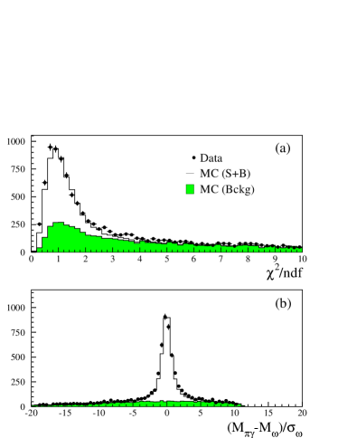
Figure 1: Data–MC comparison for $\omega\pi$ events: (a) $\chi^{2}$/ndf and (b) $\Delta M_{\pi\gamma}/\sigma_{\omega}$.

The $\phi\rightarrow\mbox{$\pi^{0}$}\mbox{$\pi^{0}$}\gamma$ events must then satisfy $\chi^{2}/{\rm ndf}\leq 3$ for Fit2 in the $\pi\pi\gamma$ hypothesis. We also require $\Delta M_{\gamma\gamma}=|M_{\gamma\gamma}-M_{\pi}|\leq 5\,\sigma_{\pi}$ using the photon momenta of Fit1. The efficiency for the identification of the signal is evaluated applying the whole analysis chain to a sample of simulated $\phi$$\rightarrow$$S$$\gamma$, $S$$\rightarrow$$\pi^{0}$$\pi^{0}$ events with a $\pi^{0}$$\pi^{0}$ mass ($m$) spectrum consistent with the data. We use the symbol $M_{\pi\pi}$ to denote the reconstructed value of $m$. The selection efficiency as a function of $M_{\pi\pi}$ is shown in Fig.  2. The average over the whole mass spectrum is $\epsilon_{\pi\pi\gamma}=41.6\%$. A similar efficiency function is obtained for the process $\phi\rightarrow\rho^{0}\mbox{$\pi^{0}$}$ with $\rho^{0}\rightarrow\mbox{$\pi^{0}$}\gamma$.

Figure 2: Efficiency vs $\pi^{0}$$\pi^{0}$ invariant mass for $\phi\rightarrow\mbox{$\pi^{0}$}\mbox{$\pi^{0}$}\gamma$ events.

Fig. 3 shows various distributions for the 3102 events surviving the selection together with MC predictions. The angular distributions prove that $S\gamma$ is the dominant process.

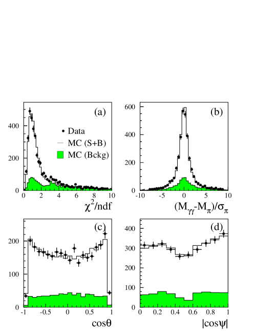
Figure 3: Data–MC comparison for $\phi\rightarrow\mbox{$\pi^{0}$}\mbox{$\pi^{0}$}\gamma$ events after $\omega\pi$ rejection: (a) $\chi^{2}$/ndf; (b) $(M_{\gamma\gamma}-M_{\pi})/\sigma_{\pi}$ with $\chi^{2}/{\rm ndf}\leq 3$; (c, d) angular distributions with all analysis cuts applied. $\theta$ is the polar angle of the radiative photon, $\psi$ is the angle between the radiative photon and $\pi^{0}$ in the $\pi^{0}$$\pi^{0}$ rest frame.

The rejection factors and the expected number of events for the background processes are listed in Tab. 1 [14, 15, 16].

Table 1: Background channels for $\phi\rightarrow\mbox{$\pi^{0}$}\mbox{$\pi^{0}$}\gamma$.

Process	Rejection Factor	Expected events
$\mbox{$e^{+}$}\mbox{$e^{-}$}\rightarrow\omega\mbox{$\pi^{0}$}\rightarrow\mbox{$\pi^{0}$}\mbox{$\pi^{0}$}\gamma$	8.7	$339\pm 24$
$\phi\rightarrow\eta\mbox{$\pi^{0}$}\gamma\rightarrow\gamma\gamma\mbox{$\pi^{0}$}\gamma$	4.0	$166\pm 16$
$\phi\rightarrow\eta\gamma\rightarrow\mbox{$\pi^{0}$}\mbox{$\pi^{0}$}\mbox{$\pi^{0}$}\gamma$	$5.9\times 10^{3}$	$159\pm 12$

After subtracting the background 2438$\pm$61 $\phi\rightarrow\mbox{$\pi^{0}$}\mbox{$\pi^{0}$}\gamma$ events remain. Their $M_{\pi\pi}$ spectrum is shown in Fig. 4.

The $\phi\rightarrow\mbox{$\pi^{0}$}\mbox{$\pi^{0}$}\gamma$ branching ratio, BR, is obtained normalizing the number of events after background subtraction, $N-B$, to the $\phi$ cross section, $\sigma(\phi)$, to the selection efficiency and to $L_{\rm int}$:

$$\mbox{BR}(\mbox{$\phi\rightarrow\mbox{$\pi^{0}$}\mbox{$\pi^{0}$}\gamma$})=\frac{N-B}{\epsilon_{\pi\pi\gamma}}\>\frac{1}{\sigma(\phi)\,\mbox{$L_{\rm int}$}}$$ (1)

The luminosity is measured using large angle Bhabha scattering events. The measurement of $\sigma(\phi)$ is obtained from the $\phi\rightarrow\eta\gamma\rightarrow\gamma\gamma\gamma$ decay in the same sample [15]. We obtain:

$$\mbox{BR}(\mbox{$\phi\rightarrow\mbox{$\pi^{0}$}\mbox{$\pi^{0}$}\gamma$})=(1.08\pm 0.03_{\rm stat}\pm 0.03_{\rm syst}\pm 0.04_{\rm norm})\times 10^{-4}.$$ (2)

The contributions to the uncertainties are listed in Tab. 2. Details can be found in Ref. [16].

Table 2: Uncertainties on BR($\phi\rightarrow\mbox{$\pi^{0}$}\mbox{$\pi^{0}$}\gamma$).

Source	Relative error
Statistics	2.5%
Background	1.3%
Event counting	2.3%
Normalization	3.7%
Total	5.2%

In order to disentagle the contributions of the various processes and to determine the normalized differential decay rate, ${\rm d\hskip 0.85358pt}\mbox{BR}/{\rm d\hskip 0.85358pt}m=(1/\Gamma){\rm d\hskip 0.85358pt}\Gamma/{\rm d\hskip 0.85358pt}m$, we fit the data to a mass spectrum $f(m)$. This spectrum is taken as the sum of $S\gamma$, $\rho\pi$ and interference term, $f(m)=f_{S\gamma}(m)+f_{\rho\pi}(m)+f_{\rm int}(m)$. The scalar term is [17]:

$$f_{S\gamma}(m)=\frac{2\,m^{2}}{\pi}\>\frac{\Gamma_{\phi S\gamma}\Gamma_{S\pi^{0}\pi^{0}}}{|D_{S}|^{2}}\>\frac{1}{\Gamma_{\phi}}.$$ (3)

The $\phi$$\rightarrow$$S$$\gamma$ process is estimated by means of a $K^{+}K^{-}$ loop for the $f_{0}$:

$$\Gamma_{\phi f\!_{0}\gamma}(m)=\frac{g^{2}_{f\!_{0}K^{+}K^{-}}g^{2}_{\phi K^{+}K^{-}}}{12\pi}\>\frac{|g(m)|^{2}}{M_{\phi}^{2}}\>\left(\frac{M^{2}_{\phi}-m^{2}}{2M_{\phi}}\right),$$ (4)

where $g_{\phi K^{+}K^{-}}$ and $g_{f\!_{0}K^{+}K^{-}}$ are the couplings and $g(m)$ is the loop integral function.

A recent measurement [18] reports the existence of a scalar $\sigma$ with $M_{\sigma}=(478^{+24}_{-23}\pm 17)$ MeV and $\Gamma_{\sigma}=(324^{+42}_{-40}\pm 21)$ MeV. If we include the contribution of this meson, its decay rate is given by [19]:

$$\Gamma_{\phi\sigma\gamma}(m)=\frac{e^{2}\,g^{2}_{\phi\sigma\gamma}}{12\pi}\>\frac{1}{M_{\phi}^{2}}\>\left(\frac{M^{2}_{\phi}-m^{2}}{2M_{\phi}}\right)^{3}.$$ (5)

where $g_{\phi\sigma\gamma}$ is a point-like $\phi\sigma\gamma$ coupling.

Finally, $\Gamma_{S\pi^{0}\pi^{0}}$ is related to $\Gamma_{S\pi^{+}\pi^{-}}$ by:

$$\Gamma_{S\pi^{0}\pi^{0}}(m)=\frac{1}{2}\,\Gamma_{S\pi^{+}\pi^{-}}(m)=\frac{g^{2}_{S\pi^{+}\pi^{-}}}{32\,\pi\,m}\,\sqrt{1-\frac{4M_{\pi}^{2}}{m^{2}}}\ .$$ (6)

For the inverse propagator, $D_{S}$, we use the formula with finite width corrections [17] for the $f_{0}$ and a Breit Wigner for the $\sigma$. The parametrization of Ref. [20] has been used for the $\rho\pi$ and the interference term.

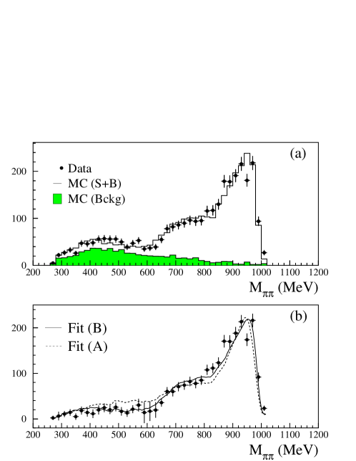
Figure 4: Observed spectrum of $\pi^{0}$$\pi^{0}$ invariant mass before (a) and after (b) background subtraction.

The observed mass spectrum $S_{\rm obs}(\mbox{$M_{\pi\pi}$})$ is fit folding into the theoretical shape experimental efficiency and resolution after proper normalization for $\sigma(\phi)$ and $L_{\rm int}$. Two different fits have been performed varying $f_{S\gamma}(m)$: in Fit (A) only the $f_{0}$ contribution is considered while in Fit (B) we also include the contribution of the $\sigma$ meson. The mass and width of the $\sigma$ were fixed to their central values. If the normalization of the $\rho\pi$ term is left free during fitting, its contribution and the associated interference terms turn out to be negligibly small. When $\mbox{BR}(\phi\rightarrow\rho^{0}\mbox{$\pi^{0}$}\rightarrow\mbox{$\pi^{0}$}\mbox{$\pi^{0}$}\gamma)$ is fixed at $1.8\cdot 10^{-5}$ as in Ref. [20], the $\chi^{2}$/ndf increases by more than a factor of 2. The fits without the $\rho\pi$ contribution are shown superimposed over the raw spectrum in Fig. 4.b.

The result of the fits are listed in Tab. 3.

Table 3: Fit results using $f_{0}$ only, Fit (A), and including the $\sigma$, Fit (B).

	Fit (A)	Fit (B)
$\chi^{2}/{\rm ndf}$	$109.53/34$	$43.15/33$
$M\!\mbox{${}_{f\!_{0}}$}$ (MeV)	$962\pm 4$	$973\pm 1$
$g^{2}_{f\!_{0}K^{+}K^{-}}/(4\pi)$ (GeV2)	$1.29\pm 0.14$	$2.79\pm 0.12$
$g^{2}_{f\!_{0}K^{+}K^{-}}/g^{2}_{f\!_{0}\pi^{+}\pi^{-}}$	$3.22\pm 0.29$	$4.00\pm 0.14$
$g_{\phi\sigma\gamma}$	—	$0.060\pm 0.008$

In Fit (A) we use as free parameters $M\!\mbox{${}_{f\!_{0}}$}$, $g^{2}_{f\!_{0}K^{+}K^{-}}$ and the ratio $g^{2}_{f\!_{0}K^{+}K^{-}}/g^{2}_{f\!_{0}\pi^{+}\pi^{-}}$. The fit gives a large $\chi^{2}$/ndf; integrating the theoretical spectrum a value $\mbox{BR}(\mbox{$\phi\rightarrow f\!_{0}\gamma$}\rightarrow\mbox{$\pi^{0}$}\mbox{$\pi^{0}$}\gamma)=(1.11\pm 0.06_{\rm stat+syst})\times 10^{-4}$ is obtained.

A much better agreement with data is given by Fit (B), where we add as a free parameter also the coupling $g_{\phi\sigma\gamma}$. The negative interference between the $f_{0}$ and $\sigma$ amplitudes results in the observed decrease of the $\mbox{$\pi^{0}$}\mbox{$\pi^{0}$}\gamma$ yield below 700 MeV. Integrating over the theoretical $\sigma$ and $f_{0}$ curves we obtain $\mbox{BR}(\phi\rightarrow\sigma\gamma\rightarrow\mbox{$\pi^{0}$}\mbox{$\pi^{0}$}\gamma)=(0.28\pm 0.04_{\rm stat+syst})\times 10^{-4}$ and $\mbox{BR}(\mbox{$\phi\rightarrow f\!_{0}\gamma$}\rightarrow\mbox{$\pi^{0}$}\mbox{$\pi^{0}$}\gamma)=(1.49\pm 0.07_{\rm stat+syst})\times 10^{-4}$. Multiplying the latter BR by a factor of 3 to account for $f_{0}\rightarrow\mbox{$\pi^{+}$}\mbox{$\pi^{-}$}$ decay, the $\mbox{BR}(\mbox{$\phi\rightarrow f\!_{0}\gamma$})$ is determined to be:

$$\mbox{BR}(\mbox{$\phi\rightarrow f\!_{0}\gamma$})=(4.47\pm 0.21_{\rm stat+syst})\cdot 10^{-4}.$$ (7)

The values of the coupling constants from Fit (B) are in agreement with those reported by the SND and CMD-2 experiments [2, 3]. The coupling constants differ from the WA102 result on $f_{0}$ production in central $pp$ collisions ($g^{2}_{f\!_{0}K^{+}K^{-}}/g^{2}_{f\!_{0}\pi^{+}\pi^{-}}=g_{K}/1.33\,g_{\pi}=1.63\pm 0.46$) [21] and from those obtained when the $f_{0}$ is produced in $D_{s}^{+}\rightarrow\mbox{$\pi^{+}$}\mbox{$\pi^{-}$}\mbox{$\pi^{+}$}$ decays [22], where $g_{K}$ is consistent with zero.

In order to allow a detailed comparison with other experiments and theoretical models, we have unfolded $S_{\rm obs}(\mbox{$M_{\pi\pi}$})$. For each reconstructed mass bin, the ratio between the theoretical and the smeared function, $SF(\mbox{$M_{\pi\pi}$})$, is calculated. The ${\rm d\hskip 0.85358pt}\mbox{BR}/{\rm d\hskip 0.85358pt}m$ is then given by:

$$\frac{{\rm d\hskip 0.85358pt}\mbox{BR}}{{\rm d\hskip 0.85358pt}m}=\frac{S_{\rm obs}(\mbox{$M_{\pi\pi}$})}{SF(\mbox{$M_{\pi\pi}$})}\>\frac{1}{\mbox{$L_{\rm int}$}\times\sigma(\phi)\times\Delta\mbox{$M_{\pi\pi}$}}$$ (8)

The value of ${\rm d\hskip 0.85358pt}\mbox{BR}/{\rm d\hskip 0.85358pt}m$ as a function of $m$ is given in Tab. 4 and shown in Fig. 5. Integrating over the whole mass range we obtain:

$$\mbox{BR}(\mbox{$\phi\rightarrow\mbox{$\pi^{0}$}\mbox{$\pi^{0}$}\gamma$})=(1.09\pm 0.03_{\rm stat}\pm 0.03_{\rm syst}\pm 0.04_{\rm norm})\times 10^{-4}.$$ (9)

which well compares with the result obtained correcting for the average selection efficiency (Eq. 2). If we limit the integration to the $f_{0}$ dominated region, above 700 MeV, we get:

 

BR $${{}(\mbox{$\phi\rightarrow\mbox{$\pi^{0}$}\mbox{$\pi^{0}$}\gamma$};\>m>700\ {\rm MeV})=}$$

 

which is in agreement with our previous measurement in the same mass range [23].

Figure 5: ${\rm d\hskip 0.85358pt}\mbox{BR}/{\rm d\hskip 0.85358pt}m$ as a function of $m$. Fit (B) is shown as a solid line; individual contributions are also shown.

Table 4: Differential BR for $\phi\rightarrow\mbox{$\pi^{0}$}\mbox{$\pi^{0}$}\gamma$. $m$ is expressed in MeV while ${\rm d\hskip 0.85358pt}{\rm BR}/{\rm d\hskip 0.85358pt}m$ is in units of $10^{8}\,{\rm MeV}^{-1}$. The errors listed are the total uncertainties.

$m$	$\frac{d{\rm BR}}{dm}$	$m$	$\frac{d{\rm BR}}{dm}$
1290	$2.0\pm 2.9$	1670	$11.2\pm 1.9$
1310	$2.2\pm 1.4$	1690	$11.0\pm 1.9$
1330	$3.0\pm 1.5$	1710	$12.5\pm 1.9$
1350	$0.9\pm 1.3$	1730	$14.0\pm 2.0$
1370	$2.9\pm 1.4$	1750	$17.3\pm 2.3$
1390	$2.2\pm 1.3$	1770	$17.0\pm 2.4$
1410	$1.4\pm 1.1$	1790	$19.4\pm 2.5$
1430	$1.8\pm 1.0$	1810	$27.4\pm 3.1$
1450	$1.9\pm 0.8$	1830	$29.2\pm 3.2$
1470	$1.1\pm 0.5$	1850	$30.6\pm 3.2$
1490	$0.5\pm 0.2$	1870	$41.7\pm 3.8$
1510	$0.2\pm 0.1$	1890	$39.6\pm 3.6$
1530	$0.3\pm 0.2$	1910	$44.6\pm 3.8$
1550	$1.3\pm 0.5$	1930	$53.6\pm 4.4$
1570	$3.3\pm 1.5$	1950	$47.2\pm 4.3$
1590	$2.1\pm 3.6$	1970	$64.7\pm 5.3$
1610	$3.7\pm 4.7$	1990	$22.0\pm 2.5$
1630	$4.2\pm 3.7$	1010	$\hphantom{1}0.2\pm 0.1$
1650	$7.0\pm 1.7$

In a separate paper [14], we present a measurement of $\mbox{BR}(\phi\rightarrow a_{0}\gamma$), together with a discussion of the implications of $f_{0}$ and $a_{0}$ results.

References

[1]
M.N. Achasov et al., Phys. Lett. B 440 (1998) 442.
[2]
M.N. Achasov et al., Phys. Lett. B 485 (2000) 349.
[3]
R.R. Akhmetshin et al., Phys. Lett. B 462 (1999) 380.
[4]
F.E. Close, N. Isgur and S. Kumano, Nucl. Phys. B 389 (1993) 513.
[5]
N. Brown and F.E. Close, “Second DANE Physics Handbook”,
Ed. L. Maiani, G. Pancheri and N. Paver, Vol. 2 (1995) 649.
[6]
N.A. Törnqvist, Phys. Rev. Lett. 49 (1982) 624.
[7]
R.L. Jaffe, Phys. Rev. D 15 (1997) 267.
[8]
J. Weinstein and N. Isgur, Phys. Rev. Lett. 48 (1982) 659.
[9]
KLOE Collaboration, LNF-92/019 (IR) (1992) and LNF-93/002 (IR) (1993).
[10]
S. Guiducci et al., Proc. of the 2001 Particle Accelerator Conference
(Chicago, Illinois, USA), P. Lucas S. Webber Eds., 2001, 353.
[11]
KLOE Collaboration, M. Adinolfi et al.,
LNF Preprint LNF-01/016 (IR) (2001), accepted by Nucl. Inst. and Meth.
[12]
KLOE Collaboration, M. Adinolfi et al.,
Nucl. Inst. and Meth. A 482 (2002) 363.
[13]
KLOE Collaboration, M. Adinolfi et al.,
LNF Preprint LNF-02/002 (P) (2002), submitted to Nucl. Inst. and Meth.
[14]
KLOE Collaboration, A. Aloisio et al., hep-ex/0204012 (2002),
submitted to Phys. Lett. B.
[15]
S. Giovannella and S. Miscetti, KLOE Note 177 (2002).
[16]
S. Giovannella and S. Miscetti, KLOE Note 178 (2002).
[17]
N.N. Achasov and V.N. Ivanchenko, Nucl. Phys. B 315 (1989) 465.
[18]
E.M. Aitala et al., Phys. Rev. Lett. 86 (2001) 770.
[19]
A. Gokalp and O. Yilmaz, Phys. Rev. D 64 (2001) 053017
and private communication.
[20]
N.N. Achasov and V.V. Gubin, Phys. Rev. D 63 (2001) 094007.
[21]
D. Barberis et al., Phys. Lett. B 462 (1999) 462;
F.E. Close A. Kirk, Phys. Lett. B 515 (2001) 13.
[22]
E.M. Aitala et al., Phys. Rev. Lett. 86 (2001) 765.
[23]
KLOE Collaboration, A. Aloisio et al., hep-ex/0107024 (2001).