Measurement of the $b$-Quark Fragmentation
Function in $Z^{0}$ Decays^∗

ABSTRACT

We present a measurement of the $b$-quark inclusive fragmentation function in $Z^{0}$ decays using a novel kinematic $B$-hadron energy reconstruction technique. The measurement was performed using 350,000 hadronic $Z^{0}$ events recorded in the SLD experiment at SLAC between 1997 and 1998. The small and stable SLC beam spot and the CCD-based vertex detector were used to reconstruct $B$-decay vertices with high efficiency and purity, and to provide precise measurements of the kinematic quantities used in this technique. We measured the $B$ energy with good efficiency and resolution over the full kinematic range. We compared the scaled $B$-hadron energy distribution with models of $b$-quark fragmentation and with several ad hocfunctional forms. A number of models and functions are excluded by the data. The average scaled energy of weakly-decaying $B$ hadrons was measured to be $<x_{b}>$ = 0.709 $\pm$ 0.003 (stat) $\pm$ 0.003 (syst) $\pm$ 0.002 (model).

Submitted to Physical Review D

^∗ Work supported by Department of Energy contract DE-AC03-76SF00515 (SLAC).

1 Introduction

The production of heavy hadrons ($H$) in $e^{+}e^{-}$annihilation provides a laboratory for the study of heavy-quark ($Q$) jet fragmentation. This is commonly characterised in terms of the observable $x_{H}$ $\equiv$ $2E_{H}/\sqrt{s}$, where $E_{H}$ is the energy of a $B$ or $D$ hadron containing a $b$ or $c$ quark, respectively, and $\sqrt{s}$ is the c.m. energy. In contrast to light-quark jet fragmentation one expects [2] the distribution of $x_{H}$, $D(x_{H})$, to peak at an $x_{H}$-value significantly above 0. Since the hadronisation process is intrinsically non-perturbative $D(x_{H})$ cannot be calculated directly using perturbative Quantum Chromodynamics (QCD). However, the distribution of the closely-related variable $x_{Q}$ $\equiv$ 2$E_{Q}/\sqrt{s}$ can be calculated perturbatively [3, 4, 5, 6] and related, via model-dependent assumptions, to the observable quantity $D(x_{H})$; a number of such models of heavy-quark fragmentation have been proposed [7, 8, 9, 10]. Measurements of $D(x_{H})$ thus serve to constrain both perturbative QCD and the model predictions. Furthermore, the measurement of $D(x_{H})$ at different c.m. energies can be used to test QCD evolution, and comparison of $D(x_{B})$ with $D(x_{D})$ can be used to test heavy-quark symmetry [11]. Finally, the uncertainty on the forms of $D(x_{D})$ and $D(x_{B})$ must be taken into account in studies of the production and decay of heavy quarks, see eg. [12]; more accurate measurements of these forms will allow increased precision in tests of the electroweak heavy-quark sector.

We have measured the inclusive weakly-decaying $B$-hadron scaled energy distribution $D(x_{B})$ in $Z^{0}$ decays. Earlier studies [13] used the momentum spectrum of the lepton from semi-leptonic $B$ decays to constrain the mean value $<x_{B}>$ and found it to be approximately $0.70$; this is in agreement with the results of similar studies at $\sqrt{s}$ = 29 and 35 GeV [14]. In more recent analyses [15, 16, 17] $D(x_{B})$ has been measured by reconstructing $B$ hadrons via their $B$ $\rightarrow$$DlX$ decay mode. In this case the reconstruction efficiency is intrinsically low due to the small branching ratio for $B$ hadrons to decay into the high-momentum leptons used in the tag. Also, the reconstruction of the $B$-hadron energy using calorimeter information usually has poor resolution for low $B$ energy, resulting in poor sensitivity to the shape of the distribution in this region.

We present the results of a new method for reconstructing $B$-hadron decays and the $B$ energy inclusively, using only charged tracks, in the SLD experiment at SLAC. We used the upgraded charge-coupled device (CCD) vertex detector, installed in 1996, to reconstruct $B$-decay vertices with high efficiency and purity. Combined with the micron-size SLC interaction point (IP), precise vertexing allowed us to reconstruct accurately the $B$ flight direction and hence the transverse momentum of tracks associated with the vertex with respect to this direction. Using the transverse momentum and the total invariant mass of the associated tracks, an upper limit on the mass of the missing particles was found for each reconstructed $B$-decay vertex, and was used to solve for the longitudinal momentum of the missing particles, and hence for the energy of the $B$ hadron. In order to improve the $B$ sample purity and the reconstructed $B$-hadron energy resolution, $B$ vertices with low missing mass were selected. The method is described in Section 3. In Section 4 we compare our reconstructed $D(x_{B})$ with the predictions of heavy-quark fragmentation models. We also test several functional forms for this distribution. In Section 5 we describe the unfolding procedure used to derive our estimate of the true underlying $D(x_{B})$. In Section 6 we discuss the systematic errors. In Section 7 we summarize the results. Our measurement based on a data sample one-third the size of that used here is reported in Refs. [18, 19].

2 Apparatus and Hadronic Event Selection

This analysis is based on roughly 350,000 hadronic events produced in $e^{+}e^{-}$annihilations at a mean center-of-mass energy of $\sqrt{s}=91.28$ GeV at the SLAC Linear Collider (SLC), and recorded in the SLC Large Detector (SLD) in 1997 and 1998. A general description of the SLD can be found elsewhere [20]. The trigger and initial selection criteria for hadronic $Z^{0}$ decays are described in Ref. [21]. This analysis used charged tracks measured in the Central Drift Chamber (CDC) [22] and in the upgraded Vertex Detector (VXD3) [23]. Momentum measurement was provided by a uniform axial magnetic field of 0.6T. The CDC and VXD3 give a momentum resolution of $\sigma_{p_{\perp}}/p_{\perp}$ = $0.01\oplus 0.0026p_{\perp}$, where $p_{\perp}$ is the track momentum transverse to the beam axis in GeV/$c$. In the plane normal to the beamline the centroid of the micron-sized SLC interaction point (IP) was reconstructed from tracks in sets of approximately thirty sequential hadronic $Z^{0}$ decays with a precision of $\sigma_{IP}^{r\phi}\simeq 4\pm 2$ $\mu$m. The IP position along the beam axis was determined event by event using charged tracks with a resolution of $\sigma_{IP}^{z}$ $\simeq$ 20 $\mu$m. Including the uncertainty on the IP position, the resolution on the charged-track impact parameter ($d$) projected in the plane perpendicular to the beamline was $\sigma_{d}^{r\phi}$ = 8$\oplus$33/$(p\sin^{3/2}\theta)$ $\mu$m, and the resolution in the plane containing the beam axis was $\sigma_{d}^{z}$ = 10$\oplus$33/$(p\sin^{3/2}\theta)$ $\mu$m, where $\theta$ is the track polar angle with respect to the beamline. The event thrust axis [24] was calculated using energy clusters measured in the Liquid Argon Calorimeter [25].

A set of cuts was applied to the data to select well-measured tracks and events well contained within the detector acceptance. Charged tracks were required to have a distance of closest approach transverse to the beam axis within 5 cm, and within 10 cm along the axis from the measured IP, as well as $|\cos\theta|<0.80$, and $p_{\perp}>0.15$ GeV/c. Events were required to have a minimum of seven such tracks, a thrust-axis polar angle w.r.t. the beamline, $\theta_{T}$, within $|\cos\theta_{T}|<0.71$, and a charged visible energy $E_{vis}$ of at least 20 GeV, which was calculated from the selected tracks, which were assigned the charged pion mass. The efficiency for selecting a well-contained $Z^{0}\rightarrow q{\bar{q}}(g)$ event was estimated to be above 96% independent of quark flavor. The selected sample comprised 218,953 events, with an estimated $0.10\pm 0.05\%$ background contribution dominated by $Z^{0}\rightarrow\tau^{+}\tau^{-}$ events.

For the purpose of estimating the efficiency and purity of the $B$-hadron selection procedure we made use of a detailed Monte Carlo (MC) simulation of the detector. The JETSET 7.4 [26] event generator was used, with parameter values tuned to hadronic $e^{+}e^{-}$annihilation data [27], combined with a simulation of $B$ hadron decays tuned [28] to $\Upsilon(4S)$ data and a simulation of the SLD based on GEANT 3.21 [29]. Inclusive distributions of single-particle and event-topology observables in hadronic events were found to be well described by the simulation [21]. Uncertainties in the simulation were taken into account in the systematic errors (Section 6).

3 $B$-Hadron Selection and Energy Measurement

3.1 $B$-Hadron Selection

The $B$ sample for this analysis was selected using a ‘topological vertexing’ technique based on the detection and measurement of charged tracks, which is described in detail in Ref. [30]. Each hadronic event was divided into two hemispheres by a plane perpendicular to the thrust axis. In each hemisphere the vertexing algorithm was applied to the set of ‘quality’ tracks having (i) at least 23 hits in the CDC and 2 hits in VXD3; (ii) a combined CDC and VXD3 track fit quality of $\chi^{2}/N_{dof}<$8; (iii) a momentum ($p$) in the range 0.25$<p<$55 GeV/$c$, (iv) an impact parameter projection in the $r-\phi$ plane of less than 0.3 cm, and a projection along the $z$ axis of less than 1.5 cm; (v) an $r-\phi$ impact parameter error no larger than 250 $\mu$m.

Vertices consistent with photon conversions or $K^{0}$ and $\Lambda^{0}$ decays were discarded. In hemispheres containing at least one found vertex the vertex furthest from the IP was retained as the ‘seed’ vertex. Those events were retained which contained a seed vertex separated from the IP by between 0.1 cm and 2.3 cm. The lower bound reduces contamination from non-$B$-decay tracks and backgrounds from light-flavor events, and the upper bound reduces the background from particle interactions with the beam pipe. A sample of 76,421 event hemispheres was selected.

In each hemisphere, a vertex axis was defined as the straight line joining the IP to the vertex, which was located at a distance $D$ from the IP. For each quality track not directly associated with the vertex, the distance of closest approach to the vertex axis, $T$, and the distance from the IP along the vertex axis to the point of closest approach, $L$, were calculated. Tracks satisfying $T<1$ mm and $L/D>0.3$ were added to the vertex. These $T$ and $L$ cuts were chosen to minimize false track associations to the seed vertex, since typically the addition of a false track has a much greater kinematic effect than the omission of a genuine $B$-decay track, and hence has more effect on the reconstructed $B$-hadron energy. Our Monte Carlo studies show that, on average, this procedure attaches 0.85 tracks to each seed vertex, 91.9% of the tracks from tagged true $B$ decays are associated with the resulting vertices, and 98.0% of the vertex tracks are from true $B$ decays.

The large masses of the $B$ hadrons relative to light-flavor hadrons make it possible to distinguish $B$-hadron decay vertices from those vertices found in events of primary light flavor using the vertex invariant mass, $M$. However, due to the effect of those particles missed from being associated with the vertex, which are mainly neutrals, $M$ cannot be fully determined. In the rest frame of the decaying $B$ hadron, $M$ can be written

$$M=\sqrt{M_{ch}^{2}+P_{t}^{2}+P_{chl}^{2}}+\sqrt{M_{0}^{2}+P_{t}^{2}+P_{0l}^{2}}$$ (1)

where $M_{ch}$ and $M_{0}$ are the total invariant masses of the set of vertex-associated tracks and the set of missed particles, respectively. $P_{t}$ is the momentum sum, transverse to the $B$ flight direction, of the vertex-associated tracks, which, by momentum conservation, is identical to the transverse momentum sum of the missed particles. $P_{chl}$ and $P_{0l}$ are the respective momentum sums along the $B$ flight direction. In the $B$ rest frame, $P_{chl}=P_{0l}$. Using the set of vertex-associated charged tracks, we calculated the total momentum vector ${\vec{P}}_{ch}$ and its component transverse to the flight direction $P_{t}$, and the total energy $E_{ch}$ and invariant mass $M_{ch}$, assuming the charged-pion mass for each track. The lower bound for the mass of the decaying hadron, the ‘$P_{t}$-corrected vertex mass’,

$$M_{Pt}=\sqrt{M_{ch}^{2}+P_{t}^{2}}+|P_{t}|$$ (2)

was used as the variable for selecting $B$ hadrons. Our simulations show that the majority of non-$B$ vertices have $M_{Pt}$ less than 2.0 GeV/$c^{2}$. However, occasionally the measured $P_{t}$ may fluctuate to a much larger value than the true $P_{t}$, causing some charm-decay vertices to have $M_{Pt}$ larger than 2.0 GeV/$c^{2}$. To reduce this contamination, we calculated the ‘minimum $P_{t}$’ by allowing the IP and the vertex to float to any pair of locations within the respective one-sigma error ellipsoids. We substituted the minimum $P_{t}$ in Equation (2) and used this modified $M_{Pt}$ as our variable for selecting $B$ hadrons [31].

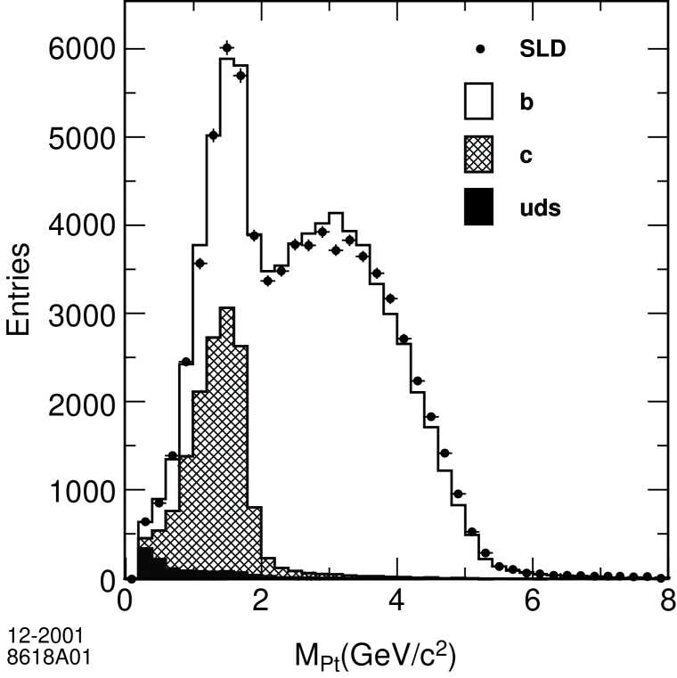
Figure 1: Distribution of the reconstructed $P_{t}$-corrected vertex mass (points). The simulated distribution is also shown (histogram) in which the flavor composition is indicated: $b$ (open), $c$ (cross hatched), and $uds$ (dark shaded).

Figure 1 shows the distribution of $M_{Pt}$ for the selected sample of hemispheres containing a vertex, and the corresponding simulated distribution. $B$-hadron candidates were selected by requiring $M_{Pt}$ $>$ 2.0 GeV/$c^{2}$. We further required $M_{Pt}\leq 2\times M_{ch}$ to reduce the contamination from fake vertices in light-quark events [31]. A total of 42,093 hemispheres were selected, with an estimated efficiency for selecting a true $B$-hemisphere of 43.7%, and a sample purity of 98.2%. The contributions from light-flavors in the sample were 0.34% for primary $u,d$ and $s$ hemispheres and 1.47% for $c$ hemispheres.

3.2 $B$-Hadron Energy Measurement

The energy of each $B$ hadron, $E_{B}$, can be expressed as the sum of the reconstructed-vertex energy, $E_{ch}$, and the energy of those true $B$-decay particles that were missed from the vertex, $E_{0}$. $E_{0}$ can be written

$$E_{0}^{2}=M_{0}^{2}+P_{t}^{2}+P_{0l}^{2}$$ (3)

The two unknowns, $M_{0}$ and $P_{0l}$, must be found in order to obtain $E_{0}$. One kinematic constraint can be obtained by imposing the $B$-hadron mass, $M_{B}$, on the vertex. From Equation (1) we derive the following inequality,

$$\sqrt{M_{ch}^{2}+P_{t}^{2}}+\sqrt{M_{0}^{2}+P_{t}^{2}}\leq M_{B},$$ (4)

where equality holds in the limit that both $P_{0l}$ and $P_{chl}$ vanish in the $B$-hadron rest frame. Equation (4) effectively sets an upper bound on $M_{0}$, $M_{0max}$:

$$M_{0max}^{2}=M_{B}^{2}-2M_{B}\sqrt{M_{ch}^{2}+P_{t}^{2}}+M_{ch}^{2}.$$ (5)

The lower bound is zero. Hence

$$0\leq M_{0}^{2}\leq M_{0max}^{2},$$ (6)

and we expect to obtain a good estimate of $M_{0}$, and therefore of the $B$-hadron energy, when $M_{0max}^{2}$ is small.

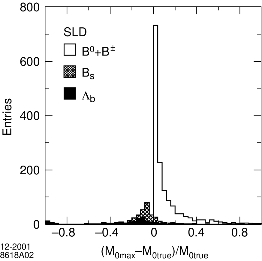
Figure 2: The relative deviation of the maximum missing mass from the true missing mass for simulated $B$ hadron decays; the contributions from different $B$ species are indicated separately: $B^{0}$ and $B^{\pm}$ (open), $B_{s}^{0}$ (cross-hatched), and $\Lambda_{b}$ (dark shaded).

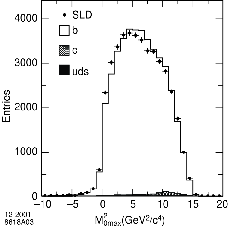
Figure 3: Distribution of the reconstructed $M_{0max}^{2}$ for the selected vertices (points). The simulated distribution is also shown (histogram) in which the flavor composition is indicated: $b$ (open), $c$ (cross hatched), and $uds$ (dark shaded).

We used our simulation to study this issue. We find that the true value of $M_{0}$ tends to cluster near its maximum value $M_{0max}$. Figure 2 shows the relative deviation of $M_{0max}$ from the true $M_{0}$ for all $B$ hadrons, assuming $M_{B}=$ 5.28 GeV/$c^{2}$ in Eq. (5). Although approximately 20% of the $B$ hadrons are $B^{0}_{s}$ and $\Lambda_{b}$, which have larger masses than the $B^{0}$ and $B^{\pm}$, the values of $M_{0max}$ obtained using $M_{B}$=5.28 GeV/$c^{2}$ are typically within about 10% of $M_{0}$. The distribution of the reconstructed $M_{0max}^{2}$ for vertices in the selected-hemisphere sample is shown in Figure 3; the negative tail is an effect of detector resolution. The simulation is in good agreement with the data, and implies that the non-$B$ background is concentrated at high $M_{0max}^{2}$; this is because most of the light-flavor vertices have small $M_{Pt}$ and therefore, due to the strong negative correlation between $M_{Pt}$ and $M_{0max}$, large $M_{0max}$.

Because, for true $B$ decays, $M_{0}$ peaks near $M_{0max}$, we set $M_{0}^{2}$ = $M_{0max}^{2}$ if $M_{0max}^{2}$ $\geq$0, and $M_{0}^{2}$ = 0 if $M_{0max}^{2}$ $<$0. We then calculated $P_{0l}$:

$$P_{0l}=\frac{\textstyle M_{B}^{2}-(M_{ch}^{2}+P_{t}^{2})-(M_{0}^{2}+P_{t}^{2})}{\textstyle 2(M_{ch}^{2}+P_{t}^{2})}P_{chl},$$ (7)

and hence $E_{0}$ (Equation (3)). We divided the reconstructed $B$-hadron energy, $E_{B}^{rec}=E_{0}+E_{ch}$, by the beam energy, $E_{beam}$, to obtain the reconstructed scaled $B$-hadron energy, $x_{B}^{rec}$.

The resolution of $x_{B}^{rec}$ depends on both $M_{0max}^{2}$ and the true $x_{B}$, $x_{B}^{true}$. Using our simulation we found that vertices that have $M_{0max}^{2}<-1.0(GeV/c^{2})^{2}$ are often poorly reconstructed; we rejected them from further analysis. Vertices with small values of $|M_{0max}^{2}|$ are typically reconstructed with better resolution and an upper cut on $M_{0max}^{2}$ was hence applied. For an $x_{B}$-independent $M_{0max}^{2}$ cut we found that the efficiency for selecting $B$ hadrons is roughly linear in $x_{B}$. In order to obtain an approximately $x_{B}$-independent selection efficiency we required:

$$M_{0max}^{2}<\left\{1.1+0.007(E_{beam}-E_{B}^{rec})+4.0exp[-(E_{B}^{rec}-5.5)/3.5]\right\}^{2},$$ (8)

where the two ad hocterms that depend on $E_{B}^{rec}$ increase the efficiency at lower $B$-hadron energy.

In addition, in order to reduce the light-flavor background, each vertex was required to contain at least 3 quality tracks with a normalized impact parameter greater than 2. This cut reduces the dependence of the reconstructed $B$-hadron energy distribution on the light-flavor simulation in the low-energy region.

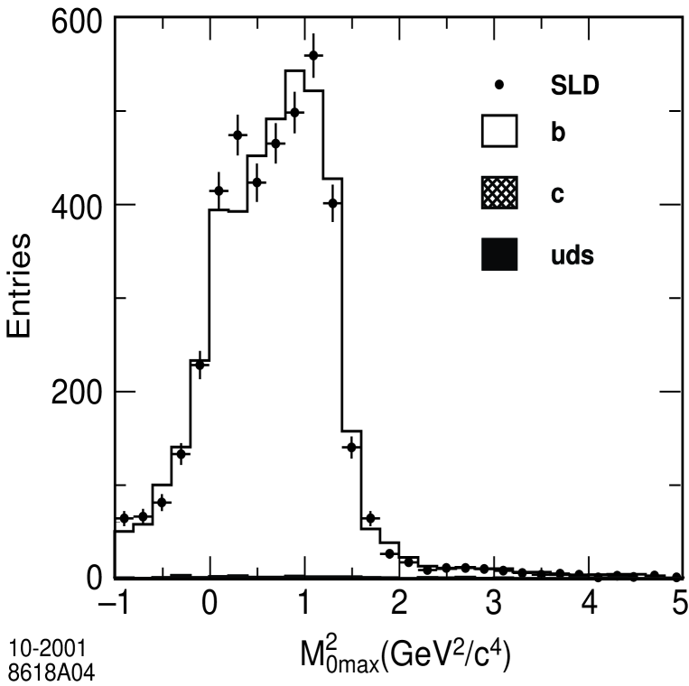
Figure 4: Distribution of the reconstructed $M_{0max}^{2}$ for the final selected sample (see text). The simulated distribution is also shown (histogram) in which the flavor composition is indicated: $b$ (open), $c$ (cross hatched), and $uds$ (dark shaded).

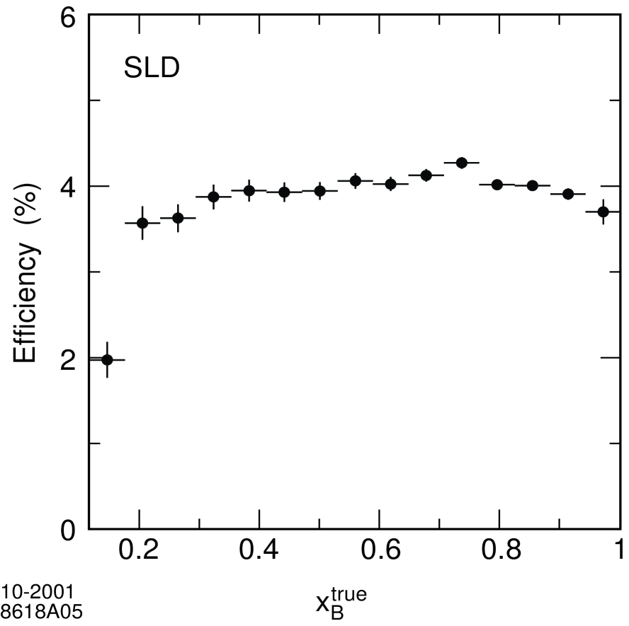
Figure 5: The simulated efficiency for selecting $B$ hadrons as a function of the true scaled $B$-hadron energy, $x_{B}^{true}$.

A total of 4,164 hemispheres contained vertices that satisfied these selection cuts. Figure 4 shows the distribution of $M_{0max}^{2}$; the simulation and data are in good agreement. We calculated that the efficiency for selecting $B$ hadrons is 4.17% and the $B$-hadron purity is 99.0%, with a $uds$ (charm) background of 0.4% (0.6%). The efficiency as a function of the true $x_{B}$ value, $x_{B}^{true}$, is shown in Figure 5. The dependence is weak except for the lowest $x_{B}$ region; the efficiency is substantial, even just above the kinematic threshold.

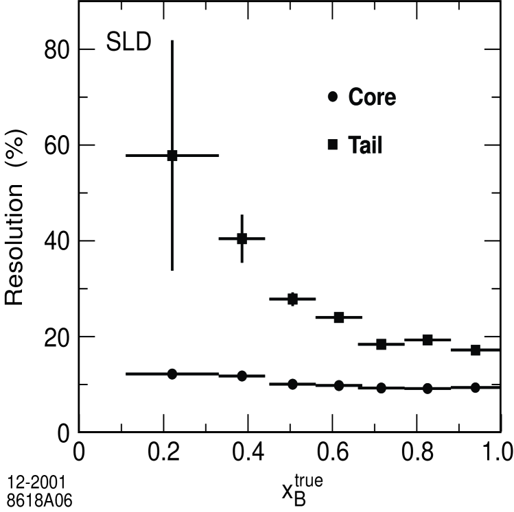
Figure 6: The fitted core and tail widths (see text) of the $B$-energy resolution as a function of the true scaled $B$-hadron energy.

We examined the energy resolution of this technique using simulated events. The distribution of the normalized difference between the true and reconstructed scaled $B$-hadron energies, $(x_{B}^{rec}-x_{B}^{true})/x_{B}^{true}$, was fitted with the sum of two Gaussians. A feature of the analysis is that the distribution is symmetric and the fitted means are consistent with zero. The fit yields a core width (the width of the narrower Gaussian) of 9.6% and a tail width (the width of the wider Gaussian) of 21.2%, with the narrower Gaussian representing a population fraction of 83.6%. Figure 6 shows the core and tail widths as a function of $x_{B}^{true}$, where, in order to compare the widths from different $x_{B}$ bins, the ratio between the core and tail populations was fixed to that obtained above. The $x_{B}$-dependence of the resolution is weak. The resolution is good even at low $B$ energy, which is an advantage of this energy reconstruction technique.

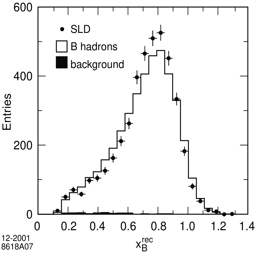
Figure 7: Distribution of the reconstructed scaled $B$-hadron energy (points) and the default Monte Carlo simulation (histogram). The solid histogram shows the simulated non-$B$ background.

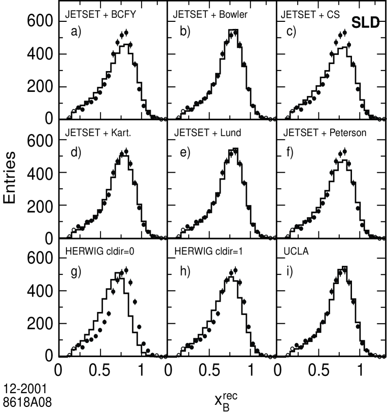
Figure 8: The background-subtracted distribution of reconstructed $B$-hadron energy (points). Also shown (histograms) in (a)-(f) are the predictions of the optimised models within JETSET (see text). (g), (h) show the predictions of HERWIG, and (i) of the UCLA model. Data points excluded from the fit are represented by open circles.

Figure 7 shows the distribution of the reconstructed scaled $B$-hadron energy; the simulated distribution is also shown. The small non-$B$ background, the high $B$ selection efficiency over the full kinematic coverage, and the good energy resolution combine to give a much improved sensitivity of the data to the underlying true shape of the $B$ energy distribution (see next section). The distribution of the non-$B$ background was subtracted bin-by-bin to yield $D^{rec}(x_{B}^{rec})$, which is shown in Fig. 8.

The JETSET event generator used in our simulation is based on a perturbative QCD ‘parton shower’ for production of quarks and gluons, together with the phenomenological Peterson function [9] (Table 1) to account for the fragmentation of $b$ and $c$ quarks into $B$ and $D$ hadrons, respectively, within the iterative Lund string hadronisation mechanism [26]. It is apparent that this simulation does not reproduce the data (Figure 7); the $\chi^{2}$ for the comparison is 70.3 for 16 bins.

4 The Shape of the $B$-Hadron Energy Distribution

4.1 Tests of $b$-Quark Fragmentation Models $f(z,\beta)$

We tested models of $b$-quark fragmentation. Since the resulting fragmentation functions are usually functions of an experimentally-inaccessible variable $z$, eg.$z=(E+p_{\|})_{H}/(E+p_{\|})_{Q}$ or $z={p_{\|}}_{H}/{p_{\|}}_{Q}$, where $p_{\|}$ represents the hadron momentum along the primary heavy-quark momentum vector, it is necessary to use a Monte Carlo generator to produce events according to a given input fragmentation function $f(z,\beta)$, where $\beta$ represents the set of model arbitrary parameters.

We considered the phenomenological models of the Lund group [10], Bowler [8], Peterson et al. [9] and Kartvelishvili et al. [7]. We also considered the perturbative QCD calculations of Braaten et al. (BCFY) [5], and of Collins and Spiller (CS) [3]. Table 1 contains a list of the models. We implemented in turn each fragmentation model in JETSET and generated events without detector simulation. In addition, we tested the UCLA fragmentation model [33] with default parameter settings, as there is no explicit parameter for controlling the $B$-hadron energy. We also tested the HERWIG [34] event generator, and used both possible settings of the parameter switch cldir. cldir=1 forces the heavy hadron to continue in the heavy-quark direction in the hadronisation-cluster decay rest frame, and thereby hardens the fragmentation function. cldir=0 suppresses this feature and yields a softer fragmentation function.

Model	$f(z,\beta)$	Reference
BCFY	$\frac{\textstyle z(1-z)^{2}}{\textstyle[1-(1-r)z]^{6}}[3+{\sum_{i=1}^{4}(-z)^{i}f_{i}(r)}]$	[5]
Bowler	$\frac{\textstyle 1}{\textstyle z^{(1+r_{b}bm_{\perp}^{2})}}(1-z)^{a}$exp$(-bm_{\perp}^{2}/z)$	[8]
CS	$(\frac{\textstyle 1-z}{\textstyle z}+\frac{\textstyle(2-z)\epsilon_{b}}{\textstyle 1-z})(1+z^{2})(1-\frac{\textstyle 1}{\textstyle z}-\frac{\textstyle\epsilon_{b}}{\textstyle 1-z})^{-2}$	[3]
Kartvelishvili	$z^{\alpha_{b}}(1-z)$	[7]
Lund	$\frac{\textstyle 1}{\textstyle z}(1-z)^{a}$exp$(-bm_{\perp}^{2}/z)$	[10]
Peterson	$\frac{\textstyle 1}{\textstyle z}(1-\frac{\textstyle 1}{\textstyle z}-\frac{\textstyle\epsilon_{b}}{\textstyle 1-\textstyle z})^{-2}$	[9]

Table 1: $b$-quark fragmentation models used in comparison with the data. For the BCFY model, $f_{1}(r)~{}=~{}3(3-4r)$, $f_{2}(r)~{}=~{}12-23r+26r^{2}$, $f_{3}(r)~{}=~{}(1-r)(9-11r+12r^{2})$, and $f_{4}(r)~{}=~{}3(1-r)^{2}(1-r+r^{2})$.

In order to make a consistent comparison of each model with the data we adopted the following procedure. For each model starting values of the arbitrary parameters, $\beta$, were assigned and the corresponding fragmentation function $f(z,\beta)$ was used to produce the scaled weakly-decaying $B$-hadron energy distribution, $D^{true}_{model}(x_{B}^{true},\beta)$ before simulation of the detector. The corresponding reconstructed distribution, $D^{rec}_{model}(x_{B}^{rec},\beta)$, was derived from the reconstructed distribution generated with our default model, $D^{rec}_{default}(x_{B}^{rec})$ (Fig. 7), by weighting events at the generator level with the weight factor $D^{true}_{model}(x_{B}^{true},\beta)$/$D^{true}_{default}(x_{B}^{true})$. The resulting reconstructed distribution was then compared with the data distribution, and the $\chi^{2}$ value, defined as

$$\chi^{2}=\sum_{i=1}^{N}\left(\frac{\textstyle N_{i}^{data}-rN_{i}^{MC}}{\textstyle\sigma_{i}}\right)^{2}$$ (9)

was calculated, where $N$ is the number of bins used in the comparison, $N_{i}^{data}$ is the number of entries in bin $i$ in the data distribution, and $N_{i}^{MC}$ is the number of entries in bin $i$ in the simulated distribution. $\sigma_{i}$ is the statistical error on the deviation of the observed number of entries for the data from the expected number of entries in bin $i$, which can be expressed as

$$\sigma_{i}^{2}=\left(\sqrt{rN_{i}^{MC}}\right)^{2}+\left(r\sqrt{N_{i}^{MC}}\right)^{2},$$ (10)

where $\left(\sqrt{rN_{i}^{MC}}\right)^{2}$ is the expected statistical variance on the observed number of entries in bin $i$, assuming the model being tested is correct, and $\left(r\sqrt{N_{i}^{MC}}\right)^{2}$ is the statistical variance on the expected number of entries in bin $i$. Since the $\chi^{2}$-test is not statistically effective for bins with a very small number of entries, the third, the fourth, and the last three bins in Figure 7 were excluded from the comparison.

For each model we varied the values of the parameters $\beta$ and repeated the above procedure. The minimum $\chi^{2}$ was found by scanning through the input parameter space, yielding a set of parameters which give an optimal description of the reconstructed data by the fragmentation model in question. The resulting distributions are shown in Figure 8. Table 2 lists the results of the comparisons.

Model	$\chi^{2}/dof$	Parameters	$\langle x_{B}\rangle$
JETSET + BCFY	105/16	$r=0.085$	0.694
JETSET + Bowler*	17/15	$a=1.4,b=1.2,(r_{b}=1)$	0.709
JETSET + CS	142/16	$\epsilon_{b}=0.003$	0.691
JETSET + Kartvelishvili* et al.	32/16	$\alpha_{b}=10.0$	0.708
JETSET + Lund*	17/15	$a=1.4,b=0.4$	0.712
JETSET + Peterson et al.	70/16	$\epsilon_{b}=0.0055$	0.700
HERWIG cldir=0	1015/17	$-$	0.632
HERWIG cldir=1	149/17	$-$	0.676
UCLA*	27/17	$-$	0.718

Table 2: Results of fragmentation model tests. The minimum $\chi^{2}$, number of degrees of freedom, corresponding parameter values, and the mean value of the corresponding $B$-energy distribution are listed. A * indicates those models used below to unfold the data.

We conclude that with our resolution and our current data sample, we are able to distinguish among these fragmentation models. Within the context of the JETSET fragmentation scheme, the Lund and Bowler models are consistent with the data with $\chi^{2}$ probabilities of 31% and 35%, respectively, the Kartvelishvili model is consistent with the data at the 1% level, while the Peterson, BCFY and CS models are found to be inconsistent with the data. The UCLA model is consistent with the data at a level of 6% $\chi^{2}$ probability. The HERWIG model with cldir=0 is confirmed to be much too soft; using cldir=1 results in a harder distribution and a substantial improvement, but it is still too soft relative to the data.

4.2 Tests of Functional Forms $f(x_{B},\lambda)$

We considered the more general question of what functional forms, $f(x_{B},\lambda)$, can be used as estimates of the true scaled $B$-energy distribution. We considered the functional forms of the BCFY, CS, Kartvelishvili, Lund, and Peterson groups in terms of the variable $x_{B}^{true}$. In addition we considered ad hocgeneralisations of the Peterson function (‘F’), an 8th-order polynomial (‘P8’) and a ‘power’ function. These functions are listed in Table 3. Each function vanishes at $x_{B}=0$ and $x_{B}=1$.

Function	$f(x_{B},\lambda)$	Reference
F	$\frac{\textstyle(1+b(1-x_{B}))}{\textstyle x_{B}}(1-\frac{\textstyle c}{\textstyle x_{B}}-\frac{\textstyle d}{\textstyle 1-x_{B}})^{-2}$	[15]
P8	$x_{B}(1-x_{B})(x_{B}-x_{B}^{0})(1+{\sum_{i=1}^{5}p_{i}x_{B}^{i}})$	(see text)
Power	$x_{B}^{\alpha}(1-x_{B})^{\beta}$	(see text)

Table 3: Additional ad hoc$B$ energy functional forms used in comparison with the data; $x_{B}^{0}$ = $M_{B}/E_{beam}$.

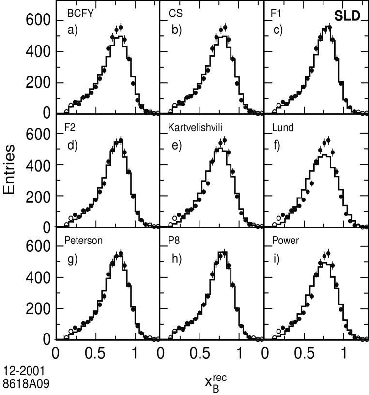
Figure 9: The background-subtracted distribution of reconstructed $B$-hadron energy (points). Also shown (histograms) are the predictions of the optimised functional forms. Data points excluded from the fit are represented by open circles.

For each functional form, a testing procedure similar to that described in subsection 4.1 was applied. The fitted parameters $\lambda$ and the minimum $\chi^{2}$ values are listed in Table 4. The corresponding $D^{rec}_{model}(x_{B}^{rec})$ are compared with the data in Figure 9.

Function	$\chi^{2}/dof$	Parameters	$\langle x_{B}\rangle$
BCFY	73/16	$r=0.248\pm 0.007$	0.704$\pm$0.003
CS	75/16	$\epsilon_{b}=0.0519\pm 0.0036$	0.706$\pm$0.003
Kartvelishvili et al.	138/16	$\alpha_{b}=3.904\pm 0.072$	0.710$\pm$0.003
Lund	252/15	$a=1.88\pm 0.08$	0.715$\pm$0.003
		$bm_{\perp}^{2}=0.32\pm 0.05$
Peterson et al.*	31/16	$\epsilon_{b}=0.0382\pm 0.0016$	0.709$\pm$0.003
F1*	20/15	$c=0.884\pm 0.014$	0.707$\pm$0.003
		$d=0.0181\pm 0.0015$
F2*	31/15	$c=0.976\pm 0.029$	0.710$\pm$0.003
		$d=0.039\pm 0.002$
P8*	12/12	$p_{1}=-9.99\pm 0.25$	0.709$\pm$0.003
		$p_{2}=40.84\pm 0.25$
		$p_{3}=-82.26\pm 0.68$
		$p_{4}=80.90\pm 0.76$
		$p_{5}=-30.60\pm 0.54$
Power	133/15	$\alpha=3.73\pm 0.17$	0.713$\pm$0.003
		$\beta=0.84\pm 0.07$

Table 4: Results of the $\chi^{2}$ fit of ad hocfunctions to the reconstructed scaled $B$-hadron energy distribution. The minimum $\chi^{2}$ value, the number of degrees of freedom, the corresponding parameter values, and the mean value of the corresponding $B$-energy distribution are listed. Errors are statistical only. A * indicates those functions used below to correct the data.

Two sets of optimised parameters were found for the generalised Peterson function F: ‘F1’, obtained by setting the parameter $b$ (Table 3) to infinity, behaves like $x_{B}$ as $x_{B}$ $\rightarrow$0 and $(1-x_{B})^{3}$ as $x_{B}$ $\rightarrow$1 and yields a $\chi^{2}$ probability of 18%; ‘F2’, obtained by setting $b$ to zero, has a $\chi^{2}$ probability of 1.0%. A constrained polynomial of at least 8th-order was needed to obtain a $\chi^{2}$ probability greater than 0.1%. The Peterson function reproduces the data with a $\chi^{2}$ probability of about 1%. The remaining functional forms are found to be inconsistent with the data. The widths of the BCFY and CS functions are too large to describe the data; the Kartvelishvili, Lund and ‘power’ functions vanish too fast as $x_{B}$ $\rightarrow$0. We conclude that, within our resolution and with our current data sample, we are able to distinguish among these ad hocfunctional forms.

5 Correction of the $B$-Energy Distribution

In order to compare our results with those from other experiments and potential future theoretical predictions it is necessary to correct $D^{rec}(x_{B}^{rec})$ for the effects of detector acceptance, event selection and analysis bias, as well as for bin-to-bin migrations caused by the finite resolution of the detector and the analysis technique. Due to the known rapid variation of the a prioriunknown true $B$-energy distribution at large $x_{B}$, any correction procedure will necessarily be model-dependent. We chose a method that allows explicit evaluation of this model-dependence and which gives a very good estimate of the true energy distribution using all of the above models or functional forms that are consistent with the data.

We applied a $25\times 25$ matrix unfolding procedure to $D^{rec}(x_{B}^{rec})$ to obtain an estimate of the true distribution $D^{true}(x_{B}^{true})$, where $x_{B}^{true}$ refers to the weakly-decaying $B$ hadron:

$$D^{true}(x_{B}^{true})\quad=\quad\epsilon^{-1}(x_{B}^{true})\cdot E(x_{B}^{true},x_{B}^{rec})\cdot D^{rec}(x_{B}^{rec})\vspace{-0.5cm}$$ (11)

where $E$ is a matrix to correct for bin-to-bin migrations, and $\epsilon$ is a vector representing the efficiency for selecting true $B$-hadron decays. $E$ and $\epsilon$ were calculated from our MC simulation; the matrix $E$ incorporates a convolution of the input fragmentation function with the resolution of the detector. $E(i,j)$ is the number of vertices with $x_{B}^{true}$ in bin $i$ and $x_{B}^{rec}$ in bin $j$, normalized by the total number of vertices with $x_{B}^{rec}$ in bin $j$.

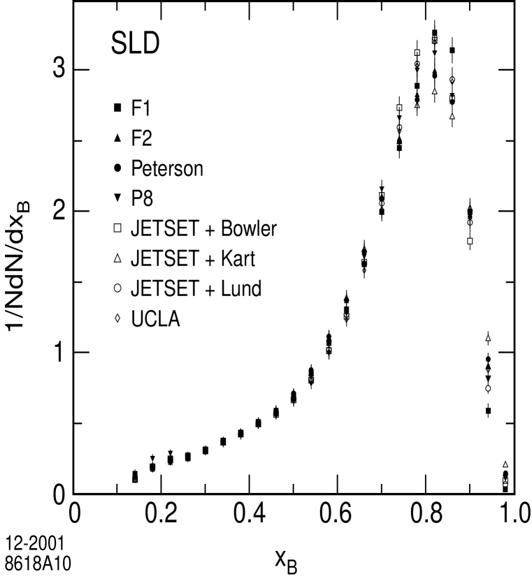
Figure 10: Distributions of the scaled weakly-decaying $B$-hadron energy unfolded using different input models or functions (see text).

We evaluated $E$ by using in turn the Monte Carlo simulation weighted according to each input generator-level true $B$ energy distribution found to be consistent with the data in Section 4. We considered in turn each of the eight consistent distributions, using the optimised parameters listed in Tables 2 and 4. The matrix $E$ was then evaluated by examining the population migrations of true $B$ hadrons between bins of the input scaled $B$ energy, $x_{B}^{true}$, and the reconstructed scaled $B$ energy, $x_{B}^{rec}$. Using each $D^{true}_{model}(x_{B}^{true})$, the data distribution $D^{rec}(x_{B}^{rec})$ was then unfolded according to Equation (11) to yield $D^{true}(x_{B}^{true})$, which is shown for each input fragmentation function in Figure 10. It can be seen that the shapes of $D^{true}(x_{B}^{true})$ differ systematically among the input scaled $B$-energy distributions. These differences were used to assign systematic errors.

6 Systematic Errors

We considered sources of systematic uncertainty that potentially affect our measurement. These may be divided into uncertainties in modelling the detector and uncertainties on experimental measurements serving as input parameters to the underlying physics modelling. For each source of systematic error, the Monte Carlo distribution $D^{true}_{default}(x_{B}^{true})$ was re-weighted and then the resulting new reconstructed distribution, $D^{rec}_{new}(x_{B}^{rec})$, was compared with the data $D^{rec}(x_{B}^{rec})$ by repeating the fitting and unfolding procedures described in Sections 4 and 5. The differences in both the shape and the mean value of the $x_{B}^{true}$ distribution relative to the default procedure were considered.

Ad hoc corrections were applied to the simulations of four track-related quantities to account for discrepancies w.r.t. the data, namely the tracking efficiency and the distributions of track $p_{\perp}$, polar angle and the projection of the impact parameter along the $z$ axis. In each case a systematic error was assigned (see Table 5) using half the difference between the results obtained with the default and corrected simulations.

A large number of measured quantities relating to the production and decay of charm and bottom hadrons are used as input to our simulation. In $b\bar{b}$events we considered the uncertainties on: the branching fraction for $Z^{0}$ $\rightarrow$$b\bar{b}$; the rates of production of $B^{\pm}$, $B^{0}$ and $B^{0}_{s}$ mesons, and $b$ baryons; the lifetimes of $B$ mesons and baryons; and the average $B$ hadron decay charged multiplicity. In $c\bar{c}$events we considered the uncertainties on: the branching fraction for $Z^{0}$ $\rightarrow$$c\bar{c}$, the charmed hadron lifetimes, the charged multiplicity of charmed hadron decays, the production of $K^{0}$ from charmed hadron decays, and the fraction of charmed hadron decays containing no $\pi^{0}$s. We also considered the rate of production of $s\bar{s}$ in the jet fragmentation process, and the production of secondary $b\bar{b}$and $c\bar{c}$from gluon splitting. The world-average values and their respective uncertainties [12, 32] were used in our simulation and are listed in Table 5. Most of these variations affect the normalisation, but have very little effect on the shape or the mean value. In no case do we find a variation that changes our conclusion about which models and functions are consistent with the data. The systematic errors on the mean value are listed in Table 5.

Source	Variation	$\delta$ $\langle x_{B}\rangle$
Tracking efficiency correction	-1.5$\pm$0.75%	0.0007
Impact parameter smearing in $z$	9.0$\pm$4.5$\mu$m	0.0006
Track polar angle smearing	1.0$\pm$0.5 mrad	0.0002
Track $1/p_{\perp}$ smearing	0.8$\pm$0.4 MeV-1	0.0013
Detector total		0.0016
$B^{+}$ production fraction	0.39$\pm$0.11	$\mp$0.0001
$B^{0}$ production fraction	0.39$\pm$0.11	$<$0.0001
$B_{s}$ production fraction	0.098$\pm$0.0012	$\pm$0.0003
$\Lambda_{b}$ production fraction	0.103$\pm$0.018	$<$0.0001
$B\!\rightarrow$ charm multiplicity and species	[19]	$\pm$0.0006
$B\!\rightarrow K^{0}$ multiplicity	0.658$\pm$0.066	$\pm$0.0009
$B\!\rightarrow\Lambda^{0}$ multiplicity	0.124$\pm$0.008	$\pm$0.0002
$B$ decay $<n_{ch}>$	4.955$\pm$0.062	${}^{-0.0004}_{+0.0001}$
$D\rightarrow K^{0}$ multiplicity	[19]	$\pm 0.0014$
$D\rightarrow$ no $\pi^{0}$ fraction	[19]	$\pm$0.0006
$D$ decay $<n_{ch}>$	[19]	$\pm$0.0003
$g\rightarrow b\bar{b}$	0.00254$\pm$0.00050 /evt	$\pm$0.0001
$g\rightarrow c\bar{c}$	0.0299$\pm$0.0039 /evt	$\pm$0.0003
$B^{0}$ mass	5.2794$\pm$ 0.0005 GeV/$c^{2}$	$<$0.0001
$b$, $c$ hadron lifetimes, $R_{b}$, $R_{c}$	[35]	$\pm$0.0002
Physics total		0.0020
Monte Carlo statistics		0.0008
Total systematic		0.0027

Table 5: Uncertainty source, range of variation and size of the resulting systematic error on $<x_{B}>$.

Other relevant systematic effects such as variation of the event selection cuts and the assumed $B$-hadron mass were also found to be very small. As a cross-check, we varied the $M_{0max}$ cut (Equation (8)) used to select the final $B$ sample and repeated the analysis procedure. In each case, conclusions about the shape of the $B$ energy distribution hold. In each bin, all sources of systematic uncertainty were added in quadrature to obtain the total systematic error.

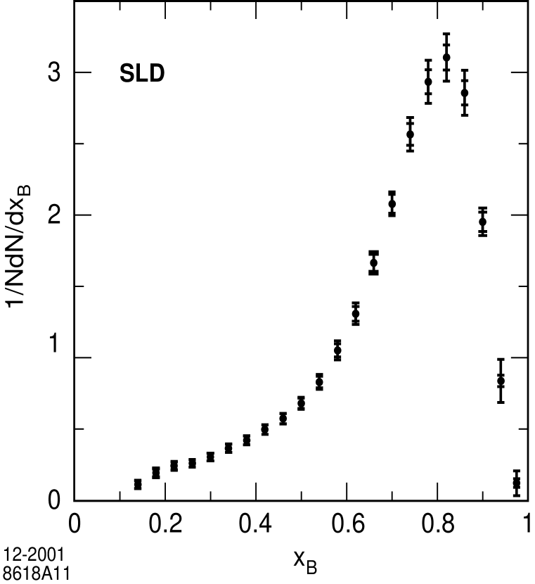
Figure 11: Final distribution of the weakly-decaying scaled $B$-hadron energy. In each bin the central value is the average of the eight distributions shown in Fig. 10, the inner error bar represents the experimental error, and the outer error bar represents the sum in quadrature of the experimental and unfolding errors.

The model-dependence of the unfolding procedure was estimated by considering the envelope of the unfolded results shown in Figure 10. Since eight models or functions are consistent with the data, in each bin of $x_{B}^{true}$ we calculated the average value of these eight unfolded results as well as the r.m.s. deviation; the average was taken as our central value and the deviation was assigned as the unfolding uncertainty. Figure 11 shows the final corrected $x_{B}$ distribution $D(x_{B})$. The data are listed in Table 6 Since two of the eight functions (the Kartvelishvili model and the Peterson functional form) are only in marginal agreement with the data, and the 8th-order polynomial has an unphysical behavior near $x_{B}=1$, this r.m.s. may be considered to be a rather reasonable envelope within which the true $x_{B}$ distribution is most likely to vary. The model dependence of this analysis is significantly smaller than that of previous direct $B$-energy measurements, indicating the enhanced sensitivity of our data to the underlying true energy distribution.

$x_{B}$ range	$D(x_{B})$	stat.	systematic	unfolding	total
$0.00<x_{B}<0.04$	0.000	0.000	0.000	0.000	0.000
$0.04<x_{B}<0.08$	0.000	0.000	0.000	0.000	0.000
$0.08<x_{B}<0.12$	0.000	0.000	0.000	0.000	0.000
$0.12<x_{B}<0.16$	0.110	0.029	0.004	0.014	0.034
$0.16<x_{B}<0.20$	0.188	0.035	0.005	0.025	0.043
$0.20<x_{B}<0.24$	0.204	0.032	0.006	0.013	0.036
$0.24<x_{B}<0.28$	0.213	0.027	0.008	0.010	0.030
$0.28<x_{B}<0.32$	0.268	0.031	0.009	0.015	0.036
$0.32<x_{B}<0.36$	0.340	0.036	0.011	0.011	0.039
$0.36<x_{B}<0.40$	0.398	0.037	0.012	0.010	0.041
$0.40<x_{B}<0.44$	0.505	0.041	0.014	0.016	0.045
$0.44<x_{B}<0.48$	0.587	0.042	0.015	0.015	0.048
$0.48<x_{B}<0.52$	0.677	0.044	0.016	0.011	0.050
$0.52<x_{B}<0.56$	0.796	0.047	0.017	0.030	0.059
$0.56<x_{B}<0.60$	0.991	0.052	0.018	0.056	0.079
$0.60<x_{B}<0.64$	1.241	0.058	0.018	0.070	0.092
$0.64<x_{B}<0.68$	1.622	0.068	0.020	0.062	0.093
$0.68<x_{B}<0.72$	2.092	0.080	0.028	0.044	0.096
$0.72<x_{B}<0.76$	2.671	0.094	0.046	0.075	0.128
$0.76<x_{B}<0.80$	3.102	0.104	0.071	0.140	0.189
$0.80<x_{B}<0.84$	3.290	0.111	0.084	0.201	0.245
$0.84<x_{B}<0.88$	2.953	0.106	0.065	0.144	0.190
$0.88<x_{B}<0.92$	1.897	0.079	0.094	0.113	0.167
$0.92<x_{B}<0.96$	0.753	0.042	0.051	0.205	0.215
$0.96<x_{B}<1.00$	0.090	0.011	0.004	0.061	0.063

Table 6: The scaled $B$-hadron energy distribution.

The statistical correlation matrix is shown in Table 7.

Bin	4	5	6	7	8	9	10	11	12	13	14	15	16	17	18	19	20	21	22	23	24	25
5	69.4
6	42.0	79.0
7	19.3	46.5	80.7
8	7.1	23.5	47.2	82.3
9	6.9	10.6	18.3	39.6	79.0
10	4.8	6.0	9.8	20.9	48.5	82.1
11	3.3	0.5	2.4	7.6	20.1	46.9	83.1
12	5.6	1.1	1.5	2.6	7.1	23.1	54.0	87.7
13	5.8	0.1	-2.2	-2.5	-1.4	4.4	19.6	51.2	82.2
14	-0.3	-1.8	-2.8	-3.2	-2.9	-0.1	7.8	28.4	53.8	86.0
15	-4.5	-4.6	-6.7	-6.8	-7.6	-7.5	-4.6	7.6	24.2	55.6	86.3
16	-7.2	-9.8	-12.6	-13.3	-13.7	-12.8	-13.3	-7.6	1.4	24.6	56.5	88.6
17	-7.8	-11.5	-13.9	-15.4	-18.1	-19.2	-21.1	-19.1	-15.5	-3.1	18.4	55.4	85.8
18	-7.7	-15.0	-19.8	-22.6	-25.1	-26.1	-28.8	-29.1	-29.5	-24.8	-14.8	12.8	47.2	82.6
19	-12.0	-19.5	-24.0	-28.1	-31.8	-33.4	-36.4	-38.0	-40.1	-39.5	-38.4	-24.4	1.3	39.1	80.6
20	-12.2	-22.9	-29.2	-33.9	-37.5	-38.8	-43.4	-48.2	-53.0	-55.3	-57.9	-50.8	-33.6	-5.3	37.5	80.3
21	-15.3	-22.3	-27.3	-30.8	-33.8	-35.7	-40.3	-44.2	-47.4	-50.1	-57.7	-64.0	-62.5	-51.3	-19.8	28.7	77.8
22	-13.9	-18.6	-22.7	-25.9	-28.8	-30.5	-34.5	-38.4	-42.0	-45.5	-52.0	-58.5	-60.7	-59.5	-45.2	-12.1	39.2	85.6
23	-10.5	-13.1	-16.3	-18.8	-21.1	-22.3	-24.7	-27.8	-30.7	-33.9	-39.7	-46.3	-50.7	-54.6	-52.2	-36.9	0.8	52.1	85.8
24	-7.4	-9.3	-11.4	-13.0	-14.5	-15.5	-17.4	-19.8	-21.5	-23.8	-28.3	-33.5	-37.5	-41.7	-43.3	-38.1	-15.8	23.9	57.7	89.1
25	-5.1	-6.4	-7.7	-8.1	-9.0	-10.3	-11.8	-13.7	-14.7	-16.0	-19.2	-22.9	-25.8	-28.7	-30.9	-30.3	-19.0	6.2	32.9	68.8	91.2

Table 7: The statistical correlation matrix (%).

7 Summary and Conclusions

We have used the excellent tracking and vertexing capabilities of SLD to reconstruct the energies of $B$ hadrons in $e^{+}e^{-}$$\rightarrow$$Z^{0}$ events over the full kinematic range by applying a new kinematic technique to an inclusive sample of reconstructed $B$-hadron decay vertices. The $B$ selection efficiency of the method is 4.2% and the resolution on the $B$ energy is about 9.6% for roughly 83% of the reconstructed decays. The energy resolution for low-energy $B$ hadrons is significantly better than in previous measurements.

We compared our measurement with several models of $b$-quark fragmentation. The Bowler, Lund and Kartvelishivili et al.models, implemented within the JETSET string fragmentation scheme, describe our data, as does the UCLA model. None of the Braaten et al., Collins-Spiller or Peterson et al.models implemented within JETSET, nor HERWIG, describes the data.

The raw scaled $B$-energy distribution was corrected for bin-to-bin migrations caused by the resolution of the method, and for selection efficiency, to derive an estimate of the underlying true distribution for weakly-decaying $B$ hadrons produced in $Z^{0}$ decays. Systematic uncertainties in the correction were evaluated and found to be significantly smaller than those of previous direct $B$-energy measurements. The final corrected $x_{B}$ distribution $D(x_{B})$ is shown in Figure 11. This result is consistent with, and supersedes, our previous measurements [17, 18]. It is also consistent with a recent precise measurement [36]

It is conventional to evaluate the mean of this $B$-energy distribution, $<x_{B}>$. For each of the seven parameter-dependent functions that provide a reasonable description of the data we evaluated $<x_{B}>$ from the distribution that corresponds to the optimised parameter(s); these are listed in Table 2 and Table 4. For the UCLA model, which contains no arbitrary parameters relating to $b$-quark fragmentation, we evaluated $<x_{B}>$ from the corresponding unfolded distribution shown in Fig. 10; this yields $<x_{B}>$ = 0.712. We took the average of the eight values of $<x_{B}>$ as our central value, and defined the model-dependent uncertainty to be the r.m.s. deviation. We obtained

$$<x_{B}>\quad=\quad 0.709\pm 0.003(stat.)\pm 0.003(syst.)\pm 0.002(model),$$ (12)

It can be seen that $<x_{B}>$ is relatively insensitive to the variety of allowed forms of the shape of the fragmentation function.

^∗∗List of Authors

Koya Abe,⁽²⁴⁾ Kenji Abe,⁽¹⁵⁾ T. Abe,⁽²¹⁾ I. Adam,⁽²¹⁾ H. Akimoto,⁽²¹⁾ D. Aston,⁽²¹⁾ K.G. Baird,⁽¹¹⁾ C. Baltay,⁽³⁰⁾ H.R. Band,⁽²⁹⁾ T.L. Barklow,⁽²¹⁾ J.M. Bauer,⁽¹²⁾ G. Bellodi,⁽¹⁷⁾ R. Berger,⁽²¹⁾ G. Blaylock,⁽¹¹⁾ J.R. Bogart,⁽²¹⁾ G.R. Bower,⁽²¹⁾ J.E. Brau,⁽¹⁶⁾ M. Breidenbach,⁽²¹⁾ W.M. Bugg,⁽²³⁾ D. Burke,⁽²¹⁾ T.H. Burnett,⁽²⁸⁾ P.N. Burrows,⁽¹⁷⁾ A. Calcaterra,⁽⁸⁾ R. Cassell,⁽²¹⁾ A. Chou,⁽²¹⁾ H.O. Cohn,⁽²³⁾ J.A. Coller,⁽⁴⁾ M.R. Convery,⁽²¹⁾ V. Cook,⁽²⁸⁾ R.F. Cowan,⁽¹³⁾ G. Crawford,⁽²¹⁾ C.J.S. Damerell,⁽¹⁹⁾ M. Daoudi,⁽²¹⁾ N. de Groot,⁽²⁾ R. de Sangro,⁽⁸⁾ D.N. Dong,⁽¹³⁾ M. Doser,⁽²¹⁾ R. Dubois, I. Erofeeva,⁽¹⁴⁾ V. Eschenburg,⁽¹²⁾ E. Etzion,⁽²⁹⁾ S. Fahey,⁽⁵⁾ D. Falciai,⁽⁸⁾ J.P. Fernandez,⁽²⁶⁾ K. Flood,⁽¹¹⁾ R. Frey,⁽¹⁶⁾ E.L. Hart,⁽²³⁾ K. Hasuko,⁽²⁴⁾ S.S. Hertzbach,⁽¹¹⁾ M.E. Huffer,⁽²¹⁾ X. Huynh,⁽²¹⁾ M. Iwasaki,⁽¹⁶⁾ D.J. Jackson,⁽¹⁹⁾ P. Jacques,⁽²⁰⁾ J.A. Jaros,⁽²¹⁾ Z.Y. Jiang,⁽²¹⁾ A.S. Johnson,⁽²¹⁾ J.R. Johnson,⁽²⁹⁾ R. Kajikawa,⁽¹⁵⁾ M. Kalelkar,⁽²⁰⁾ H.J. Kang,⁽²⁰⁾ R.R. Kofler,⁽¹¹⁾ R.S. Kroeger,⁽¹²⁾ M. Langston,⁽¹⁶⁾ D.W.G. Leith,⁽²¹⁾ V. Lia,⁽¹³⁾ C. Lin,⁽¹¹⁾ G. Mancinelli,⁽²⁰⁾ S. Manly,⁽³⁰⁾ G. Mantovani,⁽¹⁸⁾ T.W. Markiewicz,⁽²¹⁾ T. Maruyama,⁽²¹⁾ A.K. McKemey,⁽³⁾ R. Messner,⁽²¹⁾ K.C. Moffeit,⁽²¹⁾ T.B. Moore,⁽³⁰⁾ M. Morii,⁽²¹⁾ D. Muller,⁽²¹⁾ V. Murzin,⁽¹⁴⁾ S. Narita,⁽²⁴⁾ U. Nauenberg,⁽⁵⁾ H. Neal,⁽³⁰⁾ G. Nesom,⁽¹⁷⁾ N. Oishi,⁽¹⁵⁾ D. Onoprienko,⁽²³⁾ L.S. Osborne,⁽¹³⁾ R.S. Panvini,⁽²⁷⁾ C.H. Park,⁽²²⁾ I. Peruzzi,⁽⁸⁾ M. Piccolo,⁽⁸⁾ L. Piemontese,⁽⁷⁾ R.J. Plano,⁽²⁰⁾ R. Prepost,⁽²⁹⁾ C.Y. Prescott,⁽²¹⁾ B.N. Ratcliff,⁽²¹⁾ J. Reidy,⁽¹²⁾ P.L. Reinertsen,⁽²⁶⁾ L.S. Rochester,⁽²¹⁾ P.C. Rowson,⁽²¹⁾ J.J. Russell,⁽²¹⁾ O.H. Saxton,⁽²¹⁾ T. Schalk,⁽²⁶⁾ B.A. Schumm,⁽²⁶⁾ J. Schwiening,⁽²¹⁾ V.V. Serbo,⁽²¹⁾ G. Shapiro,⁽¹⁰⁾ N.B. Sinev,⁽¹⁶⁾ J.A. Snyder,⁽³⁰⁾ H. Staengle,⁽⁶⁾ A. Stahl,⁽²¹⁾ P. Stamer,⁽²⁰⁾ H. Steiner,⁽¹⁰⁾ D. Su,⁽²¹⁾ F. Suekane,⁽²⁴⁾ A. Sugiyama,⁽¹⁵⁾ A. Suzuki,⁽¹⁵⁾ M. Swartz,⁽⁹⁾ F.E. Taylor,⁽¹³⁾ J. Thom,⁽²¹⁾ E. Torrence,⁽¹³⁾ T. Usher,⁽²¹⁾ J. Va’vra,⁽²¹⁾ R. Verdier,⁽¹³⁾ D.L. Wagner,⁽⁵⁾ A.P. Waite,⁽²¹⁾ S. Walston,⁽¹⁶⁾ A.W. Weidemann,⁽²³⁾ E.R. Weiss,⁽²⁸⁾ J.S. Whitaker,⁽⁴⁾ S.H. Williams,⁽²¹⁾ S. Willocq,⁽¹¹⁾ R.J. Wilson,⁽⁶⁾ W.J. Wisniewski,⁽²¹⁾ J.L. Wittlin,⁽¹¹⁾ M. Woods,⁽²¹⁾ T.R. Wright,⁽²⁹⁾ R.K. Yamamoto,⁽¹³⁾ J. Yashima,⁽²⁴⁾ S.J. Yellin,⁽²⁵⁾ C.C. Young,⁽²¹⁾ H. Yuta.⁽¹⁾

⁽¹⁾Aomori University, Aomori, 030 Japan, ⁽²⁾University of Bristol, Bristol, United Kingdom, ⁽³⁾Brunel University, Uxbridge, Middlesex, UB8 3PH United Kingdom, ⁽⁴⁾Boston University, Boston, Massachusetts 02215, ⁽⁵⁾University of Colorado, Boulder, Colorado 80309, ⁽⁶⁾Colorado State University, Ft. Collins, Colorado 80523, ⁽⁷⁾INFN Sezione di Ferrara and Universita di Ferrara, I-44100 Ferrara, Italy, ⁽⁸⁾INFN Laboratori Nazionali di Frascati, I-00044 Frascati, Italy, ⁽⁹⁾Johns Hopkins University, Baltimore, Maryland 21218-2686, ⁽¹⁰⁾Lawrence Berkeley Laboratory, University of California, Berkeley, California 94720, ⁽¹¹⁾University of Massachusetts, Amherst, Massachusetts 01003, ⁽¹²⁾University of Mississippi, University, Mississippi 38677, ⁽¹³⁾Massachusetts Institute of Technology, Cambridge, Massachusetts 02139, ⁽¹⁴⁾Institute of Nuclear Physics, Moscow State University, 119899 Moscow, Russia, ⁽¹⁵⁾Nagoya University, Chikusa-ku, Nagoya, 464 Japan, ⁽¹⁶⁾University of Oregon, Eugene, Oregon 97403, ⁽¹⁷⁾Oxford University, Oxford, OX1 3RH, United Kingdom, ⁽¹⁸⁾INFN Sezione di Perugia and Universita di Perugia, I-06100 Perugia, Italy, ⁽¹⁹⁾Rutherford Appleton Laboratory, Chilton, Didcot, Oxon OX11 0QX United Kingdom, ⁽²⁰⁾Rutgers University, Piscataway, New Jersey 08855, ⁽²¹⁾Stanford Linear Accelerator Center, Stanford University, Stanford, California 94309, ⁽²²⁾Soongsil University, Seoul, Korea 156-743, ⁽²³⁾University of Tennessee, Knoxville, Tennessee 37996, ⁽²⁴⁾Tohoku University, Sendai, 980 Japan, ⁽²⁵⁾University of California at Santa Barbara, Santa Barbara, California 93106, ⁽²⁶⁾University of California at Santa Cruz, Santa Cruz, California 95064, ⁽²⁷⁾Vanderbilt University, Nashville,Tennessee 37235, ⁽²⁸⁾University of Washington, Seattle, Washington 98105, ⁽²⁹⁾University of Wisconsin, Madison,Wisconsin 53706, ⁽³⁰⁾Yale University, New Haven, Connecticut 06511.

References

- [1]
- [2] See e.g. J.D. Bjorken, Phys. Rev.D17 (1978) 171.
- [3] P.D.B. Collins and T.P. Spiller, J. Phys. G 11 (1985) 1289.
-
[4]
B. Mele and P. Nason, Phys. Lett. B245 (1990) 635.
B. Mele and P. Nason, Nucl. Phys. B361 (1991) 626.
G. Colangelo and P. Nason, Phys. Lett. B285 (1992) 167. -
[5]
E. Braaten, K. Cheung, T.C. Yuan, Phys. Rev. D48
(1993) R5049.
E. Braaten, K. Cheung, S. Fleming, T.C. Yuan, Phys. Rev. D51 (1995) 4819. - [6] Yu. L. Dokshitzer, V.A. Khoze, S.I. Troyan, Phys. Rev.D53 (1996) 89.
- [7] V. G. Kartvelishvili, A. K. Likhoded and V. A. Petrov, Phys. Lett. 78B (1978) 615.
- [8] M.G. Bowler, Z. Phys. C11 (1981) 169.
- [9] C. Peterson, D. Schlatter, I. Schmitt and P.M. Zerwas, Phys. Rev. D27 (1983) 105.
- [10] B. Andersson, G. Gustafson, G. Ingelman, T. Sjöstrand, Phys. Rep. 97 (1983) 32.
-
[11]
R.L. Jaffe, L. Randall, Nucl. Phys. B412 (1994) 79.
L. Randall, N. Rius, Nucl. Phys.B441 (1995) 167. - [12] The LEP Electroweak Working Group, D. Abbaneo et al., LEPHF/96-01 (July 1996).
-
[13]
ALEPH Collab., D. Buskulic et al., Z. Phys. C62
(1994) 179.
DELPHI Collab., P. Abreu et al., Z. Phys.C66 (1995) 323.
L3 Collab., O. Adeva et al., Phys Lett. B261 (1991) 177.
OPAL Collab., P.D. Acton et al., Z. Phys. C60 (1993) 199. - [14] See e.g. D.H. Saxon in ‘High Energy Electron-Positron Physics’, Eds. A. Ali, P. Söding, World Scientific 1988, p. 539.
- [15] ALEPH Collab., D. Buskulic et al., Phys. Lett. B357 (1995) 699.
- [16] OPAL Collab., G. Alexander et al., Phys. Lett.B364 (1995) 93.
- [17] SLD Collab., K. Abe et al., Phys. Rev.D56 (1997) 5310.
- [18] SLD Collab., Kenji. Abe et al., Phys. Rev. Lett.84 (2000) 4300.
- [19] D. Dong, Ph. D. thesis, Massachusetts Institute of Technology, SLAC-Report-550 (1999).
- [20] SLD Design Report, SLAC Report 273 (1984).
- [21] SLD Collaboration, K. Abe et al., Phys. Rev. D51 (1995) 962.
- [22] M.D. Hildreth et al., IEEE Trans. Nucl. Sci. 42 (1994) 451.
- [23] K. Abe et al., Nucl. Instr. Meth. A400 (1997) 287.
-
[24]
S. Brandt et al., Phys. Lett. 12 (1964) 57.
E. Farhi, Phys. Rev. Lett. 39 (1977) 1587. - [25] D. Axen et al., Nucl. Inst. Meth. A328 (1993) 472.
- [26] T. Sjöstrand, Comput. Phys. Commun. 82 (1994) 74.
-
[27]
P. N. Burrows, Z. Phys. C41 (1988) 375.
OPAL Collab., M.Z. Akrawy et al., Z. Phys. C47 (1990) 505. - [28] SLD Collab., K. Abe et al., Phys. Rev. Lett. 79 (1997) 590.
- [29] R. Brun et al., Report No. CERN-DD/EE/84-1 (1989).
- [30] D. J. Jackson, Nucl. Inst. and Meth. A388 247 (1997).
- [31] SLD Collab., K. Abe et al., Phys. Rev. Lett. 80 (1998) 660.
- [32] SLD Collab., K. Abe et al., Phys. Rev. D53 (1996) 1023.
- [33] S. Chun and C. Buchanan, Phys. Rep. 292 (1998) 239.
- [34] G. Marchesini et al., Comp. Phys. Comm. 67 (1992) 465.
- [35] ALEPH, CDF, DELPHI, L3, OPAL, SLD Collabs., CERN-EP/2001-050 (2001).
- [36] ALEPH Collab., A Heister et al., Phys. Lett.B512 (2001) 30.