1

A Search for GMSB Sleptons with Lifetime at ALEPH
Luke Timothy Jones
Department of Physics,
Royal Holloway,
University of London.
A thesis submitted to the University of London
for the degree of Doctor of Philosophy.
September, 2001.

Abstract

A search for slepton production via the decay of pair-produced neutralinos has been performed under the assumption that the sleptons have observable lifetime in the detector before each decays to a lepton and a gravitino. Sleptons, neutralinos and gravitinos are particles predicted by the theory of supersymmetry, and are the supersymmetric partners of the Standard Model leptons, neutral bosons and of the graviton respectively. The search was performed in 628 $\mathrm{pb}$^-1 of data taken by the ALEPH detector at LEP centre-of-mass energies from 189 to 208 $\mathrm{GeV}$. It was motivated by general predictions of Gauge-Mediated Supersymmetry Breaking (GMSB) models in which the lightest supersymmetric particle is always the gravitino. No evidence of the process was found. Model-independent cross-section limits are quoted as a function of neutralino mass, slepton mass and slepton lifetime in the case that the neutralino branching ratios to each slepton are equal at $\frac{1}{3}$ (the so-called slepton co-NLSP scenario, where NLSP stands for ‘Next-to-Lightest Supersymmetric Particle’) and in the case that the neutralino decays exclusively to the stau (the stau-NLSP scenario). Excluded regions in the neutralino-stau mass plane are shown for four gravitino masses under model-specific assumptions.

Acknowledgements

I would like to thank…
$\cdot$ Grahame Blair and Terry Medcalf for being my supervisors. $\cdot$ Jon Chambers and Julian Von Wimmersburg for holding my hand during my first tottering steps into the worlds of Unix, Hbook and Paw. $\cdot$ Jeremy Coles, Nick Robertson, John Kennedy, David Smith and all the other friends I made at CERN for advice, support and friendship, sorry I can’t name you all – you know who you are! $\cdot$ Clemens Mannert for kindly providing me with the modified versions of GALEPH and other packages that were absolutely necessary for my search and which would have taken me months to do myself, plus the plain-English documentation of how to use them. $\cdot$ Simon George and all the technical support staff in the group, without whom our computers would be expensive paperweights. $\cdot$ Glen Cowan for help on all matters statistical. $\cdot$ Aran Garcia-Bellido, especially for his patience and assistance while I debugged the exclusion routine. $\cdot$ Grahame Blair (again), Mike Green and Glen Cowan (again) for reading my thesis and giving me invaluable feedback. $\cdot$ Anybody who has lent me, or offered to lend me, money during the financial wilderness of this last year (especially my parents), or anyone who lent me a TV (I suppose that’s just you then Bodger). $\cdot$ I would also like to thank every single one of the friends I have known over the past four years by name, all of whom have provided much needed (and frequently pub-oriented) distractions from particle physics and life as a Royal Holloway student, but I’d inevitably forget some people so I’ll just say – if you’ve been a mate, thanks.

Declaration

The copyright of this thesis rests with the author and no quotation from it or information derived from it may be published without the prior written consent of the author.
                                                                                       Luke Jones.

Chapter 1 Introduction

This thesis documents a search for evidence of supersymmetry, which is a theory relating fermions and bosons. Supersymmetry predicts that every Standard Model particle should have a partner which is identical in every way apart from its spin, which should differ by $\frac{1}{2}$. Thus, under supersymmetry, the existing particle spectrum must be at least doubled in size to accommodate the new supersymmetric particles. There are many motivations for taking supersymmetry as a serious candidate for physics beyond the Standard Model, but a complete and viable model of supersymmetry must include a mechanism for its breaking, since if the supersymmetric particles had the same masses as their Standard Model counterparts they would have been discovered some time ago. GMSB (Gauge-Mediated Supersymmetry Breaking) is such a model. A key prediction that makes its phenomenology different from other models is that the lightest supersymmetric particle should be the ‘gravitino’ (the supersymmetric partner of the graviton – the quantum of the gravitational interaction), and that it is very light.

This thesis documents a search for the production of sleptons (the supersymmetric partners of leptons) via the decay of neutralinos (the supersymmetric partners of the Standard Model neutral bosons) that in turn are pair-produced in electron-positron collisions. It is assumed that the sleptons travel an observable distance in the detector before decaying to their Standard Model counterparts and a gravitino. The primary distinguishing feature of these events in a detector would then be the presence of particles whose trajectories do not originate at the primary $e^{+}e^{-}$ interaction point. This process can have an advantage over direct slepton pair-production for the prospect of discovering supersymmetry since GMSB models can predict the neutralino production cross-section to be higher than that of the slepton.

Chapter 2 will introduce the theory of supersymmetry in more detail, beginning with how it can provide answers to some of the unanswered questions of the Standard Model, and ending with how GMSB could manifest itself in an $e^{+}e^{-}$ collider. Chapter 3 describes the ALEPH detector. Chapter 4 discusses the simulated data sets used to develop the search techniques, and the real data set in which the search was performed. Chapter 5 will describe the techniques used to analyse particle trajectories found not to originate at the primary interaction point in order to test whether they conform either to the hypothesis that they originated from certain known background processes, or from slepton decay. Chapter 6 gives the cut-based selections on event variables that are used as the final discrimination between signal and background. Finally, Chapter 7 gives the search outcome (that no evidence for the process was found), and then proceeds to discuss methods for quantifying this result in terms of supersymmetric parameter space, before giving model-independent cross-section limits for the process and some model-dependent parameter space exclusion plots.

Chapter 2 Theory

2.1 The Standard Model

The experimental discoveries and theoretical developments that have led to our current understanding of the physical world are presently described within a single theoretical framework – the Standard Model of particle physics. It is the culmination of a history of division and of unification, both driven by discovery. The division has been in the understanding of matter, as entities once thought fundamental have successively been shown to be systems of even smaller entities. The atom (supposedly indivisible by definition) was found to be a system of negatively charged electrons with a positively charged nucleus. The nucleus was found to consist of positively charged ‘protons’ and neutral ‘neutrons’, and both these have been found to be comprised of yet smaller particles called quarks. At the same time understanding of the behaviour and interactions of these particles has been steadily consolidating. Maxwell showed that electricity and magnetism, previously thought to be entirely different phenomena, were in fact different manifestations of a single force subsequently dubbed electromagnetism. His theory also tied visible light and all other forms of electromagnetic radiation from radio waves to X-rays into a tight theoretical framework. Einstein provided the theories to link the worlds of the very fast and very large with the everyday world of Newton; and the other pioneers of quantum physics did the same for the very small.

The principal discovery tools in particle physics this century have been particle accelerators/colliders. These have allowed the study of particle collisions at high energy, and unveiled a rich particle spectrum beyond that from which the everyday world is made up. These particles have been categorised by their properties. A principal distinction that can be drawn is based on particle spin. Spin is the ‘internal’ angular momentum that a particle possesses, not by virtue of any motion it may have, but as an intrinsic property tied up in its very identity. All particles have spin in integer units of $\frac{1}{2}$ (in natural units). Fermions possess an odd multiple, bosons an even multiple. As a consequence, fermions and bosons have drastically different behaviour since fermions are subjected to the Pauli exclusion principle while bosons are not. Fermions are further split into leptons and quarks. The distinction between these two groups is based on the forces they experience.

There are four known forces which, in order of weakest to strongest, are gravity, the weak force, electromagnetism, and the strong force. All particles experience gravity, but since it is so weak at the microscopic level it has no observable effect on the interactions of individual particles. All fermions also experience the weak force. Particles will experience the electromagnetic force if they have electric charge. The distinction between leptons and quarks is that quarks experience the strong force whereas leptons do not. The ‘charge’ of the strong force is called colour. Particles can be red, green, blue or colourless. The nature of the strong force means that particles can only exist in isolation of others if they are colourless, i.e. if they contain equal amounts of red, green and blue quarks, a quark and an anti-quark of the same colour, or no quarks at all. Both quarks and leptons can be further split into ‘up-type’ and ‘down-type’. All leptons/quarks of the same type have the same charge. They can also be split into three ‘generations’. The first generation consists of the particles that make up everyday matter. The second and third are very similar to the first but heavier and unstable. The three down-type leptons are the electron, muon and tau. The three up-type are their associated neutrinos. The three down-type quarks are the down, strange and bottom, while the up-type are the up, charm and top. Each fermion has an associated anti-particle possessing the same mass and spin, but with opposite charge and colour (the anti-particle of the charge $-\frac{1}{3}$ red up quark is the charge $+\frac{1}{3}$ anti-red up anti-quark; note that red + anti-red = colourless).

Since the earliest days of physics as a subject in its own right, it was understood that net amounts of certain quantities could neither be created nor destroyed – they are conserved. This was first observed in dynamical quantities such as energy, momentum and angular momentum. But as research into matter continued, new conserved quantities were found that did not relate to the motion of particles, but to ‘internal’ properties that appeared bound up in the particle’s identity, such as electric charge. Initially these conservation laws were just that – laws in their own right which had to be inserted into the description of the world by hand. However, it was realised that conservation laws can actually be inescapable results of symmetries. That is, if the universe possesses a given symmetry, then any system should remain invariant under the respective transformation of the symmetry. Once this is inserted into the description of particles, a new prediction can appear which requires an associated quantity to be conserved. For example, invariance of a system under translation leads to momentum conservation, invariance under displacement in time leads to energy conservation, and invariance under a change in the phase of the wave-function leads to charge conservation. As opposed to a new conservation law which involves the introduction of a new arbitrary rule in need of further explanation, a new symmetry simply says that something is not important in our description of matter (it is a ‘gauge’) and so can be considered a simplification.

This principle was extended further to great success. It was shown that considering the phase of the wave-function of a charged particle to be invariant under local transformation necessitates the existence of the electromagnetic force. The associated transformations form the group, U(1), and the associated eigenstate is called the $B$. Similarly, invariance under a change from up-type to down-type fermions necessitates the weak force. These transformations form the group SU(2), and the weak eigenstates are the $W^{1}$, $W^{2}$ and $W^{3}$. And invariance under colour rotation necessitates the strong force, whose associated group is SU(3) and whose associated eigenstates are the gluons (of which there are eight corresponding to different permutations of colour-anticolour). Thus these three forces have been shown to be the results of symmetries, or ‘gauge invariance’.

Gauge invariance predicts the gauge quanta to be massless. This is fine in the case of the electromagnetic force since its range is known to be infinite. For a force to be transmitted over an arbitrarily long distance, the force mediators (the gauge quanta) have to be able to exist for an arbitrarily long period of time, and so by the Heisenberg uncertainty principle, $\Delta E\Delta t\lesssim\hbar$, have to have an arbitrarily small amount of energy, and this can only be achieved if the quanta are massless. It is also fine for the strong force, because although its range is only of the order of $10^{-15}$ $\mathrm{m}$, its quanta (the gluons) possess colour and so feel the force that they mediate, which can explain their restricted range. But while the quanta of the weak force can also interact with each other, the nature of their interaction cannot explain their very short range ($\sim$$10^{-17}$ $\mathrm{m}$). This implies that the quanta are heavy, and so could just be fixed by introducing masses for the $W^{1,2,3}$ by hand, but this destroys the gauge invariance and leads to unresolvable technical problems. The solution is provided by the Higgs mechanism. Higgs predicted the existence of a new spin-0 (or ‘scalar’) field which couples to the Standard Model particles. Its coupling to the SU(2) gauge quanta makes their symmetric states unstable, causing a ‘spontaneous’ breaking of the symmetry as it is realised in nature, and observed states in which the symmetry is not manifest. This implies the existence of new, massless bosons called Goldstone bosons. But rather than new physical states, these can be shown to manifest themselves as longitudinal degrees of freedom for the gauge bosons, giving the bosons mass in a manner consistent with gauge invariance. The coupling of the Higgs field to the fermions also accounts for their masses. A by-product of the Higgs mechanism is the (massive) Higgs boson, which has yet to be discovered despite the best efforts of experimental physicists.

Generation $+$1=up-type Name Symbol Mass Charge $-$1=down-type (MeV) Leptons 1^st $-1$ electron $e$ $0.511$ $-1$ $+1$ $e$-neutrino $\nu_{e}$ $<3\times 10^{-6}$ $0$ 2^nd $-1$ muon $\mu$ $106$ $-1$ $+1$ $\mu$-neutrino $\nu_{\mu}$ $<0.19$ $0$ 3^rd $-1$ tau $\tau$ $1780$ $-1$ $+1$ $\tau$-neutrino $\nu_{\tau}$ $<18.2$ $0$ Quarks 1^st $-1$ down $d$ $3-9$ $-\frac{1}{3}$ $+1$ up $u$ $1-5$ $+\frac{2}{3}$ 2^nd $-1$ strange $s$ $75-170$ $-\frac{1}{3}$ $+1$ charm $c$ $1150-1350$ $+\frac{2}{3}$ 3^rd $-1$ bottom $b$ $4000-4400$ $-\frac{1}{3}$ $+1$ top $t$ $174000\pm 5000$ $+\frac{2}{3}$

Table 2.1: Fermion summary table. Only upper limits exist on the masses of the neutrinos. Whether they have any mass at all is still under investigation. The masses of the quarks are not well defined because, due to the nature of the strong force, they cannot be isolated. All these values are taken from [1].

Name Symbol Mass Charge Spin (GeV) Photon $\gamma$ 0 $0$ 1 Z-boson $Z$ 91.2 $0$ 1 W-boson $W^{\pm}$ 80.4 $\pm 1$ 1 Gluon $g$ 0 $0$ 1 Higgs $H$ $>114.1$ $0$ 0 Graviton $G$ 0 $0$ 2

Table 2.2: Boson summary table. The upper limit on the Higgs mass is from the combined LEP search for the Standard Model Higgs boson [2]. The graviton has not yet been directly observed.

The mass eigenstates of the gauge bosons (the photon, $\gamma$, the $Z$ and the $W^{\pm}$) do not end up in a one-to-one correspondence with the weak eigenstates, but as mixtures of them –

$$\gamma=\cos\theta_{W}B+\sin\theta_{W}W^{3}\ ,$$

$$Z=-\sin\theta_{W}B+\cos\theta_{W}W^{3}\ ,$$

$$W^{\pm}=(W^{1}\mp iW^{2})/\sqrt{2}\ ,$$

where $\theta_{W}$ is known as the weak mixing angle and is $\approx$ 28^∘. The masses of the weak gauge bosons, and the expected mass of the Higgs boson, are of the order of 100 $\mathrm{GeV}$, and this is referred to as the ‘weak scale’. The properties of all the particles of the Standard Model are summarised in Tables 2.1 and 2.2. The charges are given as multiples of that on the positron. Also shown is the graviton, which is the hypothetical quantum of the gravitational force, which is not yet encompassed by the Standard Model and has not been directly observed.

2.2 The hierarchy problem

The Standard Model of particle physics has been an acclaimed success in describing with predictive power many aspects of the known particle spectrum. Despite this it is not regarded as the ‘whole story’. It contains many free parameters which can only be determined by experiment, and it offers no explanation for many of the most intriguing aspects of the particle spectrum. Such as, why are there three generations? What are the origins of the values of the free parameters? Why is electric charge quantised in units of one third that on the electron? It certainly will not be able to describe physics at the Planck scale where quantum gravitational effects become important. And it is considered unlikely that in the many orders of magnitude between this scale and the weak scale there will be no intermediate new physics. Although questions such as these call into doubt the completeness of the Standard Model, they do not indicate any problems with the predictions that the Model does make. However, there is one area in which the Standard model is considered to have a flaw. This is in the Higgs sector.

The Standard Model Higgs field is a complex scalar, $H$, with a potential given by

$$V=\mu^{2}|H|^{2}+\lambda|H|^{4}\ ,$$

where $\mu$ is the Higgs mass parameter and $\mu^{2}<0$ is required for electroweak symmetry breaking. Then the Vacuum Expectation Value (VEV) for the field is given by $\langle H\rangle=\sqrt{-\mu^{2}/2\lambda}$. It is known from electroweak measurements that $\langle H\rangle=246$ $\mathrm{GeV}$. Thus if the Standard Model Higgs mechanism is responsible for electroweak symmetry breaking, $\mu^{2}$ must be of the order of $-$(100 $\mathrm{GeV}$)². But $\mu^{2}$ is subject to loop corrections from every particle which couples to the Higgs field. These loop corrections are proportional to the square of the energy scale at which the loop integral is cut off, which would be the scale at which some new physics enters the picture to prevent further corrections. In general, this scale could be anywhere between the weak and Planck scale. To assume that it is low enough to prevent disastrously large corrections to $\mu^{2}$, but high enough to have had no measurable consequences given the energies of today’s accelerators, is to ask it to lie in an extremely narrow region of the complete allowable scale. Without a model to explain why this should be so, it would seem like a very unnatural assumption.

It is possible to remove this divergence by dimensional regularisation [3], but one is still left with corrections proportional to the squares of the loop-particle masses. So the largest correction will be of the order of the (mass)² of the heaviest particle that couples to the Higgs field, even if this is only indirectly via other interactions [4]. This means that to preserve $\mu^{2}$ at around $-$(100 $\mathrm{GeV}$)², there would have to be no new particles that couple, directly or indirectly, to the Higgs field in a very large energy range up to and including the Planck scale. This is considered equally unnatural.

One could assume that the various terms that contribute corrections to $\mu^{2}$ manage almost to cancel such as to leave the right amount. But for the reasons given above it would be expected that the largest of these terms would be very large indeed, very possibly of the order of the Planck mass. It would seem very unlikely that terms this large would cancel to leave just a few hundred GeV. For this to be the origin of the value of $\mu^{2}$ would mean that the parameters of the theory would have to be fine-tuned to many significant figures.

A physically justifiable model would be one in which the correct size for $\mu^{2}$ falls out naturally, without requiring any parameter conspiracies or a veto on new physics at higher scales. It is the failure of the Standard Model to provide this that is referred to as the “naturalness”, “fine-tuning” or “hierarchy” problem.

2.3 Supersymmetry as a solution

Supersymmetry is a symmetry that relates fermions and bosons. Because of the relative minus sign between fermion and boson loop contributions to the Higgs mass, such a symmetry offers an immediate hope for a natural explanation of cancellations between loop-correction terms. Indeed, it is considered the primary attraction of supersymmetry (or ‘SUSY’) that, as an extension to the Standard Model and at least in its unbroken form, these cancellations are required to be exact.

A SUSY transformation alters the spin of a state by one half unit, turning a bosonic state into a fermionic one and vice-versa:

$Q|boson\rangle=|fermion\rangle$;

$Q|fermion\rangle=|boson\rangle$.

The required operators, $Q$ and $Q^{\dagger}$ (the hermitian conjugate of $Q$), must be anti-commuting spinors. Their algebra can be expressed in terms of commutation and anti-commutation relations;

$\{Q,Q^{\dagger}\}=P^{\mu}$;

$\{Q,Q\}=\{Q^{\dagger},Q^{\dagger}\}=0$;

$[P^{\mu},Q]=[P^{\mu},Q^{\dagger}]=0$.

SUSY eigenstates which can be transformed into one another by the SUSY generators are called “superpartners”. The collections of single particle states which form the irreducible representations of the SUSY algebra are called “supermultiplets”, and consist of pairs of superpartners. Since the (mass)² operator ($-P^{2}$) and the gauge group generators commute with $Q$ and $Q^{\dagger}$, it follows that superpartner pairs have the same masses, gauge quantum numbers and couplings as each other. It also follows (though not so simply) that each supermultiplet must contain an equal number of fermionic and bosonic degrees of freedom ($n_{B}=n_{F}$). It is then guaranteed that all the loop contributions to the Higgs mass from a single supermultiplet must cancel exactly, and since under SUSY every particle is in a supermultiplet this forms a very neat solution to the hierarchy problem.

2.3.1 SUSY and grand unification

Supersymmetry also offers a solution to another problem of the Standard Model, that of grand unification, or lack thereof.

Using the renormalisation group equations the Standard Model gauge couplings can be run up to higher scales, and it is found that they almost converge on a single value. This would be very desirable since it would be a clear indication of more fundamental physics at a higher scale. But measurements have shown that ‘almost’ is as good as it gets, they do not fully converge [5]. The evolutions of the couplings depend on the particle content of the theory under consideration however, and so the additional particle content that results from supersymmetry changes the evolution. It just so happens that if no more supersymmetric particles than are absolutely necessary are included, the couplings evolve such as to unify at around $10^{16}$ $\mathrm{GeV}$ to within current experimental errors (see Figure 2.1). This could be a numerical coincidence, but it is certainly another motivation for supersymmetry.

Figure 2.1: The evolution of the gauge coupling constants with energy, as predicted by both the Standard Model particle content alone (upper), and with the minimum additional content that could come from supersymmetry (lower). The energy scale, Q, is in units of GeV. Supersymmetry appears to allow grand unification.

It should be stated at this point that there are many different models for the implementation of supersymmetry in nature, some more exotic than others. All require that the existing particle spectrum be at least doubled in size. Only the Minimal SuperSymmetric Model (or MSSM) is considered here. This is the model which introduces as few as possible new particles whilst still providing a consistent, phenomenologically viable model. As such it has been the most intensely investigated of all supersymmetric theories.

2.4 The SUSY eigenstates

How then, do the Standard Model particles fit into supermultiplets? Let’s start with the fermions. Since $n_{B}=n_{F}$, a supermultiplet containing a single massless fermion ($n_{F}=2$) should also contain either a single massless spin-1 boson ($n_{B}=2$) or two scalar bosons (2$\times[n_{B}=1]$). In fact, for the theory to be renormalisable, the only spin-1 bosons allowed are the gauge bosons. Since no gauge boson shares the same quantum numbers as any fermion we are forced to propose a completely new set of scalar particles for the supersymmetric partners of the fermions. The two mass degenerate scalars associated with each fermion are the supersymmetric partners of the left-handed and right-handed states of the fermion. The naming convention for these new scalar particles is simply to append an ‘s’ (for scalar) to the front of the name of their Standard Model counterpart. The notation convention for all the new supersymmetric particles is that of a tilde above the letter used to denote the Standard Model equivalent. Thus we may refer for example to the “selectron” ($\tilde{e}$), “smuon” ($\tilde{\mu}$) and “sneutrino” ($\tilde{\nu}$), or more generically to a “slepton” ($\tilde{l}$). Alternatively there is the “stop” ($\tilde{t}$) and the “sbottom” ($\tilde{b}$), both examples of a “squark” ($\tilde{q}$). These are all “sfermions” ($\tilde{f}$’s). With the exception of the sneutrinos, there are two of each corresponding to the left-handed and right-handed states of the respective Standard Model particle. Thus the difference between a left-handed and a right-handed sfermion is nothing to do with spin states of the sfermions themselves (they are scalar), but instead refers to the spin-states of their Standard Model superpartners.

Each gauge boson ($n_{B}=2$ before electroweak symmetry breaking) must be in a supermultiplet with a completely new massless spin-$\frac{1}{2}$ fermion (again, a spin-$\frac{3}{2}$ fermion would lead to an unrenormalisable theory). The naming convention for the fermionic partners of bosons is to add ‘ino’ to the end of the name of the Standard Model counterpart, replacing ‘on’ where it exists. Thus we have the “photino” ($\tilde{\gamma}$), “zino” ($\tilde{Z}$), “wino” ($\tilde{W^{\pm}}$) and “gluino” ($\tilde{g}$), all of which are “gauginos”.

In supersymmetric theories it turns out that one Higgs boson is not enough. In order that all the Standard Model fermions gain mass, and in order to avoid triangle gauge anomalies, there must be at least two Higgs doublets [6]. This doubles the number of real degrees of freedom to eight. After electroweak symmetry breaking, as in the Standard Model, three of these become the longitudinal modes of the $Z$ and $W^{\pm}$, although now five as opposed to just one are left over to form new scalar bosons. Thus supersymmetry dictates that there should be at least five Higgs bosons. Of these, three are neutral, one charge positive and one charge negative. Their spin-$\frac{1}{2}$ superpartners are referred to as the “Higgsinos”. All the supersymmetric partners of the Standard Model particles are collectively known as “sparticles”.

2.5 R-parity

Supersymmetry opens the possibility of Lagrangian terms which violate lepton and baryon number conservation. Although allowed they generally give rise to counterfactual predictions such as fast proton decay. Thus strong experimental limits exist on the couplings; they must either be very small or be forbidden by some conservation law. There are problems associated with the introduction of baryon and lepton number conservation as fundamental conservation laws in their own right. In the Standard Model they are satisfied ‘accidentally’ since there are no renormalisable terms which can violate them. In the MSSM they are not and their introduction as basic postulates would be a step backwards. Also they are known to be violated by non-perturbative electroweak effects. Instead, a new property known as “R-parity” can be introduced. This is defined for a (s)particle with baryon number, B, lepton number, L, and spin, S, as

$$\mathrm{P_{R}=(-1)^{3(B-L)+2S}}\ .$$

It is +1 for all particles, and $-$1 for all sparticles, and there are no technical problems associated with its introduction as a fundamental, multiplicatively conserved quantum number. Thus it can be assumed that Lagrangian terms are only allowed if the product of the R-parities of the involved fields is +1. This would rule out all baryon and lepton number violating terms. It would also have a huge impact on the phenomenology of SUSY. It would mean that sparticles can only be produced in pairs, and that all subsequent supersymmetric decay chains must end in the production of the lightest supersymmetric particle (LSP), which remains stable. Thus the LSP may be a good dark-matter candidate, and R-parity conserving models are subject to cosmological constraint.

R-parity conserving and violating models of SUSY thus form two very contrasting groups from the experimentalist’s viewpoint. The search documented in this thesis assumes conservation of R-parity and so R-parity violation will not be discussed further.

2.6 Supersymmetry breaking

As previously mentioned, supersymmetry dictates that sparticles should be degenerate in mass with their corresponding particles. But if this were true they would have been discovered a long time ago. So if we are to continue with the hypothesis that supersymmetry is realised in nature, we must accept that it is a broken symmetry resulting in sparticle masses significantly greater than their corresponding particles. However, the mass-splitting cannot be too large without unacceptably large loop corrections creeping back into the Higgs mass parameter. So if we are to retain supersymmetry as a solution to the hierarchy problem we find that

$$m_{sparticle}-m_{particle}\lesssim{\mathcal{O}}(1\,\mathrm{TeV})\ ,$$

leaving the sparticle spectrum still accessible to experiment. This is called ‘soft’ supersymmetry breaking, and it means we can write the effective Lagrangian of the MSSM as the Lagrangian of unbroken supersymmetry plus a Lagrangian containing the SUSY violating terms (the “soft” terms),

$$\mathcal{L}_{MSSM}=\mathcal{L}_{susy}+\mathcal{L}_{soft}\ .$$

We do not need to make any assumptions about the origin of $\mathcal{L}_{soft}$, our ignorance of the mechanism by which supersymmetry is broken can be parameterised by introducing every allowable soft term [7]. This, however, is costly. While the unbroken MSSM introduces only one new, free, non-trivial parameter (the ratio of the VEVs of the two Higgs doublets, $\tan\beta$), the breaking of the MSSM in its most general form introduces 105 [8]. Thus what was a highly predictive theory becomes so flexible it is almost untestable by experiment. It’s clear then, that a model for the SUSY-breaking mechanism would be very desirable.

If any random set of values were chosen for the 105 new soft parameters, one would almost certainly end up with a model incompatible with experimental observation. Loop diagrams involving sparticles would lead to decays such as $\mu\rightarrow e\gamma$ and $b\rightarrow s\gamma$ with branching ratios far in excess of limits set by searches for flavour changing neutral currents (FCNC’s). And mixing between down and strange squarks would give extra contributions to $K^{0}-\bar{K}^{0}$ mixing incompatible with experimental measurements of the CP violating parameters. A desirable model would be one which naturally forbids all these counterfactual predictions.

SUSY-breaking by renormalisable interactions at tree level does not do this. It also runs into technical problems when trying to give squarks and sleptons enough mass (to be heavy enough to have remained undetected thus far), and gauginos any mass at all. So it is generally assumed that the soft terms arise radiatively. That is, there exists a “hidden sector” of hitherto unhypothesised particles in which supersymmetry is broken. These do not couple to the “visible sector” of the MSSM particles and sparticles, but do share some interactions with it. Supersymmetry breaking is then communicated to the visible sector by loop corrections to the masses involving the gauge particles of the shared interactions. Additionally, if these interactions are flavour-blind they can offer a natural explanation for the suppression of CP violation and FCNC’s.

2.6.1 The mass eigenstates

The breaking of supersymmetry opens the possibility that the supersymmetry eigenstates do not correspond to the mass eigenstates, and therefore the possibility of mixing between sparticle states with the same quantum numbers. Thus in an analogous way to the mixing of the electroweak eigenstates following electroweak symmetry breaking, the gaugino and higgsino supersymmetry eigenstates can mix following supersymmetry breaking. The photino, zino, and neutral Higgsinos mix to form the “neutralinos” of which there are four, $\tilde{\chi}$${}^{0}_{1,2,3,4}$. The wino and charged Higgsinos mix to form the “charginos” of which there are two, $\tilde{\chi}$${}^{\pm}_{1,2}$. The subscripts in each case indicate the mass order of the states, i.e.

$$m_{\tilde{\chi}^{0}_{4}}>m_{\tilde{\chi}^{0}_{3}}>m_{\tilde{\chi}^{0}_{2}}>m_{\tilde{\chi}^{0}_{1}}\ .$$

In general sfermions with the same quantum numbers can also mix, but unrestricted mixing leads to the problems with FCNC’s and CP violation already discussed. Thus any acceptable model for the origin of SUSY breaking must predict that mixing between sfermions is kept slight. Most predict that it is negligible for the first two families, but possibly significant for the third. Thus the two mass eigenstates of the stau (and sbottom and stop) are differentiated by subscript numbers indicating which is the more massive, rather than by specifying a direct one-to-one correspondence with the Standard Model partner’s spin-states. The relationships between the Standard Model particles, the SUSY eigenstates and the mass eigenstates are summarised in Table 2.3.

Particle	Spin	Sparticle		Spin
Charged leptons $l$ ($e$, $\mu$, $\tau$)	$\frac{1}{2}$	Charged sleptons $\tilde{l}_{R,L}$ ($\tilde{e}_{R,L}$, $\tilde{\mu}_{R,L}$, $\tilde{\tau}_{1,2}$)		$0$
Neutrinos $\nu$ ($\nu_{e}$, $\nu_{\mu}$, $\nu_{\tau}$)	$\frac{1}{2}$	Sneutrinos $\tilde{\nu}$ ($\tilde{\nu}_{e}$, $\tilde{\nu}_{\mu}$, $\tilde{\nu}_{\tau}$)		$0$
Quarks $q$ ($u$, $d$, $s$, …)	$\frac{1}{2}$	Squarks $\tilde{q}_{R,L}$ ($\tilde{u}_{R,L}$, $\tilde{d}_{R,L}$, $\tilde{s}_{R,L}$, …)		$0$
Photon $\gamma$	$1$	Photino $\tilde{\gamma}$		$\frac{1}{2}$
$Z$	$1$	Zino $\tilde{Z}$		$\frac{1}{2}$
Neutral Higgs $H$, $h$, $A$	$0$	Higgsinos $\tilde{H}_{1}$, $\tilde{H}_{2}$	$\left\}\begin{array}[]{c}\mbox{}\\ \mbox{Neutralinos \raisebox{2.15277pt}{$\chi_{1,2,3,4}^{0}$}}\\ \mbox{}\end{array}\right.$	$\frac{1}{2}$
$W^{\pm}$	$1$	Wino $\tilde{W}^{\pm}$		$\frac{1}{2}$
Charged Higgs $H^{\pm}$	$0$	Higgsinos $\tilde{H}^{\pm}$	$\left\}\begin{array}[]{c}\mbox{}\\ \mbox{\rm Charginos \raisebox{2.15277pt}{$\chi^{\pm}_{1,2}$}}\\ \mbox{}\end{array}\right.$	$\frac{1}{2}$
Gluon $g$	$1$	Gluino $\tilde{g}$		$\frac{1}{2}$
Graviton $G$	$2$	Gravitino $\tilde{G}$		$\frac{3}{2}$

Table 2.3: Summary of particle-sparticle correspondence

Of most importance in collider physics are of course the lightest of each type of sparticle. Thus, for the sake of brevity, terms like $\underline{\mbox{the}}$ neutralino, $\underline{\mbox{the}}$ selectron and $\underline{\mbox{the}}$ stau will be used in this thesis, where $\underline{\mbox{the}}$ is short for ‘the lightest’.

2.6.2 The gravitino

The supersymmetry discussed thus far has been global supersymmetry. When we ask it to be a local symmetry, we find the requirement of invariance under local SUSY transformations implies invariance under local coordinate transformations, and this is the underlying assumption of general relativity. Thus local SUSY incorporates gravity, and is called “supergravity”.

The breaking of supersymmetry implies the existence of a spin-1/2 fermion, the “goldstino”. Via the super-Higgs mechanism this is swallowed by the spin-$\frac{3}{2}$ superpartner of the spin-2 graviton, the gravitino, giving it longitudinal degrees of freedom and thus mass. Without for the moment speculating as to the exact mechanism of SUSY-breaking, if we assume that its ultimate source is a VEV, $F$, in the hidden sector then by dimensional analysis we expect that the gravitino mass will be of the order of

$$m_{\frac{3}{2}}\sim\frac{F}{M_{P}}\ ,$$

where ${M_{P}}=2.4\times 10^{18}$ $\mathrm{GeV}$/c² is the reduced Planck mass. This is because the gravitino must lose its mass in the limits of vanishing SUSY-breaking ($F\rightarrow 0$) and/or vanishing gravitation (${M_{P}}\rightarrow\infty$). The exact relationship is

$$m_{\frac{3}{2}}=\frac{F}{\sqrt{3}M_{P}}\ .$$

There are two candidates for the interactions that mediate SUSY breaking to the MSSM – gravity and the ordinary gauge interactions. The phenomenological importance of the dependence of the gravitino mass upon $F$ will become clear in the following discussion of these two mechanisms.

2.6.3 Gravity mediated supersymmetry breaking

The historically favoured mechanism for the breaking of supersymmetry is via gravity [9][3]. In this scenario SUSY-breaking is transmitted to the visible sector by gravitational interactions, or more generally, by interactions of gravitational strength. Then by dimensional analysis the soft terms should be of the order of

$$m_{soft}\sim\frac{F}{M_{P}}\ ,$$

suggesting that, for $m_{soft}$ of the order of 100 $\mathrm{GeV}$, $\mathrm{\sqrt{F}}$ should be of the order of $10^{10}$-$10^{11}$ $\mathrm{GeV}$, giving a gravitino mass comparable to $m_{soft}$. Thus the LSP is almost certainly not the gravitino. Since, under R-parity conservation, the universe will have a relic density of LSP’s left over from the Big Bang, the LSP almost certainly cannot be charged without having already been discovered or producing a universe incompatible with current observations. Thus the LSP is most often assumed to be the neutralino, and sometimes the sneutrino. The neutralino is favoured because most models predict it to be the LSP, and because there are problems with creating sneutrino-LSP models which predict a relic LSP density high enough for it to form a realistic dark-matter candidate [10]. This is because sneutrinos annihilate easily via the $Z$ since their coupling to it is full strength, whereas the lightest neutralino, which most models predict to be mainly bino (the supersymmetric partner of the $B$, see Page 2.1), does not.

2.6.4 Gauge Mediated Supersymmetry Breaking (GMSB)

Under gauge-mediated supersymmetry breaking ([11] and, for reviews, [12][13]) it is the normal gauge interactions that communicate the breaking to the visible sector. The breaking is communicated from the hidden high-energy sector down to the visible sector by a set of chiral supermultiplets which couple to the breaking sector and also indirectly through gauge interactions to the visible sector of the MSSM. Now if the mass scale of supersymmetry breaking is denoted $F$, and the mass scale of the messenger particles is denoted $\mathrm{M_{mess}}$, then by dimensional analysis

$$m_{soft}\sim\frac{F}{\mathrm{M_{mess}}}\ ,$$

and so for $m_{soft}$ of the correct order of magnitude $\mathrm{\sqrt{F}}$ can be very much lower; as low as $\sim 10^{4}\,\mathrm{GeV}$ since there is no reason why $\mathrm{M_{mess}}$ cannot be as low as possible without contradicting any current observations. Thus the gravitino is almost certainly the LSP under GMSB and all supersymmetric decay chains will end in the production of a gravitino (which forms a good dark matter candidate).

Simple GMSB models can be described by six parameters :

$\mathrm{\sqrt{F}}$ – the scale of supersymmetry breaking in the messenger sector $\mathrm{M_{mess}}$ – the messenger mass scale $\mathrm{N5}$ – the number of complete SU(5) multiplets that make up the messenger sector $\Lambda$ – the universal mass scale of the SUSY particles $\tan\beta$ – the ratio of the VEVs of the two Higgs doublets $\mathrm{sign(\mu)}$ – $(\mu/|\mu|)$ where $\mu$ is the higgsino mass parameter

The messenger sector is assumed to consist of a number of complete SU(5) multiplets because then it will not interfere with the running of the coupling constants to the extent that the MSSM prediction of grand-unification is scuppered. But unification can still be lost for a sufficiently large $\mathrm{N5}$, so it is normally assumed to be no more than around five. The most important of these parameters is $\Lambda$, since it is principally responsible for the magnitude of all the gaugino, slepton and squark masses.

The gaugino mass parameters at the messenger scale are given from the one-loop diagrams as

$$m_{a}=\frac{\alpha_{a}}{4\pi}N_{5}\Lambda\ ,$$

and the scalar masses from the two-loop diagrams (they do not receive corrections at one-loop order) as

$$m^{2}_{scalar}=2N_{5}\Lambda^{2}\left[C_{3}\left(\frac{\alpha_{3}}{4\pi}\right)^{2}+C_{2}\left(\frac{\alpha_{2}}{4\pi}\right)^{2}+\frac{3}{5}\left(\frac{Y}{2}\right)^{2}\left(\frac{\alpha_{1}}{4\pi}\right)^{2}\right],$$

where $C_{3}=\frac{4}{3}$ for colour triplets, 0 for colour singlets; $C_{2}=\frac{3}{4}$ for weak doublets and zero for weak singlets; and Y is hypercharge ($Q=T_{3}+\frac{1}{2}Y$). Thus the hierarchy, $\alpha_{3}>\alpha_{2}>\alpha_{1}$, means that strongly interacting sparticles are more massive than weakly interacting ones. Since the breaking mechanism is flavour blind, all sparticles with the same electroweak quantum numbers are automatically degenerate in mass. Radiative corrections can in general cause mixing between the left- and right-handed sfermions, but the amount of mixing depends on the respective Yukawa couplings and so they can be neglected for at least the first two generations. Thus gauge-mediation offers a natural suppression of FCNC’s. Mixing in the third generation increases with $\tan\beta$ and causes the lightest stau to become lighter than the selectron and smuon. In evolving these masses down to the weak scale using the renormalisation group equations, the masses also gain a logarithmic dependence on $\mathrm{M_{mess}}$.

A principal difference between models then, and of great importance to the manifestation of SUSY in detectors, will not be the identity of the LSP, but of the NLSP (the next-to-lightest supersymmetric particle). This must be either the neutralino, the right-handed sleptons collectively, the lightest stau in the case of large mixing, or a combination of these. The analysis described in this thesis assumes either the stau, or the three sleptons collectively.

Since the gravitino inherits the non-gravitational interactions of the goldstino it absorbs, decay rates to it can be high enough for it to play a role in collider physics. The lifetime of a slepton NLSP, $\tau_{\tilde{l}}$, depends on the gravitino mass and is given by

$$\begin{split}c\tau_{\tilde{l}}\ &=\ 48\pi\hbar c\ \frac{M_{P}^{2}m_{\tilde{G}}^{2}}{m_{\tilde{l}}^{5}}\ =\ \frac{48\pi\hbar c}{3}\ \frac{\mathrm{\sqrt{F}}^{4}}{m_{\tilde{l}}^{2}}\\[8.5359pt] &=\ \left(\frac{m_{\tilde{l}}}{100\,\mathrm{GeV}}\right)^{-5}\left(\frac{m_{\tilde{G}}}{10^{-7}\,\mathrm{GeV}}\right)^{2}\times 17\,\mathrm{cm}\\[8.5359pt] &=\ \left(\frac{m_{\tilde{l}}}{100\,\mathrm{GeV}}\right)^{-5}\left(\frac{\mathrm{\sqrt{F}}}{10^{6}\,\mathrm{GeV}}\right)^{4}\times 99\,\mathrm{cm}\ .\end{split}$$

So depending on the gravitino and slepton masses the slepton lifetime can be such that the decay-length is anywhere between so short it is unobservable in a detector to so long it will escape a detector before decay. An almost identical equation holds for the neutralino if it is the NLSP, and so the same applies.

2.6.5 GMSB search signatures at LEP

This section outlines the various ways that GMSB could be detected at LEP. It is basically a summary of [14], in which the phenomenology of a general class of GMSB models is considered.

Search strategies must be geared towards hypotheses for the identity of the NLSP. Because the gaugino, squark and slepton masses are roughly proportional to their gauge charges only the lightest neutralino and sleptons form plausible NLSP candidates. Since the gaugino masses are proportional to $\mathrm{N5}$, while the squark and slepton masses go only as $\sqrt{\mathrm{N5}}$, the neutralino and the sleptons are favoured as NLSP’s for low and high $\mathrm{N5}$ respectively.

In the neutralino-NLSP scenario, GMSB could be discovered through the direct production of neutralinos and their subsequent decay to a photon plus gravitino. Neutralinos can be pair-produced either through $e^{+}e^{-}$ annihilation via the $Z$, or via t-channel selectron exchange (see Figure 2.2). The t-channel is generally the more dominant because of the relatively large coupling. The detector signature of such events is a question of the neutralino decay-length. In the case of very short decay-length, the signature is two acoplanar photons (i.e. the two photon directions and the beam axis will not lie in a common plane) and missing energy (i.e. the energy of the event will be less than the LEP centre of mass energy). The missing energy is that carried away by the gravitinos – being neutral and colourless they will be invisible to the detectors. If the decay-length is of the order of a typical detector size (i.e. $\sim 1\,\mathrm{m}$) then the signature is still acoplanar photons with missing energy, but now it can be possible to detect the fact that the photons are not originating from the primary interaction point (the IP) which will greatly enhance the discovery potential because backgrounds (which should involve photons from the IP) will be easier to remove. Should the decay-length be too long however, the neutralinos will escape the detector before decay leaving no evidence that any event actually occurred, becoming an invisible channel with no discovery potential at LEP.

Figure 2.2: Neutralino production and decay topologies. Note that ‘$\chi$’ refers to $\chi^{0}_{1}$ – an abbreviation that will hold throughout the rest of this document. The two diagrams on the left show production in the s and t channels. The two on the right show decay in the neutralino-NLSP scenario (upper) and slepton-NLSP scenario (lower).

If one or all sleptons are light enough, they can contribute to neutralino production under the neutralino-NLSP scenario through cascade decay. Sleptons can be pair-produced through annihilation via the $\gamma$ or $Z$, and selectrons only can also be produced through the t-channel exchange of a neutralino (see Figure 2.3), although the s and t channels generally interfere destructively in this case. They can then each decay to their respective lepton plus a neutralino (which will be favoured over decay directly to a gravitino in the neutralino-NLSP scenario). The signature here then will be two acoplanar photons and missing energy, plus two (typically low momentum, or ‘soft’) leptons from the IP. However the slepton cross-section under the neutralino-NLSP scenario is expected to be much smaller than that of the neutralino, and so this is not of great importance.

Figure 2.3: Slepton production and decay topologies. The two diagrams on the left show production in the s and t channels (only selectrons can be produced in the t-channel). The two on the right show decay in the slepton-NLSP scenario (upper) and neutralino-NLSP scenario (lower).

There are two slepton-NLSP scenarios, depending on the amount of stau mixing. In the case of little mixing the selectron, smuon and stau are degenerate in mass (and so also in lifetime). In this case they act collectively as the NLSP, and this is called the slepton co-NLSP scenario. For large mixing (high $\tan\beta$), the lightest stau becomes significantly lighter than the selectron and smuon and can act as the sole NLSP. This is called the stau-NLSP scenario. Direct slepton pair-production is then going to be the most obvious process to look for in both these cases, with each slepton decaying to its respective lepton and a gravitino. If the decay-length is short this will happen at the IP and so the signature will be two acoplanar leptons plus missing energy (note that the same signature is important in searches for gravity mediated SUSY where the sleptons decay instead to stable neutralinos). Again, if the decay-length is longer, the fact that the leptons are not originating from the IP can be detected, enhancing the signature in the same way as for the neutralinos. But now since the slepton is charged its track through the detector can be visible, and so therefore can the slepton decay vertex, enhancing the distinctiveness of the signal even further. If the decay-length is so long that the slepton escapes the detector before decay, then the sleptons will be the only particles seen in the detector and the full centre of mass energy will be observed. These events will look similar to $e^{+}e^{-}\rightarrow\mu^{+}\mu^{-}$ events, but a detector with sufficient single-particle mass resolution (through calculation of $\sqrt{E^{2}-p^{2}}$ and/or measurement of the particle’s rate of ionisation) will be able to distinguish them.

If the neutralino is light enough, it can contribute to slepton production in the same way that the reverse can be true in the neutralino-NLSP scenario. But now the contribution through cascade decay in this way can be comparable to, and often greater than, direct pair production. Thus in the slepton (co or stau) NLSP scenario, slepton production though the cascade decay of neutralinos forms a good discovery channel. In this case the signature is similar to that from direct slepton production, but now with two additional softer leptons from the IP. Also, the two harder leptons need not have the same charge now since the decays of each neutralino will be independent.

It is also possible that the stau, or all three sleptons, are sufficiently degenerate with the neutralino such as to form a slepton-neutralino co-NLSP scenario. In this case events from both neutralino and slepton pair production will contribute simultaneously, and cascade decays will be highly suppressed.

2.6.6 Search statuses and limits

This section briefly summarises the searches that had been performed, and mass limits that had been obtained, after the LEP data taking period of 1998 during which approximately $170\,\mathrm{pb}^{-1}$ of data were taken by each experiment at a centre of mass energy of 189 $\mathrm{GeV}$. This marks what was essentially the starting point for the analysis described in this thesis. The current limits will be given in Section 7.7.

ALEPH performed searches for neutralino pair production under the neutralino-NLSP scenario for both (effectively) zero and observable neutralino decay-length [15][16]; and for slepton pair production under the slepton co-NLSP and stau-NLSP scenarios for zero, observable, and very large decay-lengths [17][18][19]; and for the cascade production of sleptons from the pair production of neutralinos under the slepton co-NLSP and stau-NLSP scenarios for zero decay-length [16]. All these searches were brought up to date with the 189 $\mathrm{GeV}$ data and had their results collectively interpreted in [16].

In the neutralino-NLSP scenario a lower neutralino mass limit of 91 $\mathrm{GeV}$ was obtained for zero decay-length, falling to 55 $\mathrm{GeV}$ for $c\tau_{\chi}<100\,\mathrm{m}$. In the stau-NLSP scenario a lower stau mass limit of 67 $\mathrm{GeV}$ was obtained for any lifetime. In the slepton co-NLSP scenario a lower limit on the common slepton mass of 84 $\mathrm{GeV}$ was obtained for any lifetime (under the assumption that selectron production proceeds only via the s-channel). In the case that the neutralino mass is less than 87 $\mathrm{GeV}$ and the neutralino-stau mass difference is greater than the tau mass and that the stau lifetime is negligible, the search for slepton production by cascade decay from neutralinos allowed the limit on the stau mass in the stau-NLSP scenario to be increased to 84 $\mathrm{GeV}$ (under the assumption that the neutralino is mainly bino and that its mass is $\frac{5}{6}$ that of the selectron).

The results from all these searches were interpreted in terms of the ($\mathrm{\sqrt{F}}$, $\mathrm{M_{mess}}$, $\mathrm{N5}$, $\Lambda$, $\tan\beta$, $\mathrm{sign(\mu)}$) parameter space according to the GMSB model described in [20]. A scan over the parameter space used the results to determine the regions excluded. It provided a lower limit of 45 $\mathrm{GeV}$ on the NLSP mass for any NLSP lifetime under any scenario, a lower limit of 9 $\mathrm{TeV}$ on $\Lambda$, and of $2\times 10^{-2}$ $\mathrm{eV}$ on the gravitino mass.

Similar work was performed by DELPHI and OPAL in [21] and [22] respectively, but the former does not consider the neutralino-NLSP scenario, and the latter deals only with zero NLSP decay-length (although a slepton-with-lifetime search is detailed in [23]).

Chapter 3 The ALEPH detector at LEP

3.1 The LEP collider

‘LEP’ is the Large Electron-Positron collider at CERN. It is a circular device of diameter 8,486 $\mathrm{m}$ lying in a tunnel under the Swiss-French border near Geneva. During operation, electrons and positrons are accelerated through an evacuated beam-pipe in opposite directions by RF cavities. Their roughly circular orbits within the machine are created by bending the particle beams with dipole magnets. This inevitably leads to energy loss through synchrotron radiation, which is replaced by the cavities. This is the reason for the large size of LEP as the amount of energy lost in this way is inversely proportional to the accelerator’s radius. The counter-propagating particles are allowed to collide with equal and opposite momenta at four points, each surrounded by a detector whose purpose is to observe and record new particles produced by the collisions. Each detector constitutes a separate experiment, these are ALEPH, OPAL, DELPHI and L3. For general papers on these detectors see [24],[25],[26] and [27] respectively.

The volume at the centre of each detector in which the beams overlap is known as the ‘beam-spot’ or ‘luminous region’, and it is within this that collisions occur and from where (primary) particles originate. Since the beams consist of discrete bunches of particles, the size of the luminous region is defined by the size of the bunches. These span 200 $\mu\mathrm{m}$ horizontally and 8 $\mu\mathrm{m}$ vertically in the plane perpendicular to the beam direction, and 1 $\mathrm{cm}$ parallel to the beam direction.

In the first stage of its operation, known as LEP1, LEP ran such that the centre-of-mass energy of its colliding particles was equal to the mass of the Z boson ($\approx 91\,\mathrm{GeV}$), allowing it to fulfil its first goal of performing detailed studies of the Z. Subsequently it was upgraded and its energy increased through LEP1.5 to LEP2, passing the threshold for, and allowing the study of, W boson pair production and reaching in excess of 200 $\mathrm{GeV}$.

3.2 An overview of ALEPH

ALEPH is a general purpose detector which allows the study of almost all types of $e^{+}e^{-}$ interactions. It surrounds the interaction point with near $4\pi$ solid angle coverage, as shown in the cut-away diagram in Figure 3.1. Its main bulk consists of several different subdetectors forming coaxial jackets about a 5.3 $\mathrm{cm}$-radius beam-pipe, centred on the interaction point (IP).

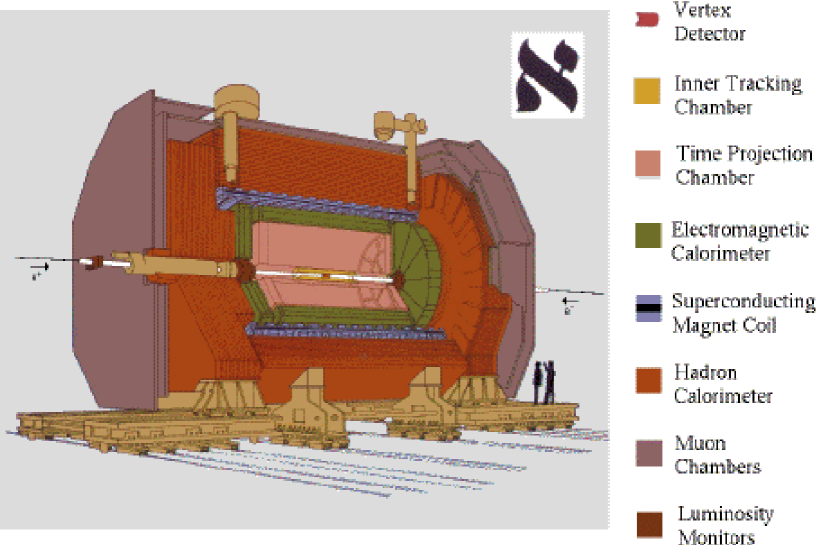
Figure 3.1: The ALEPH detector.

Particles produced at the IP and travelling outwards through the detector first encounter a series of three, low-density tracking subdetectors designed primarily to give information on the trajectories of charged particles. Since the tracking volume lies within a strong magnetic field, the curvature of a charged particle’s path through the field yields its momentum. They then reach a high-density calorimeter arrangement designed to bring them to rest and, in doing so, make a measurement of their energy. Any particles that manage to penetrate this, pass finally through the muon chambers designed to tag muons leaving the detector. The magnetic field is produced by a superconducting coil located between the electromagnetic and hadron calorimeters, and runs parallel to the beam-axis with a strength of 1.5 T.

The Cartesian ($x$, $y$, $z$) coordinate system used to describe positions within ALEPH is defined as follows. The origin is the geometrical centre of the detector, also the nominal IP. The $z$-axis runs parallel to the beam-pipe in the e^- beam direction. The $x$-axis points towards the centre of LEP (to the right as seen by an incoming positron), while the $y$-axis points vertically upwards. A cylindrical ($r$, $\phi$, $z$) coordinate system is also used, in which the origin and $z$-axis coincide with those of the Cartesian system. The planes $\phi=0^{\circ}$ and $\phi=90^{\circ}$ contain the $x$-axis and the $y$-axis respectively, and $r=\sqrt{x^{2}+y^{2}}$. In addition, it is often useful to refer to the angle made between the line that joins a point to the origin and the $z$-axis, and this is denoted by $\theta$.

A detailed description of the performance of the ALEPH detector is available in [28]. It should be noted that ALEPH has been undergoing constant modification over the years it has been operating, from minor changes too slight to be of note, to major changes like the replacement of the vertex detector in 1995. This analysis however, is only concerned with the data-taking period, 1997 onwards. Only the state of the detector in this period is described here, and when this state differs from previous years this will not necessarily be noted. With this in mind, there now follows a detailed description of the main components of ALEPH.

3.3 The Vertex DETector (VDET)

The VDET is the innermost subdetector of ALEPH. It is a silicon-strip detector which provides high-accuracy positional information on the paths of charged particles close to the IP both in the $r\phi$ plane and the $z$ direction. This allows accurate determination of their trajectories in this region and thus gives information on the point of origin of a charged particle, whether that be from the IP or not. This is of course most useful for the study of B-physics, allowing the accurate reconstruction of the decay vertices of B-mesons close to the IP.

The active part of the VDET is made up of 24 ‘faces’ arranged in two, approximately cylindrical layers. The inner layer consists of 9 faces and is at the lowest possible radius allowed by the presence of the beam-pipe ($\sim 6.3\,\mathrm{cm}$), the outer consists of the remaining 15 and is at the greatest possible radius allowed by the presence of the Inner Tracking Chamber ($\sim 10.3\,\mathrm{cm}$) - thus maximising the lever arm. The faces overlap by $\sim 0.2\,\mathrm{mm}$ in $r\phi$ to ensure complete coverage.

The active units of the VDET are the ‘wafers’, these are double-sided silicon strip detectors of size 52.6 $\mathrm{mm}$ $\times$ 65.4 $\mathrm{mm}$ $\times$ 0.3 $\mathrm{mm}$. Essentially junction diodes operated in reverse bias, each is an n-type substrate with 1021 p+ readout strips on the junction ($r\phi$) side and 640 orthogonal readout n+ strips on the ohmic ($z$) side. The passage of a charged particle through the wafer generates ionisation which is picked up as signal by nearby strips. Clusters of signals are combined using a ‘centre-of-gravity’ algorithm to produce VDET hits.

Three wafers and a support for the readout circuits all glued together form a ‘module’, two modules mounted with their readouts at opposite ends on two beams form a face, active length 400 $\mathrm{mm}$, total length 500 $\mathrm{mm}$. One beam is made of Kevlar epoxy and serves to electrically insulate the z side of the modules, the other is made of Carbon fibre epoxy and provides the necessary mechanical strength of the face. The faces are then mounted at each end on carbon fibre support flanges, which are joined together by a carbon fibre cylinder which sits between the two active layers and consists of two thin skins spaced 20 $\mathrm{mm}$ apart by a corrugated web. The whole support structure is water cooled. The readout cables and water pipes are supported by a second pair of 20 $\mu\mathrm{m}$ thick aluminium flanges, joined by two 200 $\mu\mathrm{m}$ thick carbon fibre cylinders which serve both to support the flanges and as inner and outer protective skins for the VDET. Figure 3.2 shows a cross-section of the completed structure in the rz plane and the face geometry as seen in the r$\phi$ plane, Figure 3.3 shows details of a face as seen from above and below and a three dimensional view of the fully mounted VDET.

Figure 3.2: Cross-sections of the VDET showing structural composition in the $rz$ plane (left) and face geometry in the $r\phi$ plane (right).

Figure 3.3: A VDET face (left) and the fully mounted VDET (right).

A charged particle passing through a face well inside its active region stands a 99% chance of leaving a reconstructed hit in both the $r\phi$ and z views. The chance of that hit being assigned to its reconstructed track in one view when it has been assigned in the other, giving a three-dimensional hit for the track, is 93% for the $z$ view and 95% for the $r\phi$ view. The spatial hit resolution for primary tracks at $\theta=90^{\circ}$ is 10 $\mu\mathrm{m}$ in the $r\phi$ view, with no significant change for decreasing $\theta$, and 15 $\mu\mathrm{m}$ in the $z$ view, worsening to 50 $\mu\mathrm{m}$ by $|\cos(\theta)|=0.85$. The 40 $\mathrm{cm}$ active length of the VDET (virtually) guarantees at least one hit up to $|\cos(\theta)|=0.95$.

3.4 The Inner Tracking Chamber (ITC)

The ITC is a cylindrical wire drift-chamber providing tracking information in the region $26\,\mathrm{cm}>r>16\,\mathrm{cm}$ and $|z|<100$ $\mathrm{cm}$. It has a fast readout allowing it to be used in the Level-1 trigger decision and provides the only tracking information used in that decision. For a charged particle passing through its full active thickness it can provide eight hits with a resolution of $\sim 150$ $\mu\mathrm{m}$ in $r\phi$ but only $\sim 5\,\mathrm{cm}$ in $z$.

The wires are strung parallel to the $z$-axis between two 25 $\mathrm{mm}$ thick aluminium end-plates. The end-plates themselves are connected by two carbon fibre tubes which form the cylindrical surfaces of the ITC. The outer tube bears the tension of the wires, and has an inner radius 57 $\mathrm{cm}$, a thickness of 2 $\mathrm{mm}$, and has a 25 $\mu\mathrm{m}$ layer of aluminium foil on both surfaces to screen the chamber from RF interference and improve the uniformity of its field. The inner tube, which provides support to the VDET, is 600 $\mu\mathrm{m}$ thick with a 50 $\mu\mathrm{m}$ thick layer of aluminium foil on its outer surface for the same reason. The high voltage is supplied by distribution boxes mounted on electrical end-flanges 20 $\mathrm{cm}$ beyond the end-plates. These end-flanges plus the cylinders form a hermetically sealed volume which contains a gas mixture of four parts argon to one part carbon dioxide at atmospheric pressure.

There are four different types of wire. The sense wires, responsible for attracting the ionisation produced by passing charged particles, are held at a positive potential of $\sim 2$ kV. Each is surrounded by five field wires and a calibration wire all held at ground potential, forming a hexagonal ‘drift cell’ (see Figure 3.4). Between each pair of drift cell layers is a layer of guard wires, these support circular hoops of aluminium wire whose purpose is to limit the damage that would be caused should any wire break. There are 96 sense wires per layer in the first four layers, and 144 per layer in the outer four layers.

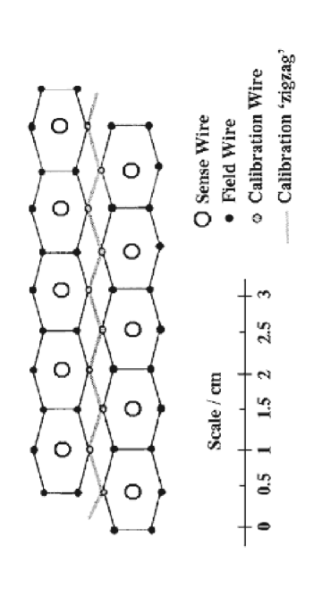
Figure 3.4: A detail of an ITC end-plate (left) and the drift cell geometry (right).

An ITC hit is created when a charged particle passes through a drift cell. Its passage ionises the gas in its immediate vicinity causing a pulse of negative charge to drift to the sense wire. The subsequent current pulse is detected at both ends. The distance of the particle from the wire is obtained by converting the drift time into a drift distance using a parameterisation of the non-linear relationship between the two. ITC hits have an inherent $r\phi$ ambiguity due to the azimuthal symmetry of the drift cells, the result of which is that each hit can represent one of two points on either side of the relevant sense wire. This ambiguity can be removed in practice since drift cells of neighbouring layers are offset from each other by half a cell width, thus only the correct set of possible hit points will line up to form a valid track. The $z$ coordinate of a hit is obtained from the difference in the time of arrival of the pulse at each end of the sense wire. Note that no more than one hit can be assigned to each wire in a given event.

3.5 The Time Projection Chamber (TPC)

The TPC is ALEPH’s main tracking chamber. It accurately measures the trajectories of charged particles by providing three-dimensional hits at 21 separate radii in the range $170\,\mathrm{cm}>r>40\,\mathrm{cm}$ and $|z|<220$ $\mathrm{cm}$. It also measures the spatial rate of energy loss due to ionisation ($\mathrm{d}E/\mathrm{d}x$) of a particle, which enhances particle identification by complementing information from the calorimeters. Structurally, the TPC consists of three main elements - the field cage (two cylinders, inner and outer), two circular end-plates and eight ‘feet’ (four attached to each end-plate, they transmit the weight of the whole structure, plus that of the ITC, to the magnet cryostat). A diagram is shown in Figure 3.5.

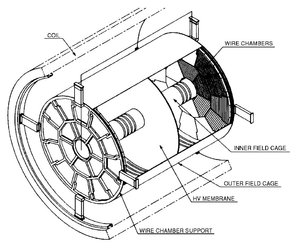
Figure 3.5: TPC overall view.

The cylindrical field cage is aligned with the $z$-axis and has an inner radius of 31 $\mathrm{cm}$ and an outer radius of 180 $\mathrm{cm}$. This, together with the end-plates, forms the gas-tight volume of the TPC which contains a mixture of argon (91%) and methane (9%) held at slightly above atmospheric pressure. The volume is vertically bisected by a circular mylar membrane coated in conducting graphite paint and held at a high negative voltage (typically $-27$ kV). The end-plates are held near ground while electrodes along the inner and outer field cages are held at potentials such that the resulting electric field (of $\sim$115 Vcm^-1) is uniform and aligned with the $z$-axis.

A charged particle passing through the volume ionises the gas along its path, and the electric field causes the resulting electron cloud - an image of the particle’s trajectory - to drift towards the nearest end-plate, while its lateral diffusion is limited by the parallel magnetic field.

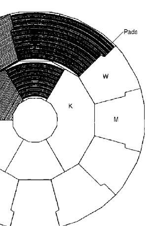
Figure 3.6: Overall geometry of a TPC end-plate showing sectors, wires and the 21 concentric pad rows.

The end-plates are divided into ‘sectors’ which are the active detecting regions. Each is a proportional wire chamber over a series of concentric ‘pad’ rows. The pads, 6.2 $\mathrm{mm}$ $\times$ 30 $\mathrm{mm}$ ($\delta$r$\phi$ $\times$ $\delta$r), provide the three-dimensional hit coordinates, while the wire chambers provide the $\mathrm{d}E/\mathrm{d}x$ information. A diagram of an end-plate showing the sector, wire and pad geometry can be seen in Figure 3.6. There are three different sector types (M, W and K). Significant dead regions, 24 $\mathrm{mm}$ wide, exist between neighbouring sectors’ radial boundaries such that any portion of a particle’s path in r$\phi$ that lies over a dead region will not produce hits. As such, the relative geometry of the three sector types was chosen such that the dead regions zigzag, limiting the number of hits a particle can lose in this way.

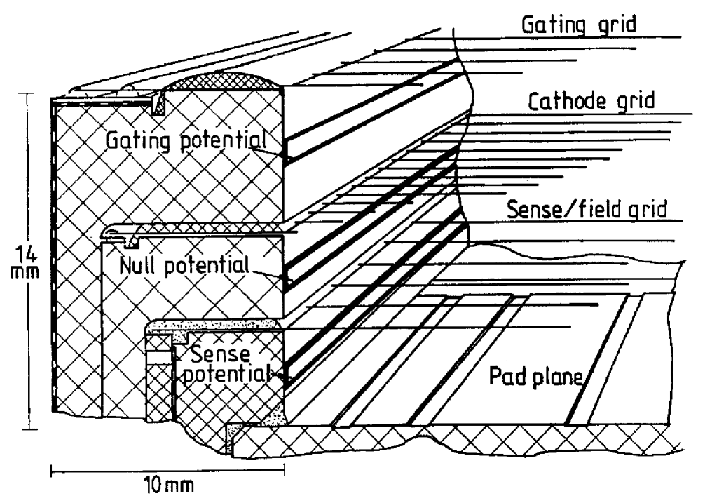
Figure 3.7: Schematic diagram of a sector edge showing wires and pads. The strips on the left are held at potentials such as to reduce field distortions at sector boundaries.

Ionisation from a particle’s path arriving at the end-plate encounters first a layer of wires called the gating grid (see Figure 3.7). If the Level-1 trigger has reached a ‘yes’ decision this will be held at a potential such that it is transparent to the passage of ionisation. Next it will encounter the cathode grid which is held at null potential to provide a shield between the uniform field of the main TPC volume and the field produced by the third and final layer. This is the sense grid and consists of alternating sense and field wires, the sense wires being held at null potential while the field wires are held at a high positive potential. As a result, incoming electrons avalanche towards the sense wires. The time of arrival and profiles of the resulting charge pulses are measured both by the sense wires and, through capacitive coupling, by the nearby pads.

The integrated charge of each wire pulse is proportional to the $\mathrm{d}E/\mathrm{d}x$ of the particle multiplied by the length of the particle’s path that projects onto the wire. They are recorded and are used to calculate the $\mathrm{d}E/\mathrm{d}x$ of each track once reconstruction has taken place. Clusters of pad pulses form the ($r$, $\phi$, $z$) TPC hits. Pad pulses which have multiple peaks in their time-profile are split, allowing more than one pulse per pad and thus ultimately, hits that overlap in $r\phi$. The radius of a hit comes simply from the radius of the relevant pad row (clusters do not transcend rows). The $\phi$ value comes from a combination of the $\phi$’s of the relevant pulses, although the exact nature of the combination depends on the number of pulses involved. The $z$ value is calculated from the cluster time using the drift velocity, the cluster time being a charge-weighted average of the time-of-arrival estimates of the pulses. The drift velocity is known from laser calibration.

A single-hit resolution of 173 $\mu\mathrm{m}$ in $r\phi$ and 740 $\mu\mathrm{m}$ in $z$ has been measured from leptonic $Z^{0}$ decays (which involve few, high momentum tracks leading to clear, accurately reconstructed events). Average resolution decreases with particle momentum and dip angle (as such, two-photon events have about the worst resolution).

The fractional momentum resolution, which is proportional to momentum, was measured from ideal $Z^{0}\rightarrow\mu^{+}\mu^{-}$ events. For tracks reconstructed purely from TPC hits it was found to be

$$\frac{\Delta p}{p^{2}}=1.2\times 10^{-3}\,\mathrm{GeV}^{-1}.$$

With the benefit of ITC hits this drops to

$$\frac{\Delta p}{p^{2}}=0.8\times 10^{-3}\,\mathrm{GeV}^{-1},$$

and with VDET hits, to

$$\frac{\Delta p}{p^{2}}=0.6\times 10^{-3}\,\mathrm{GeV}^{-1}.$$

3.6 Material density within the tracking volume

Clearly, from the point of creation of a particle to its entrance into the calorimeters, any interaction with the material of the detector is undesirable since it will alter the particle’s 4-vector and so corrupt its measurement. Such interactions can also create new particles which may be confused with those resulting from the physics at the interaction point. This would be especially problematic close to the beam axis where information about a particle’s momentum, or even existence before an interaction would be minimal or non-existent. An ideal tracking device would therefore be transparent to the particles passing through it, i.e. of zero density. Obviously this is not achievable in the real world where the amount, distribution and density of material comprising a subdetector can only be minimised within the constraints of the design criteria of that subdetector, both as a measuring device of sufficient accuracy and as a physical structure of sufficient strength.

The principal high-density components that exist within the ALEPH tracking volume are summarised in Table 3.1, and it is these that are responsible for the vast majority of material interactions at non-negligible polar angles. Most of this material is necessary to isolate the various gas systems that exist within ALEPH, i.e. the virtual vacuum of the beam-pipe, the argon-carbon dioxide mixture of the ITC and the argon-methane mixture of the TPC. The total number of radiation lengths of material to be penetrated by a straight particle from the interaction point before reaching the first VDET layer and first TPC pad are shown in Figures 3.8 and 3.9 respectively as a function of polar angle. The former is important since the first VDET layer is the first active part of the detector that a particle will typically encounter. Any interaction that happens at a lower radius happens ‘in the dark’, corrupting the relevant particle’s 4-vector before it has a chance even to be detected. Also, any new particles that are created as a result of the interaction will be more difficult to reject since they will not be lacking any hits. The amount of material before the first TPC pad is of interest since there is no more solid matter between here and the outer edge of the tracking volume. Figure 3.9 then serves as a summary of the problematic material listed in Table 3.1 as a function of polar angle, and shows that a high-energy photon emitted from the IP with $\theta=90^{\circ}$ stands a 6% chance of pair-converting before entering the TPC. Note that in general, as the polar angle decreases, the thickness of material to be penetrated increases, due to the decreasing angle of incidence into cylindrical components of the detector. Peaks and lumps are due to circular end-plates and non-cylindrical support structures.

Component Purpose Material Geometry Thickness Radiation (or principal (mm) lengths materials if many) (% of X₀) Beam-pipe Holds LEP vacuum & Be Cylinder, 1.1 0.3 supports VDET $r=5.3\,\mathrm{cm}$ VDET Active subdetector Si, Complex, see N/A 1.5 + support structure carbon fibre sect.3.3 & Araldite ITC inner wall Contains ITC gas & Carbon Cylinder, 0.6 0.3 supports VDET fibre $r=12.8\,\mathrm{cm}$ ITC end-plates Contain ITC gas & Al Holed discs, 25 28 transmit wire tension $30\,\mathrm{cm}>r>12.8$ $\mathrm{cm}$, to outer wall $z=\pm 100$ $\mathrm{cm}$ ITC outer wall Contains ITC gas & Carbon Cylinder, 2 1 counters wire tension fibre $r=28.5\,\mathrm{cm}$ TPC inner wall Contains TPC gas Al, mylar Cylinder, 10.5 2.3 & forms inner & Nomex $r=31\,\mathrm{cm}$ electric field cage honeycomb

Table 3.1: A summary of the principal high-density components within the tracking volume. Numbers quoted in the geometry column give the inner surface of the component.

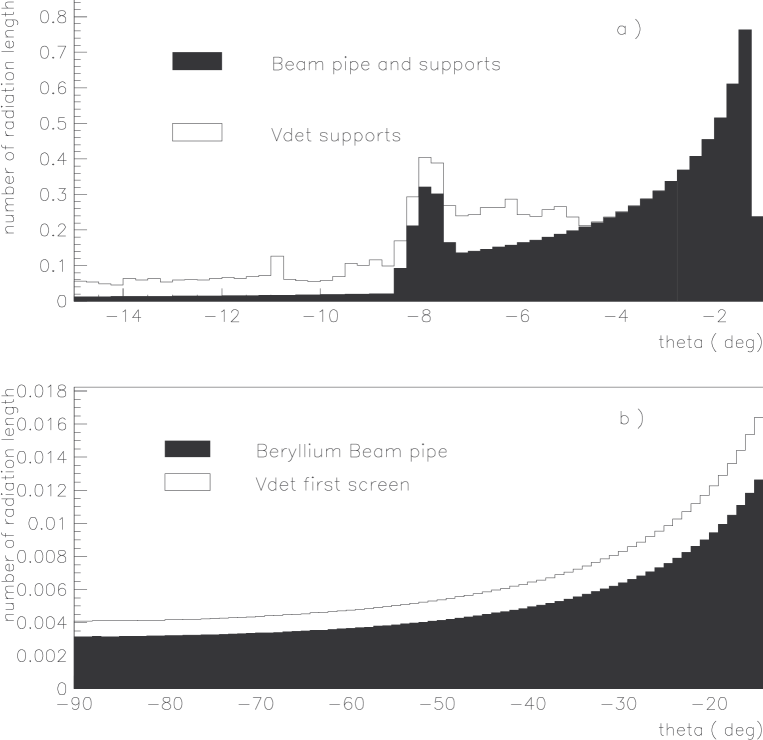
Figure 3.8: Material before the first VDET layer as a function of polar angle, $\theta$.

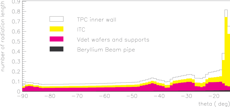
Figure 3.9: Material before the first pad of the TPC as a function of polar angle, $\theta$.

3.7 The Electromagnetic CALorimeter (ECAL)

The ‘ECAL’ is a lead and wire chamber sampling calorimeter with a thickness of 22 radiation lengths. It performs a multi-stage energy measurement of electromagnetic particles. Opaque to electrons and photons, it can yield their total energy. Hadrons and muons typically penetrate its full thickness. In measuring both the transverse and longitudinal shower profiles created by particles it also provides information on particle identity.

Again, it is comprised of a barrel plus two endcaps aligned with the $z$-axis. Each is segmented into twelve modules in $\phi$. A module (there is little difference whether it be in the barrel or an endcap) is a hermetically sealed unit containing 45 ‘layers’ in an 80%-xenon to 20%-carbon dioxide gas mixture held at slightly above atmospheric pressure. A layer consists of a lead sheet, an aluminium extrusion containing an anode wire plane, and a plane of cathode pads separated and insulated from the wires by a graphite-coated mylar layer (see Figure 3.10). An incoming photon or charged particle will generate an electromagnetic shower upon collision with the lead sheet. Electrons freed by the resulting ionisation of the gas are avalanched towards the anode wires where the resulting charge pulse capacitively induces a signal on nearby cathode pads (each measuring $30\,\mathrm{mm}\times 30\,\mathrm{mm}$). Thus the pads measure the position of the e.m. showers whilst the wires, which have a fast readout, can be used in the trigger. The 45 layers of a module are split into three ‘stacks’. The first stack contains the first 10 layers and is 4 radiation lengths thick, the second contains the next 23 and is 9 radiation lengths thick, the third contains the final 12 and is also 9 radiation lengths thick since its lead sheets are double the thickness (4 $\mathrm{mm}$ as opposed to 2 $\mathrm{mm}$). Cathode pads from consecutive layers are grouped and connected internally into ‘towers’, which are skewed such as to point to the IP. Energy deposits from all pads belonging to a particular stack within a tower are summed in readout. This provides three energy readings per tower, the magnitudes of which (absolute and relative) depend on the incoming particle ID and energy.

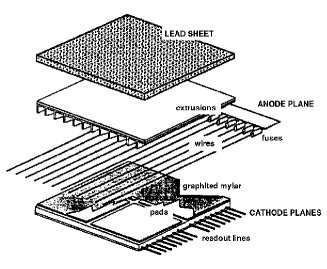
Figure 3.10: Portion of a separated ECAL layer.

In excess of 73,000 towers provide the high granularity required for good $e\!-\!\pi$ separation in jets. Solid angle coverage is $3.9\pi$ with dead regions due to module boundaries representing 2% of the barrel surface and 6% of the endcap surface. Endcap and barrel modules are offset from each other by 15^∘ to prevent coincidence of boundaries. Calibration over the full energy range is performed using Bhabha, $\tau$$\tau$ and $\gamma$$\gamma$ events, and also independently of any events using radioactive sources mounted close to the gas inlets and injected periodically into the gas system. The fractional energy resolution, $\Delta$E/E, for electrons and photons is $(18\,\mathrm{GeV}^{\frac{1}{2}}/\sqrt{E})$%. The spatial resolution is $(6.8\,\mathrm{mm}\,\mathrm{GeV}^{\frac{1}{2}}/\sqrt{E}$).

3.8 The Hadron CALorimeter (HCAL)

The HCAL forms the final barrier to particles travelling through the detector, and is designed to stop hadrons and provide a measure of their energy. Muons typically penetrate its full thickness, and their departure from the detector is tagged by muon chambers surrounding the main body of the HCAL. A particle at normal incidence encounters 1.2 $\mathrm{m}$ of iron, equivalent to 7.2 interaction lengths for hadrons. The HCAL also serves as the main support structure of ALEPH, and as the return path for the magnetic field.

It consists of a barrel of twelve modules and two endcaps of six modules each. A module consists of 22 consecutive layers of 5 $\mathrm{cm}$-thick iron and streamer tubes, and is typically $\sim 7\,\mathrm{m}$ long depending on position. Each has a final layer of 10 $\mathrm{cm}$-thick iron. The tubes consist of 8 $\mathrm{cm}$-wide ‘comb’ profile PVC extrusions contained in plastic boxes. Nine ‘teeth’ form eight cells, each containing an anode wire running the length of the tube in a gas mixture of 22.5% Ar to 47.5% CO₂ to 30% isobutane. A photograph is shown in Figure 3.11. The internal surfaces of the cells are coated in graphite paint. Showers from collisions in the iron layers create ionisation in the tubes, and the resulting electrons avalanche towards the anode wires. Signals are induced on cathodes on both sides of the tube. The upper (open) side supports copper pads, the lower supports aluminium strips which run the length of the tube. Like the ECAL, the pads are grouped into towers pointing to the IP. There are just under 2,700 towers in all, and the angular ($\Delta\phi\times\Delta\theta$) size they present to the IP ranges from $3.7^{\circ}\times 3.0^{\circ}$ at $\theta=90^{\circ}$, to $15.0^{\circ}\times 2.5^{\circ}$ at $\theta=6^{\circ}$. The aluminium strips are 4 $\mathrm{mm}$ wide. Their output is binary, indicating whether or not a tube has been fired at least once. They provide a detailed two-dimensional view of shower propagation within the detector which is important for muon identification.

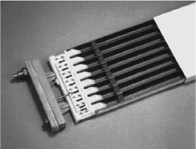
Figure 3.11: Photograph of a streamer tube.

Surrounding the iron structure are two double layers of tubes, 50 $\mathrm{cm}$ apart around the barrel, 40 $\mathrm{cm}$ apart at the endcaps. These are the muon chambers. Here the pad layers are replaced by additional strip layers which run orthogonally to the tubes, enabling three-dimensional hits to be obtained for charged particles leaving the detector. Together with information from the main bulk of the detector this provides powerful muon identification.

The energy resolution of the HCAL for pions is $\Delta E/E=(84\,\mathrm{GeV}^{\frac{1}{2}}/\sqrt{E})$%.

3.9 The Luminosity CALorimeter (LCAL)

The LCAL is a lead and wire chamber sampling calorimeter which provides the main luminosity measurement for ALEPH. An accurate measurement of the luminosity is essential in order to obtain reaction cross-sections from event-rates. The measurement is obtained from the event-rate of the QED t-channel Bhabha process, which is well understood. The differential cross-section is proportional to $\theta$^-4, and receives corrections due to interference from the s-channel process, e⁺e^-$\rightarrow$Z/$\gamma$$\rightarrow$e⁺e^-, which decrease with $\theta$. Thus in order to obtain the high event-rates needed for an accurate measurement of the luminosity, and to make insignificant the s-channel corrections, the LCAL sits at very low $\theta$.

The LCAL consists of two annuli about the beam-pipe, 25 radiation lengths thick, beginning at $z=\pm 263$ $\mathrm{cm}$. Each covers the range 44 mr to 160 mr and is formed by two semi-annular modules with 38 sampling layers each. The modules are almost identical to ECAL modules, with layers consisting of lead and proportional wire chambers (see Figure 3.10). Like the ECAL, the layers are grouped into three stacks, and pads are grouped into towers which point to the IP. There are 384 towers per module.

Bhabha events are tagged by requiring back-to-back hits in both units above a threshold energy. The integrated luminosity is obtained by dividing the number of events seen by the theoretical cross-section multiplied by the experimental efficiency. An accuracy of the order of 0.5% is obtained.

3.10 The trigger system.

Necessary to the operation of ALEPH is a system that will judge when an event of note (e⁺e^- annihilation, Bhabha or two-photon) has taken place and will subsequently initiate the readout of the subdetectors. This is the trigger system. It allows the TPC to exist in its insensitive state (‘gate closed’, see Section 3.5) for much of the running time without loss of efficiency. It also reduces the amount of uninteresting data written to tape, and the dead-time of the detector that results from readout.

The trigger decision is split into three levels, each based on increasingly more complex information. The Level-1 trigger reaches a conclusion within 5 $\mu\mathrm{s}$, less than the bunch crossing time. It requires a good charged track in the ITC and/or information from the calorimeters indicative of a particle deposit. Should the decision be ‘yes’, the TPC gate is held open and the Level-2 decision is processed within 50 $\mu\mathrm{s}$. This is essentially a recalculation of the Level-1 decision based now on three-dimensional information from the TPC. In the case of a ‘yes-decision’ readout of the whole detector is initiated, otherwise data-acquisition is halted and reset.

During LEP1 the Level-1 trigger performed much better than was anticipated, making Levels-2 and 3 relatively unimportant as they vetoed only a small fraction of events. Since running at LEP2 energies however, noisier beam conditions have led to a large increase in the number of unwanted background ‘events’. As a result the importance of Level-2 has risen greatly, now reducing the event-rate by in excess of 50%. Level-3 is an offline trigger, remains unimportant and is not described here.

3.11 Event reconstruction

Event reconstruction refers to the processing that is performed on the raw data output from the detector in order to correlate the information and produce final data that is more representative of what actually occurred in the event. Most important from the point of view of the analysis described in this thesis, is the track reconstruction. The tracks are the reconstructed helical trajectories of the charged particles and are formed by connecting the hits produced in the tracking chambers. The reconstruction algorithm starts in the TPC, linking nearby hits to form track segments. Segments which are compatible with a single helical trajectory with an axis parallel to the $z$-axis are connected to make tracks. At least four TPC hits are required for a track. These are then extrapolated down into the ITC and VDET where compatible hits are added. If there are ITC hits left unassigned to a track then the algorithm attempts in a similar way to form these into tracks (which will then not have assigned TPC hits). These tracks are required to have a minimum of four ITC hits. The tracks are parameterised by a set of five helix parameters. These are: the inverse radius of a track’s circular projection in the $xy$ plane, 1/$R$; the tangent of its ‘dip angle’ (equal to the ratio of its longitudinal and transverse momentum components), tan($\lambda$); its distance of closest approach to the $z$-axis, $\mathrm{d}_{0}$; and the ratio of its $y$ and $x$ momentum components and its $z$ coordinate at that point, $\phi_{0}$ and $\mathrm{z}_{0}$ respectively. A final track fit is performed using Kalman filter techniques [29].

Once an event is reconstructed, the energy flow algorithm is run. The purpose of this is principally to create associations between charged tracks and calorimeter deposits, enabling the identification of particles and an improvement in the overall energy resolution, and is described in detail in [30] and [28]. Unfortunately energy flow was not written with charged particle decay in the tracking volume in mind. It disregards tracks with a $\mathrm{d}_{0}$ greater than 2 $\mathrm{cm}$ or a $|\mathrm{z}_{0}|$ greater than 10 $\mathrm{cm}$, and so is of limited use in this analysis.

Chapter 4 The Search

4.1 Introduction

This thesis details a search for the supersymmetric process by which (lightest) neutralinos are pair-produced in $e^{+}e^{-}$ collisions, each then independently and promptly decaying to a slepton plus corresponding lepton, the sleptons then travelling a measurable distance in the detector before themselves decaying to a lepton plus gravitino.

$$e^{+}\ e^{-}\rightarrow\chi\ \chi\rightarrow\tilde{l}l\ \tilde{l}l\rightarrow\tilde{G}ll\ \tilde{G}ll$$

The final state is thus four leptons (two from the IP, two from kinks or with large $\mathrm{d}_{0}$) plus missing energy (since the gravitinos will not be detected). Each neutralino decays independently giving six distinct channels, $\tilde{e}\tilde{e}$, $\tilde{\mu}\tilde{\mu}$, $\tilde{\tau}\tilde{\tau}$, $\tilde{e}\tilde{\mu}$, $\tilde{e}\tilde{\tau}$ and $\tilde{\mu}\tilde{\tau}$. An example event is shown in Figure 4.1. This process can contribute to the exclusion of the GMSB parameter space (or potential for GMSB discovery) since, for a significant portion of the kinematically allowed space, the cross-section for the neutralino is greater than that for the slepton, and so when $m_{\chi}>m_{\tilde{l}}$, slepton production via neutralino decay can dominate over direct production.

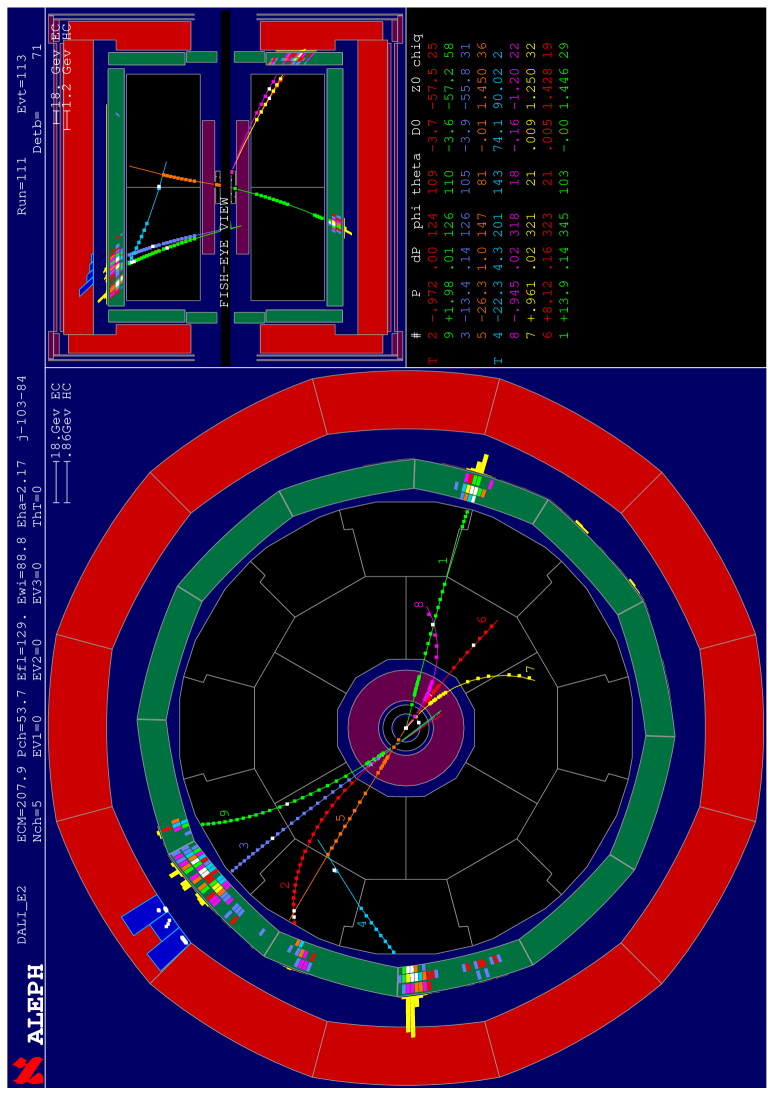
Figure 4.1: An example Monte Carlo $\tilde{e}\tilde{\tau}$ event at 208 $\mathrm{GeV}$. The detector is shown in the ‘fish-eye’ view to magnify the tracking volume relative to the calorimeters. The $\tilde{\tau}$ decayed after travelling a few centimeters, the $\tilde{e}$ after travelling $\sim 1\,\mathrm{m}$. Both $\tau$’s have undergone three-prong decay.

The ultimate goal of the search was to discover evidence for supersymmetry. In the absence of any such evidence, it was to formulate model-independent cross-section limits for the process and to exclude as much of the kinematically allowed parameter space as possible under a minimal GMSB model.

The search was performed using a total of 628 $\mathrm{pb}$^-1 of LEP2 data taken over a range of centre-of-mass energies from 189 to $208\,\mathrm{GeV}$, recorded between 1998 and 2000 (see Table 4.1). The data was stored on ‘DST’s. These contain all the information about the reconstructed ALEPH events (unlike the usual format of MINIs), but events must fulfil some basic criteria to be written to DST from ‘POT’ (essentially the same but containing all events). An event must have

• more than $3\,\mathrm{GeV}$ of charged energy coming from within 5 $\mathrm{cm}$ in $\mathrm{d}_{0}$ and 20 $\mathrm{cm}$ in $\mathrm{z}_{0}$

• OR 2 or more charged tracks with $\mathrm{d}_{0}$ and $\mathrm{z}_{0}$ within this range

• OR total ECAL wire energy greater than 15 $\mathrm{GeV}$ and ECAL $|t_{0}|<500$ $\mathrm{ns}$ ($t_{0}$ is the difference between the time of the event as recorded by the ECAL wires and the time of the nearest LEP bunch crossing: events due to conventional $e^{+}e^{-}$ collision typically have $|t_{0}|<100$ $\mathrm{ns}$)

• OR 1 or more photon candidates and no charged tracks.

A method was required to distinguish events from the process being searched for (‘signal’ events) from events due to known Standard Model processes (‘background’ events). The technique used is called Monte Carlo analysis, and requires the simulation of both the signal and the background. The simulated events are called Monte Carlo data. The method for distinguishing signal from background can then be developed using the Monte Carlo data, and subsequently applied to the real data. The results can be compared to the results that would be expected in the absence of the signal as given by the background Monte Carlo, and the degree of evidence for the signal process can be quantified.

Energy (GeV) Year Integrated Luminosity (pb^-1) 188.6 1998                 174. 2 191.6 1999 29. 0 195.5 1999 79. 9 199.5 1999 86. 3 201.6 1999 41. 9 199.8 2000 0. 8 201.8 2000 0. 7 202.7 2000 1. 8 203.8 2000 8. 3 205.0 2000 71. 6 206.3 2000 65. 5 206.6 2000 60. 8 208.0 2000 7. 3 Total = 628. 0

Table 4.1: Integrated luminosities recorded by ALEPH at each centre-of-mass energy achieved by LEP between 1998 and 2000. Year 2000 energies formed a continuum and have been placed in 1 $\mathrm{GeV}$ bins about integer values. The energy shown is the luminosity weighted average.

4.2 Monte Carlo simulation

4.2.1 Signal

Signal Monte Carlo data was produced using SUSYGEN 2.2 [31] before subsequent processing by GALEPH [32] (the ALEPH detector simulation program based on GEANT [33],[34]) and JULIA [35] (the ALEPH event reconstruction program used to reconstruct both Monte Carlo and real data events). The sleptons were set stable at generator level, then tracked and decayed by GALEPH.

The characteristics of a signal event as observed in the detector depend only on the neutralino mass, and the slepton masses and lifetimes. GMSB dictates that either the sleptons are degenerate in mass, and therefore share the role of the NLSP (the co-NLSP scenario), or that the stau is lighter and so is the sole NLSP (the stau-NLSP scenario). In the first case the mass degeneracy also leads to lifetime degeneracy, and so all three sleptons are described by a single mass and a single lifetime. In the second case the mass difference between the stau and the selectron/smuon becomes an extra free parameter. But it is of little importance since if the stau is significantly lighter than the selectron/smuon then the neutralino will decay almost exclusively to it, and so no channel other than the $\tilde{\tau}\tilde{\tau}$ is of importance and the mass of the selectron/smuon is irrelevant. Thus although GMSB parameter space is six-dimensional, the working parameter space for this search can be reduced to three dimensions, ($m_{\chi}$, $m_{\tilde{l}}$, $\tau_{\tilde{l}}$), where $l$ can be $e$, $\mu$ or $\tau$ in the case of degeneracy, and $\tau$ otherwise. These are of course not the only relevant parameters. The neutralino production cross-section and branching ratios are of critical importance to the success of the search since they define the event rates for each channel. But for the purposes of signal Monte Carlo generation and the formulation of the selections they are not important.

For the purposes of Monte Carlo generation it is necessary to identify the approximate region of parameter space in which the selections are likely to be sensitive. In particular, slepton lifetimes should be chosen such that a good mapping of the variation of the selection efficiency with slepton lifetime is obtained over the region of interest. Thus it is natural to convert slepton lifetime to slepton decay length, since this is the principal feature of the signal events, and thus will have a far more direct relationship to the selection efficiencies. The natural working parameter space is then ($m_{\chi}$,$m_{\tilde{l}}$, $d_{\tilde{l}}$), where $d_{\tilde{l}}$ is the slepton decay length in the detector. At the time of Monte Carlo generation, sensible values can be chosen for the slepton decay length based on the detector size and geometry, and then translated into slepton lifetimes ensuring a good efficiency mapping. The slepton decay length is a function of $m_{\chi}$, $m_{\tilde{l}}$, $\sqrt{s}$ as well as $\tau_{\tilde{l}}$. In general this function is not simple because the ionisation caused by the slepton as it passes through the material of the detector will cause it to slow down, and so the decay length is also a ‘function’ of the detector set-up. However, it is not necessary that the translation from decay length to lifetime be exact, and the following approximation is used:

$$\tau_{\tilde{l}}=\frac{d_{\tilde{l}}}{\gamma\beta c}$$

where,

$$\gamma\beta=P_{lab}/m_{\tilde{l}}\ ,$$

$$P_{lab}=\sqrt{E_{rest}^{2}-m_{\tilde{l}}^{2}+\left(E_{rest}\ p_{\chi}/m_{\chi}\right)^{2}}\ ,$$

$$E_{rest}=(m_{\chi}^{2}+m_{\tilde{l}}^{2}-m_{l}^{2})/2m_{\chi}\ ,$$

$$p_{\chi}=\sqrt{E_{beam}^{2}-m_{\chi}^{2}}\ .$$

Here $\gamma$ and $\beta$ pertain to the slepton in the lab frame, $P_{lab}$ is the (initial) momentum of the slepton in the lab frame if it is emitted at 90^∘ to the lab direction in the neutralino rest-frame, $E_{rest}$ is the energy of the slepton in the neutralino rest-frame, $p_{\chi}$ is the momentum of the neutralino in the lab frame, $E_{beam}$ is the LEP beam energy and $m_{l}$ is the mass of the relevant lepton. In the case of a mixed channel (i.e. the two sleptons have different flavours) the lifetime is calculated with both lepton masses and the average is taken.

Initial work showed that for a given decay length, the selection efficiencies were only weak functions of the neutralino and slepton masses. Thus Monte Carlo data was generated to focus on the variation of selection efficiency with decay-length more than on the masses. Eight decay-lengths were chosen, and seven points in ($m_{\chi}$, $m_{\tilde{l}}$) space were generated for each of them, apart from the two highest decay lengths for which an extra two points in mass space were used (since some initially surprising results were obtained for long decay lengths which will be described in Section 7.2), making a total of sixty points. This was done for each channel at both the lowest and the highest LEP centre-of-mass energies under consideration: 189 $\mathrm{GeV}$ and 208 $\mathrm{GeV}$. An exception was the $\tilde{e}\tilde{e}$ channel at 189 $\mathrm{GeV}$ which was used as a test case, and so 21 mass points were generated per decay length. 500 events were generated at each point. The slepton masses ranged from 67 $\mathrm{GeV}$ to 102 $\mathrm{GeV}$  and the neutralino masses from 69 $\mathrm{GeV}$ to 103 $\mathrm{GeV}$  with never less than a 1 $\mathrm{GeV}$ mass difference between them. The decay lengths ranged from 2 $\mathrm{mm}$ to 20 $\mathrm{m}$. The exact points at which Monte Carlo data was generated for each channel at each energy are given in Appendix A. Slepton mass degeneracy was always assumed in the generation of the mixed channels ($\tilde{e}\tilde{\mu}$, $\tilde{e}\tilde{\tau}$, $\tilde{\mu}\tilde{\tau}$).

All the signal Monte Carlo data was run through the POT $\rightarrow$ DST selection described in Section 4.1, and events failing were appropriately tagged and not included in any signal efficiencies.

4.2.2 Background

Due to the nature of the signal a large array of Standard Model processes form significant backgrounds to the search. Only processes which are very easily cut against, or which have a very low cross-section can be disregarded as sources of background. A list of the backgrounds analysed, together with their cross-sections, the number of events that were analysed, and the generators used for their production, is given in Table 4.2. At 189 $\mathrm{GeV}$ (at which 174 $\mathrm{pb}$^-1 of data was collected) roughly 20 times the number expected in data were analysed for each process. At 208 $\mathrm{GeV}$ (at which only 7.3 $\mathrm{pb}$^-1 of data was collected) roughly 200 times the number expected in data were analysed for each process. These factors were not achieved for the two-photon to tau and up/down quark processes however, since limited Monte Carlo samples were available.

Process At 189 $\mathrm{GeV}$ At 208 $\mathrm{GeV}$ Generator $\sigma$ (pb) No. analysed $\sigma$ (pb) No. analysed Annihilation $qq$ 99.4 340,000 78.8 120,000 KORALZ 4.2 $\tau\tau$ 8.21 30,000 6.61 10,000 KORALZ 4.2 $WW$ 16.6 60,000 17.5 26,000 KORALW 1.21 $ZZ$ 2.76 10,000 2.79 4,000 PYTHIA 5.7 $Zee$ 99.1 350,000 98.9 144,000 PYTHIA 5.7 Two-photon $\gamma\gamma\rightarrow\tau$ 431 800,000 461 600,000 PHOT02 $\gamma\gamma\rightarrow ud$ 487 400,000 487 250,000 PHOT02 $\gamma\gamma\rightarrow c$ 93.2 160,000 94.4 50,000 PHOT02 $\gamma\gamma\rightarrow s$ 23.9 40,000 23.7 17,000 PHOT02

Table 4.2: The Standard Model background processes that were analysed as backgrounds to the search. $\sigma$ is the production cross-section. The final states of annhilation processes are created via the annihilation of the electron and positron, whereas the final states of two-photon processes are created via the collision of two photons which originated from the electron and positron. For information about KORALZ, KORALW, PYTHIA and PHOT02 see [36], [37], [38] and [39] respectively.

The generated events were processed by GALEPH and JULIA in the same way as for signal. Kinematic cuts were applied in the generation of the two-photon Monte Carlo data. For all the stated two-photon processes, events were required to have a final state invariant mass greater than $2.5\,\mathrm{GeV}$. For the two-photon to tau process, final states were required to have at least $0.15\,\mathrm{GeV}$ of transverse momentum. For the two-photon to quark processes a scattering angle of at least 5 mr was required for the electron or positron.

The samples were split into two equal halves, one to act as a guide in formulating the selections, the other to give the final background expectation once the selections were finalised (so as to minimise bias in the background expectation). Exceptions were the two-photon to quark processes where the high cross-section and limited Monte Carlo samples meant that the same sample had to be used for both.

Chapter 5 Event Analysis

5.1 Introduction

The technique for the selection of candidate signal events is a two-step process. Firstly, using the ALPHA [40] package which facilitates access to the full event information, preliminary data candidates are identified using some simple preselection. For those events satisfying the preselection, variables are calculated that are designed to be sensitive to the differences between signal and background. These are written to HBOOK [41] ntuples (essentially tables of data in which rows correspond to successive events and columns correspond to variables) forming a greatly reduced data set. The second stage is the application of a selection, consisting of a set of cuts on the variable values, to determine the final signal candidates. This is the technique used by most searches for physics beyond the Standard Model at LEP.

Many, if not all, of the variables should pertain to the event as a whole, such as the number of charged tracks, total energy and invariant mass. In order to calculate such ‘global’ variables the relationships between the various reconstructed detector objects such as tracks and calorimeter deposits should be known. This is the purpose of the energy flow algorithm. But energy flow has only limited abilities to make sense of processes that are happening away from the interaction point. It ignores tracks with a $\mathrm{d}_{0}$ greater than 2 $\mathrm{cm}$ or a $\mathrm{z}_{0}$ greater than 10 $\mathrm{cm}$, and since JULIA does not reconstruct the slepton decay vertex, it does not recognise the relationship between the reconstructed slepton track (if there is one) and the resulting lepton track. Thus energy flow will only yield correct results if the slepton decay length is short enough for the resulting lepton to satisfy the cuts on $\mathrm{d}_{0}$ and $\mathrm{z}_{0}$, or long enough for the slepton to reach the calorimeters before decay; and so it is of limited use in this analysis.

Even if energy flow did treat charged particle decay in the tracking volume correctly, the signal would still not be well-defined by global variables in the case of the $\tilde{\tau}\tilde{\tau}$ channel (and the $\tilde{e}\tilde{\tau}$ and $\tilde{\mu}\tilde{\tau}$ channels to a lesser extent) because of the larger number of invisible particles (up to eight neutrinos on top of the two gravitinos) and the larger range in the charged track multiplicity (from multi-prong tau decays). The selection then relies primarily on the presence of high-$\mathrm{d}_{0}$ tracks: that being the primary feature of the signal. Several other processes can generate high-$\mathrm{d}_{0}$ tracks though, such as nuclear interactions, ECAL splash-backs, photon conversions, multiple scattering and cosmic rays. The frequency with which these processes occur means that their rejection efficiency must be close to 100% if they are not to swamp any signal.

After the event preselection is described in Section 5.2, this chapter goes on to detail the procedures that are used to discriminate between high-$\mathrm{d}_{0}$ tracks due to the signal process, and those due to background. Sections 5.3 and 5.4 describe the identification of ECAL splash-backs and nuclear interactions respectively. Then Section 5.5 describes the procedure that is used to confirm (or reject) that a high-$\mathrm{d}_{0}$ track is compatible with the hypothesis of originating from slepton decay. The final cut-based selections are described in Chapter 6. In order to facilitate the descriptions of the procedures described in this chapter a terminology is used which is explained below and in Figure 5.1. The figure also introduces some points of interest concerning tracks reconstructed from particles that have not been produced at the IP. There are three terms which are important to understand:

The post(pre)-$\mathrm{d}_{0}$ trajectory of a particle. This is the section of the particle’s trajectory after it has passed (before it has reached) its point of closest approach to the beam-axis.

A post(pre)-$\mathrm{d}_{0}$ track. This is a track that has been formed by hits created on the post(pre)-$\mathrm{d}_{0}$ portion of a particle’s trajectory. Both this and the term above refer to truths about the event that are not known a priori from the reconstructed information.

The post(pre)-$\mathrm{d}_{0}$ section of a track. This is the section of a track which is post(pre)-$\mathrm{d}_{0}$ according to the track direction (assigned by JULIA, and which may be incorrect). The track will only have assigned hits on its post-$\mathrm{d}_{0}$ section. If it is a pre-$\mathrm{d}_{0}$ track then its pre-$\mathrm{d}_{0}$ section will probably follow closely the post-$\mathrm{d}_{0}$ section of a post-$\mathrm{d}_{0}$ track (see Figure 5.1).

Although this terminology might seem confusing, it is an unfortunate reflection of the subtleties involved in the relationship between the reconstructed and ‘truth’ information of tracks not originating from the IP.

Many of the procedures involve the fitting of tracks to vertices, either to test whether a group of tracks form a new vertex, or whether they fit to an existing vertex. This is performed using the ALEPH YTOP package described in [42] and [43]. It provides a $\chi^{2}$ for each fit performed, which is normalised to the number of degrees of freedom.

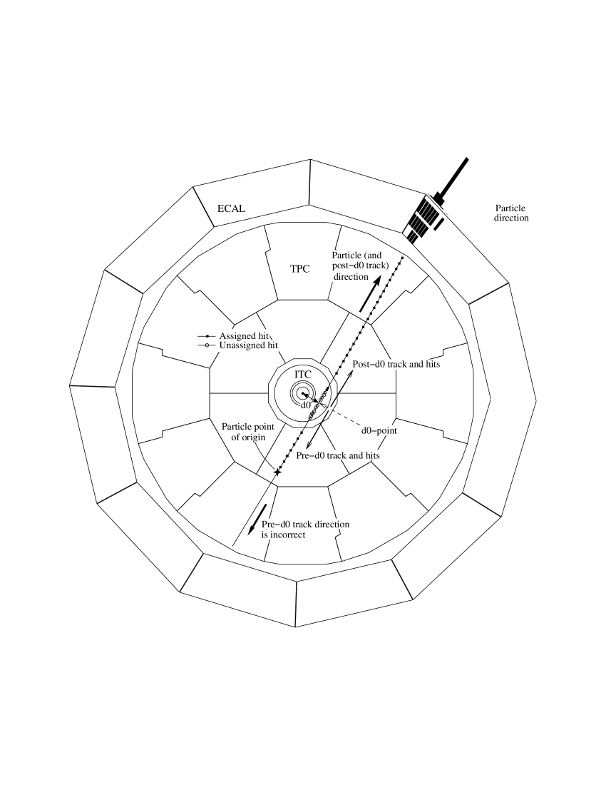
Figure 5.1: The reconstructed track(s) of a particle that has been produced in the TPC, moving towards the beam-axis, through the ITC, then back out into the TPC and on to the ECAL. The $\mathrm{d}_{0}$-point is the point at which the track is closest to the beam-axis. Before it reaches the $\mathrm{d}_{0}$-point it is travelling along its pre-$\mathrm{d}_{0}$ trajectory, afterwards, along its post-$\mathrm{d}_{0}$ trajectory. Since the idea that particles are produced at the IP is a paradigm within JULIA, it assumes that the particles responsible for all tracks were moving away from the beam-axis and did not originate significantly before their $\mathrm{d}_{0}$-point. For this reason it will not form tracks from hits that would lie on both sides of the $\mathrm{d}_{0}$-point; and so the particle trajectory shown here is reconstructed as two tracks: one pre-$\mathrm{d}_{0}$ track reconstructed from the pre-$\mathrm{d}_{0}$ hits, and one post-$\mathrm{d}_{0}$ track reconstructed from the post-$\mathrm{d}_{0}$ hits. JULIA incorrectly assigns the directions of pre-$\mathrm{d}_{0}$ tracks as being radially outwards, and so both their momentum 3-vector and charge have the wrong sign. Tracks that have no TPC hits will be referred to as ITC tracks, tracks that do have TPC hits will be referred to as TPC tracks and may or may not have ITC hits. Either type of track may or may not have VDET hits.

5.2 Preselection

In order to speed up analysis, events were first subjected to some very basic preselection aimed at fast rejection of events that were clearly not signal candidates. The event was rejected if

• The scalar sum of the momenta of all tracks was less than $4\times(E_{LEP}/188.6)\,\mathrm{GeV}$ (to reduce the number of two-photon events)

• The total number of tracks was less than 3 or greater than 30 (to reduce both two-photon and $q\overline{q}$ events)

• The total number of tracks was less than 4 and the two highest momentum tracks had momenta greater than half the beam energy and the angle between them was greater than $179^{\circ}$ (to reduce $e^{+}e^{-}$ and $\mu^{+}\mu^{-}$ events)

• The total number of energy flow charged tracks was greater than 11 (to further reduce $q\overline{q}$ events)

• The energy flow event energy was less than $7\times(E_{LEP}/188.6)\,\mathrm{GeV}$ and the energy flow event momentum was less than $1\times(E_{LEP}/188.6)\,\mathrm{GeV}$ (to further reduce two-photon events)

5.3 Rejection of ECAL splash-backs

The electromagnetic shower created when a charged particle enters the electromagnetic calorimeter typically propagates in the direction of the incoming particle. Some of the electrons and positrons in the shower can however, scatter back into the TPC where they can be reconstructed as tracks. This is known as an ‘ECAL splash-back’.

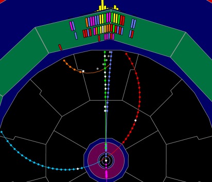
Figure 5.2: An example of an ECAL splash-back in a Monte Carlo $\tau\tau$ event at $189\,\mathrm{GeV}$. Two electrons have escaped the ECAL to be reconstructed as high $\mathrm{d}_{0}$ tracks in the TPC, one arcs through the ITC and passes out the other side to form a third track.

They are characterised by a high-$\mathrm{d}_{0}$ track ‘entering’ the ECAL (in fact the particle responsible is leaving but JULIA assumes all tracks move radially away from the beam-axis: the track is pre-$\mathrm{d}_{0}$) close to another track that has higher momentum, with both forming a common vertex in the region of the ECAL (see Figure 5.2 for an example). The only circumstance under which this is likely to occur in a signal event is when the slepton decays inside the ECAL and the resulting lepton is ejected back into the TPC. Since this analysis is only intended to be sensitive to slepton decay in the tracking volume then the possibility of rejecting signal events by confusing slepton decays with ECAL splash-backs is not regarded a problem.

The track that results from the splash-back will be referred to as the output track, the track causing the splash-back will be referred to as the input track. The conditions that must be satisfied by both a candidate output and input track for the output track to be tagged as a splash-back are as follows:
• The output track must have TPC hits and momentum, $p_{output}<\\ 5\times(E_{LEP}/188.6)\,\mathrm{GeV}$ and $\mathrm{d}_{0}$$>0.5\,\mathrm{cm}$ or $\mathrm{z}_{0}$$>2\,\mathrm{cm}$. • The input track must also have TPC hits and have $p_{input}>0.5\,\mathrm{GeV}$ and $p_{input}>p_{output}$. • The points at which the output and input tracks leave the TPC volume must be within 50 $\mathrm{cm}$ of each other. • The tracks must form a common vertex in the region $165<r<230\,\mathrm{cm}$ and $|z|<300\,\mathrm{cm}$, or $200<|z|<300\,\mathrm{cm}$ and $r<230\,\mathrm{cm}$ (these roughly correspond to the vicinity of the ECAL barrel and endcaps respectively).

5.4 Rejection of nuclear interactions

Hadrons interacting with nuclei in the structure of the detector can cause hadronic showers leading to multiple high-$\mathrm{d}_{0}$ tracks. These are characterised by many tracks originating from a common vertex which is displaced from the IP (see Figure 5.3 for an example). Like splash-backs these have distinct characteristics that can be tagged. Care must be taken though to avoid confusing a $\tilde{\tau}\rightarrow\tau_{multi-prong}$ decay vertex with a nuclear interaction.

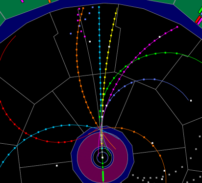
Figure 5.3: An example of a nuclear interaction in a Monte Carlo $\tau\tau$ event at $189\,\mathrm{GeV}$. A pion from the decay of a tau has interacted with a nucleus in the inner TPC wall, giving a shower of high-$\mathrm{d}_{0}$ tracks, mainly protons.

Clearly an algorithm that can find multiple tracks originating from a common vertex is required. Initially this was done by testing all track pairs for compatibility with a common vertex, and then attempting to merge these 2-track vertices. This was very CPU intensive however, and a method which used the fitting routine less often was sought. The procedure settled upon relied on starting with a single high-$\mathrm{d}_{0}$ track, and trying to add further tracks to it to build up a multi-track vertex. Once all the tracks that could be added had been (which may be none at all), and if there were one or more other high-$\mathrm{d}_{0}$ tracks in the event which had not been included in the vertex, then one of these was used in the same way as the first track to try to build a new vertex. Unlike the first method tried, this method required making a choice as to the order in which the tracks should be selected so as to give the best chance of all tracks from a given vertex actually being included. Using tracks in order of increasing fractional momentum error was found to be successful. The exact procedure used is shown in the flow diagram of Figure 5.4. In this diagram ‘most reliable’ means smallest fractional momentum error. A track passes ‘basic cuts’ if it has not been tagged as an ECAL splash-back, has TPC hits, has a momentum smaller than half the beam energy and greater than $0.1\,\mathrm{GeV}$, and a $\mathrm{d}_{0}$$>0.15\,\mathrm{cm}$ or a $\mathrm{z}_{0}$$>3\,\mathrm{cm}$. A track is ‘hit-compatible’ with a vertex if at least all bar one of its hits lie on one side of the vertex, so that it is compatible with the hypothesis that it was produced at that vertex.

Figure 5.4: Flow diagram showing the procedure used to find and tag nuclear interaction vertices.

Once one multi-track vertex has been found with this procedure, then if each new vertex after the first is less than $3\,\mathrm{cm}$ from, or shares more than 50% of its tracks with, a previously found vertex then an attempt is made to merge the two. If this results in a new vertex with a $\chi^{2}$ (given by YTOP) less than 70 then the merge is considered successful, and the two vertices are replaced with the single merged vertex.

Once the vertices have been finalised, certain properties are calculated for each, such as the summed momentum and charge of the constituent tracks. Care was taken however, to account for a potentially problematic feature of the reconstruction algorithm. Since JULIA always assumes that particles move radially away from the beam axis, a particle that is produced far enough from the beam axis and moving back towards it can result in two reconstructed tracks (a pre-$\mathrm{d}_{0}$ and a post-$\mathrm{d}_{0}$), as is shown in Figure 5.1. In this case the track corresponding to the portion of the particle trajectory before it reaches its point of closest approach to the beam axis is assigned the wrong direction. Thus its momentum 3-vector and charge have the wrong sign, and this will corrupt the overall properties of any multi-track vertex in which it is included. Also, since the total number of tracks in the vertex is used to classify it, then a single particle giving two tracks would corrupt this as well. To correct this, any track whose TPC hits lie at a smaller radius than the vertex has its charge and momentum 3-vector reversed. Then the $\mathrm{d}_{0}$, $\mathrm{z}_{0}$ and directions of these tracks are compared with any tracks which are part of the same vertex and for which the vertex lies on the pre-$\mathrm{d}_{0}$ portion. If the tracks differ in $\mathrm{d}_{0}$ and $\mathrm{z}_{0}$ by less than 30% of their respective average, and the angle between them at their $\mathrm{d}_{0}$-points is greater than $170^{\circ}$, then both are assumed to have originated from the same particle trajectory and the one with fewer TPC hits is removed from the vertex. As an example, if both the tracks shown in Figure 5.1 were found to originate from a nuclear interaction, then the pre-$\mathrm{d}_{0}$ track would be removed.

Each vertex is then placed into one of 3 categories based on its properties. A vertex is labelled as a $\tilde{\tau}\rightarrow\tau_{multi-prong}$ vertex if it satisfies all of the following conditions –

• its charge is $\pm 1$

• its largest two-track angle at the vertex is less than $20^{\circ}$

• its momentum is $>4\times(E_{LEP}/188.6)\,\mathrm{GeV}$ and $<55\times(E_{LEP}/188.6)\,\mathrm{GeV}$

• its kink-angle is between $5^{\circ}$ and $170^{\circ}$

• its kink-angle is $>15^{\circ}$ or its $|\cos(\theta)|$ is less than 0.6

• its number of tracks is less than 6

• its distance from the IP is greater than $0.3\,\mathrm{cm}$

• and its distance from the IP is greater than $1\,\mathrm{cm}$ or its $\chi^{2}$ is less than 3.

The charge of the vertex is the sum of the charges of all the constituent tracks. The momentum is the vector sum of the momentum 3-vectors of all the constituent tracks. The kink-angle is the angle between the vertex momentum 3-vector and the straight line from the IP to the vertex. The $|\cos(\theta)|$ of the vertex refers to the vertex position, i.e. $|z_{vertex}/\sqrt{r_{vertex}^{2}+z_{vertex}^{2}}\,|$.

Although this is a reasonably stringent set of cuts, background events can still have vertices labelled as $\tilde{\tau}\rightarrow\tau_{multi-prong}$ since a charged particle emitting a bremsstrahlung photon which quickly undergoes pair-conversion can create something very similar.

If a vertex fails this selection then it is classified as a nuclear interaction vertex if –

• its radius is greater than $4.8\,\mathrm{cm}$ (a nuclear-interaction is highly unlikely inside the beam-pipe, so the minimum radius is set at the beam-pipe radius of 5.3 $\mathrm{cm}$, minus 5 $\mathrm{mm}$ leeway)

• its largest two-track angle at the vertex is greater than $20^{\circ}$

• and its number of tracks is greater than 2.

If it fails this also then it is classified as ‘unknown’, and the constituent tracks are still considered valid.

5.5 Confirmation of slepton-decay hypothesis

Although this analysis attempts to reject high-$\mathrm{d}_{0}$ tracks from known sources such as those discussed in Sections 5.3 and 5.4, and these attempts are largely successful, they are not sufficient. The number of residual high-$\mathrm{d}_{0}$ tracks is still too many. Hence a procedure was developed, not to test whether a high-$\mathrm{d}_{0}$ track comes from a known background process, but to test whether it is compatible with coming from the signal process, i.e. the decay of a heavy charged particle. The hits of a candidate track are examined to identify the region of its length over which the responsible particle could have originated, and this is then used to calculate what can be expected as the detector response to the parent slepton. In the absence of such a response the track can be rejected. For instance, if a track’s hits indicate that the responsible particle must have been produced far out in the TPC, the parent slepton should have its own reconstructed track which forms a good kink-vertex with the high-$\mathrm{d}_{0}$ track. In the absence of such a 2-track vertex the high-$\mathrm{d}_{0}$ track can be rejected. This section describes the exact procedure in detail. It should be noted that only tracks that have TPC hits, a momentum greater than $1\,\mathrm{GeV}$, a $\mathrm{d}_{0}$ greater than $0.1\,\mathrm{mm}$ and a $\chi^{2}_{BS}$ (the $\chi^{2}$ of the track-fit to the beam-spot per degree of freedom) greater than 5 are considered as candidate high-$\mathrm{d}_{0}$ tracks.

5.5.1 A particle’s point of origin

While a reconstructed track is a reliable indicator of a particle’s trajectory, it does not tell us exactly where that particle originated or where it stopped/decayed. Nominally, the point of origin is considered to be the $\mathrm{d}_{0}$-point. This is fine for tracks originating from the IP, since the distance scale associated with the uncertainty on the particle’s exact point of origin will be at most the size of the beam spot, which will be several orders of magnitude lower than the track’s radius of curvature. Thus the track is effectively straight over the relevant range, and the uncertainty on its point of origin does not translate into significant uncertainty on its initial momentum 3-vector. For a track not originating from the IP no such simple assumption can be made, and only analysis of its hits can yield information as to its point of origin. This will take the form of a range of the track length over which the particle could have originated.

The following procedure for finding this range assumes that the track in question is post-$\mathrm{d}_{0}$ (i.e. reconstructed from hits created as the particle moves away from the beam axis), and so the track direction and charge are correctly assigned by JULIA. Although the following procedure is not sensible for a pre-$\mathrm{d}_{0}$ track, it will be explained later that such a track is in fact dealt with in the correct way.

The range over which the particle could have been produced is between the lowest-radius point at which there is evidence that the particle was following the track trajectory, and the highest-radius point at which there is evidence that it was not. To find evidence that the particle was not following the track trajectory, a scan is performed backwards along the track length, starting from the point at which it achieves its highest radius in the TPC, looking for missing hits. Nominally, a hit is expected at every TPC pad radius that the track crosses, every ITC wire radius that the track crosses while it is inside the ITC active volume, and every intersection that the track makes with a VDET wafer. There are several legitimate reasons why a track can be missing a hit however. The TPC sector boundaries form dead regions of the order of 1 $\mathrm{cm}$ wide, and in the ITC certain wires are not active. Also, even if the particle has produced a hit it may not be assigned to the respective track since the reconstruction algorithms can simply fail to assign the hits correctly, or may only have one hit to assign between two tracks (if they are closer than the minimum two-track resolution). Thus if the track fulfils any of the conditions given in Table 5.1 at a point where a hit is expected but not observed, the lack of a hit is not considered abnormal.

TPC $\bullet$ The track is $<$ 1.5 $\mathrm{cm}$ in $r\phi$ from a sector boundary $\bullet$ The track is $<$ 1.5 $\mathrm{cm}$ in $r\phi$ and $<$ 4 $\mathrm{cm}$ (10 $\mathrm{cm}$) in $z$ from another TPC (ITC) track on the same side (on either side) of the central membrane $\bullet$ The track is $<$ 2 $\mathrm{cm}$ in $r\phi$ and $<$ 4 $\mathrm{cm}$ in $z$ from an unassigned hit $\bullet$ The radius of the point in question is $<$ 3 $\mathrm{mm}$ greater than the
track’s $\mathrm{d}_{0}$ ITC $\bullet$ The nearest wire has a hit $\bullet$ The nearest wire is dead $\bullet$ The track is $<$ 1 $\mathrm{mm}$ in $r\phi$ from the cell edge and the next-nearest wire has a hit $\bullet$ The point in question is at a radius $<$ 0.1 $\mathrm{mm}$ above the track’s $\mathrm{d}_{0}$ VDET $\bullet$ There is a hit within 0.5^∘ in $\phi$ $\bullet$ The track is within one sigma of the wafer edge

Table 5.1: Conditions under which the lack of a hit is not considered abnormal in each tracking subdetector.

If a point is encountered at which there is no hit and at which none of the conditions of Table 5.1 are satisfied, then it is assumed that the responsible particle was not following the track trajectory at this point. Then if there are no hits at lower radii, the range for the particle point of origin is set between this point and the lowest-radius assigned hit. If there are one or more hits at lower radii, then the track information appears to be inconsistent with a genuine particle trajectory. In this case, if the point under consideration is in the VDET the track is rejected as bad. If it is in the ITC then the track is spared for now and the scan continues, but if another such point is encountered the track is rejected. If the point is in the TPC, then the location of the bad point is merely recorded. These bad TPC points will be referred to again later.

If the scan reaches the track’s $\mathrm{d}_{0}$-point without the track being rejected or the particle range-of-origin being determined then the scan continues along the pre-$\mathrm{d}_{0}$ section of the track, as far as the highest radius that the pre-$\mathrm{d}_{0}$ section of the track reaches in the TPC if necessary. On the pre-$\mathrm{d}_{0}$ section the track will not have any assigned hits and so Table 5.1 governs completely whether the track is considered good at each point. If the scan reaches the end of the pre-$\mathrm{d}_{0}$ section without conclusion, then the track is rejected (since it is probably a cosmic muon that has passed right through the detector).

5.5.2 Where is the slepton?

Once a range for the particle’s point of origin has been calculated, it is possible to translate this into a range of possible trajectories for the parent slepton, and to make the requirement that the event information supports one of these trajectories and thus the hypothesis that the candidate track originated from slepton decay. This section describes the procedure that is applied to do this.

There are four distinct scenarios for the reconstructed detector response to the slepton depending on how far the slepton travels before decay and in what direction. If the slepton achieves a high enough radius before decay it can produce a reconstructed TPC track, which should form a well-reconstructed vertex with the lepton track. In the following discussion this will be referred to as a TPC-vertex. Failing this, it can produce an ITC track which will form a vertex with the lepton track that is not so well reconstructed in $z$ due to the low $z$-resolution of the ITC. This will be referred to as an ITC-vertex. Failing this, if the slepton at least passes through some active tracking components before decay, then it should leave some hits which point to the lepton track. These will be referred to as pointing-hits. Finally there is the case that the slepton decays before creating any hits, and so the only sign of its existence is the $\mathrm{d}_{0}$ of the lepton track. Examples of each case are shown in Figure 5.5. The range for the point of origin of the particle responsible for the candidate high-$\mathrm{d}_{0}$ track determines which of these scenarios are possible, and which are not.

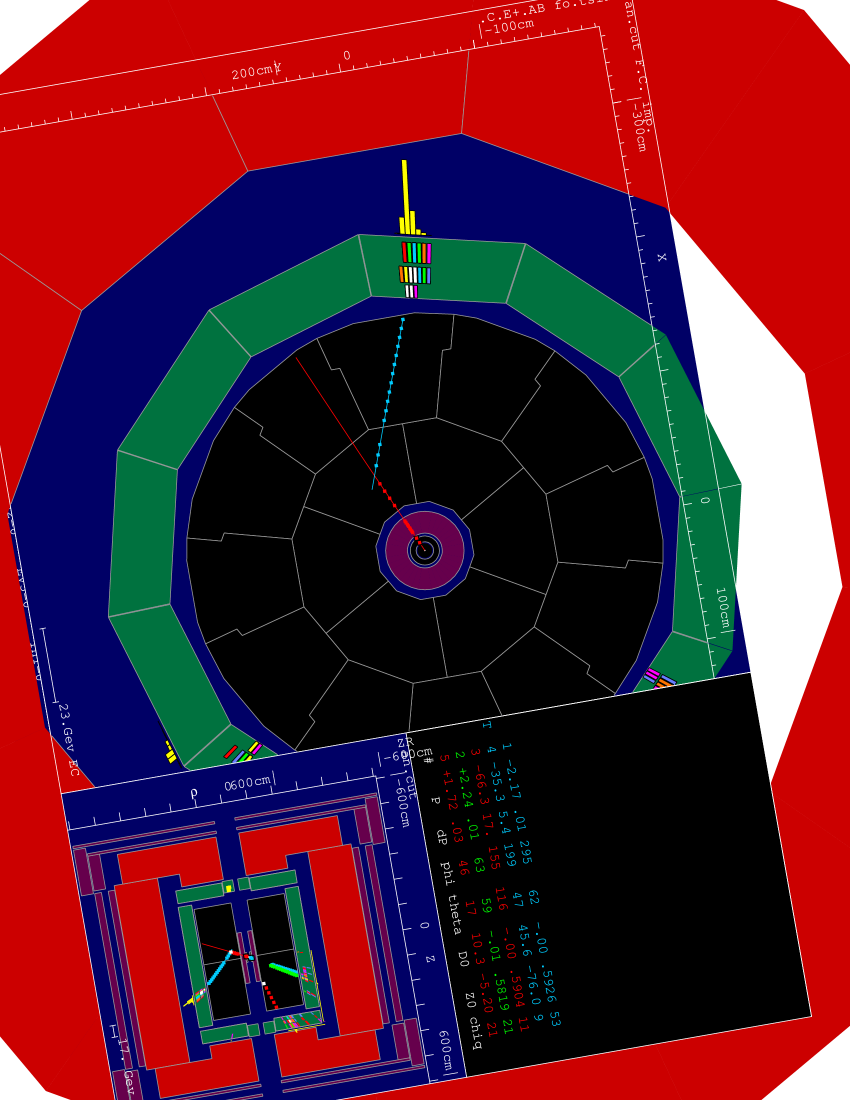
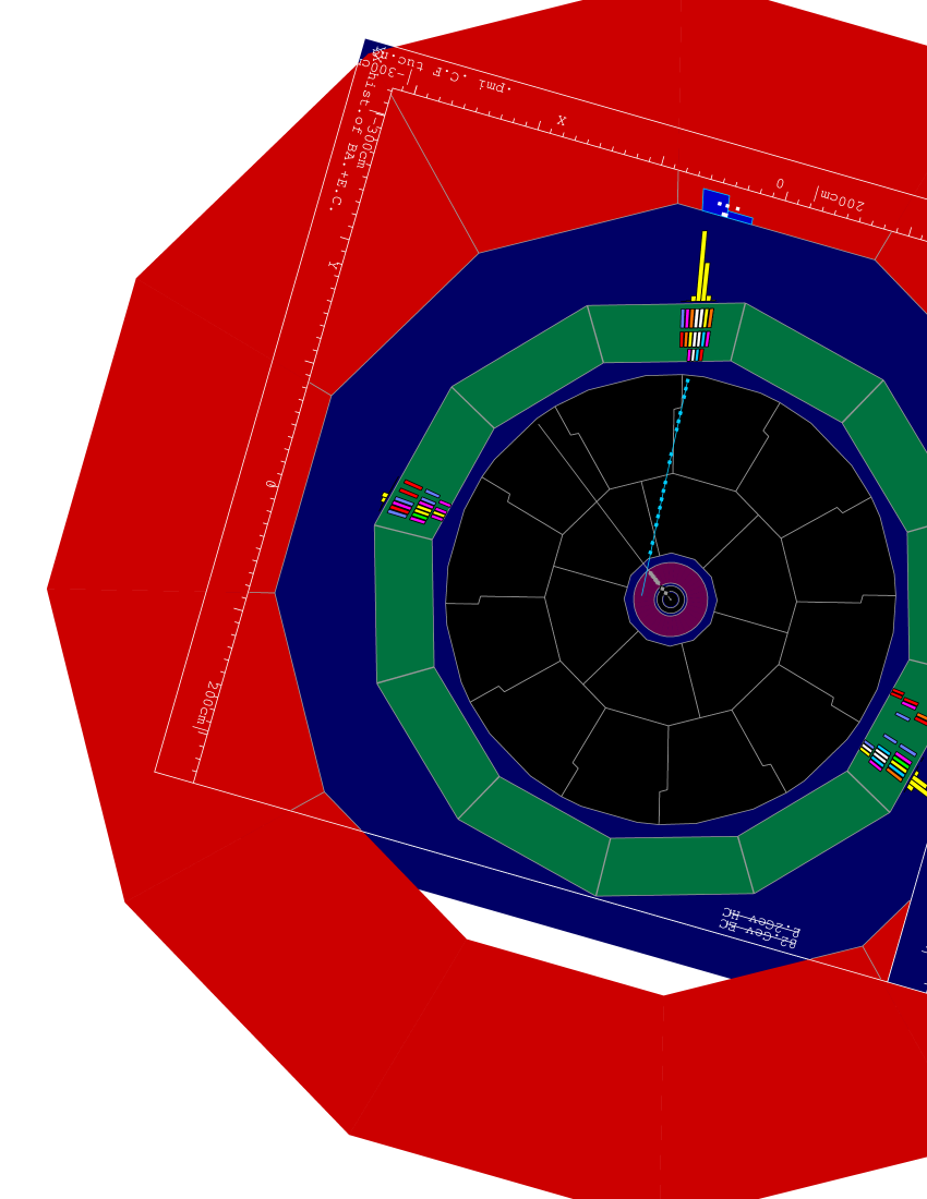
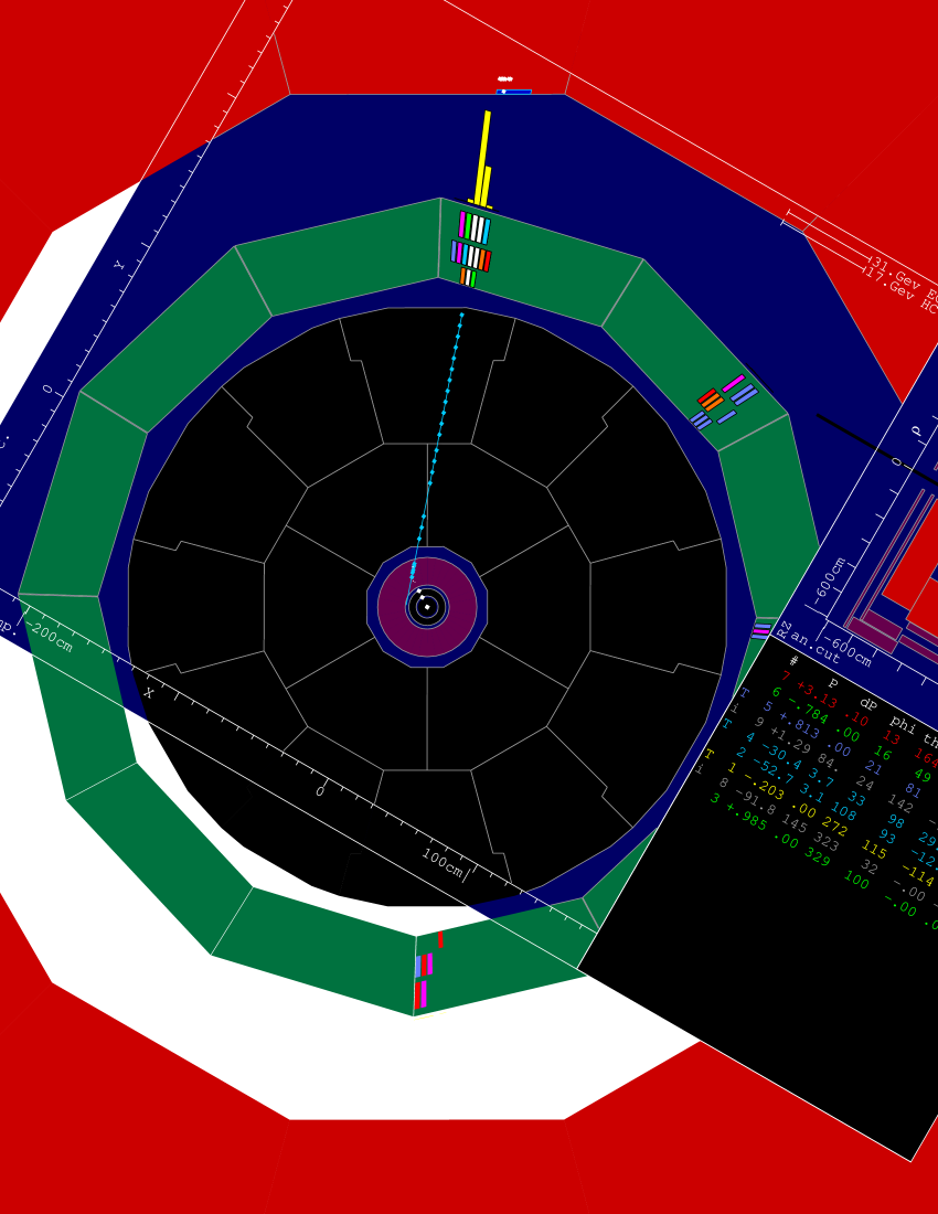
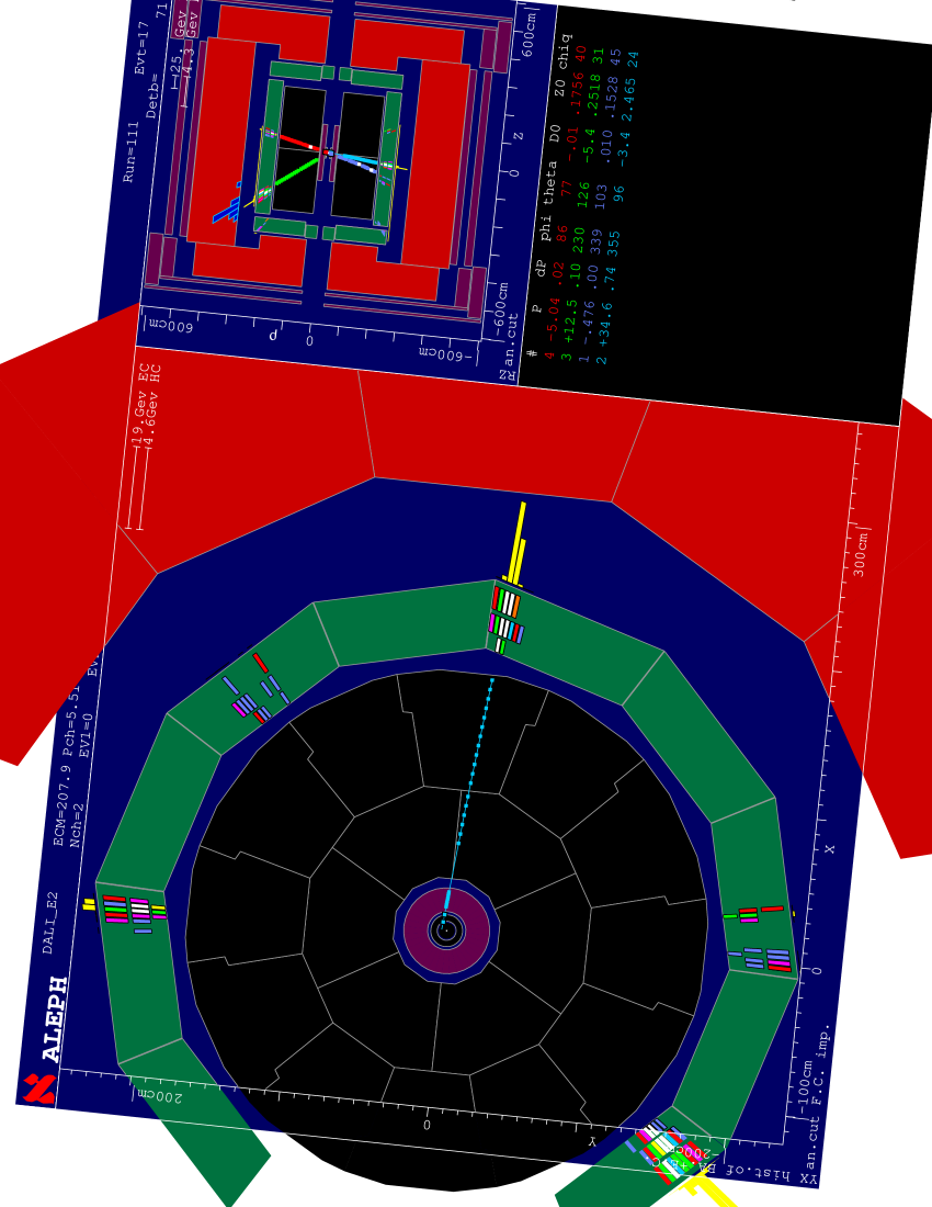
a). b). c). d).

Figure 5.5: Examples of the typical reconstructed detector response to the slepton and lepton for decreasing slepton decay lengths. Shown are (a) a TPC-vertex, (b) an ITC-vertex, (c) pointing-hits and (d) a simple high-$\mathrm{d}_{0}$ track from signal Monte Carlo data. All tracks and hits other than those of the slepton-lepton pair shown have been removed for clarity.

The relationship between the point of origin range and the possible scenarios is as follows. If, for at least part of the range,

• the track radius (i.e. the distance of the track from the $z$-axis) is above that of the 4th TPC pad row, then a TPC-vertex is possible.

• the track radius is above that of the 4th ITC wire layer and the track is either inside the ITC or the straight line from the track to the IP enters the ITC at a radius greater than this (and thus the slepton, under the assumption that its trajectory was straight, crossed at least 4 ITC wires), then an ITC-vertex is possible.

• the straight line from the track to the IP passes through some tracking components, then pointing-hits are possible.

• the straight line from the track to the IP passes through no tracking components, then no slepton response at all is possible.

These possibilities are not mutually exclusive, they could all be open. However, of those that are open, it may be possible to exclude some based on likelihood. For instance, if the track radius is significantly above that of the 4th TPC pad row for the entire range, then anything other than a TPC-vertex is unlikely, and a TPC-vertex can be demanded. Thus if any of these conditions, with $3\,\mathrm{cm}$ added to the radius necessary for a TPC-vertex and $3\,\mathrm{mm}$ added to the radius necessary for an ITC-vertex, are true over the entire range, then the first of the respective possibilities becomes a demand. If the demand is not satisfied, the track is rejected. If it is found that no single response can be demanded in this way, then the track is tested for the possible slepton responses in the order TPC-vertex, ITC-vertex, pointing-hits. If the track does not satisfy any of the possible responses (bearing in mind that if the case that the slepton did not produce any hits has been identified as a possibility, then no response is possible), then it is rejected.

The procedure involved in looking for TPC-vertices, ITC-vertices and pointing-hits will now be described.

TPC-vertices

The first step of testing a track for a TPC-vertex is to identify candidates for the slepton track. These are required to have TPC hits (by definition), a $\mathrm{d}_{0}$ less than $2\,\mathrm{cm}$ and a $\mathrm{z}_{0}$ less than $2.5\,\mathrm{cm}$, and must not have been identified as tracks from a nuclear-interaction or an ECAL splash-back. Its $\mathrm{d}E/\mathrm{d}x$ (if $\mathrm{d}E/\mathrm{d}x$ information is available for the track) must be no less than 10 standard deviations below that expected for a singly-charged particle of mass $60\,\mathrm{GeV}$ (the approximate GMSB slepton mass limit), and the track should show evidence that the particle responsible ceased to follow the track trajectory before leaving the TPC (i.e. be missing at least one hit from its end without observable reason – see Table 5.1). If there are no candidate slepton-tracks, there can be no TPC-vertices.

The high-$\mathrm{d}_{0}$ track is tested for a good TPC-vertex with each candidate slepton track. They must form a common vertex which lies on the post-$\mathrm{d}_{0}$ section of the slepton track and has a $\chi^{2}$ (from YTOP) less than 30. The $z$-coordinates of the two tracks at the vertex must differ by less than $7\,\mathrm{cm}$, the angle between them at the vertex must be greater than $10^{\circ}$, and the last assigned hit of the slepton track must not be at a radius more than $1\,\mathrm{cm}$ above that of the vertex.

The checks made on the high-$\mathrm{d}_{0}$ track’s hits are more complex, since there are three possibilities for their locations. If the decay-angle (defined here as the angle between the slepton and lepton directions at the point of decay in the $r\phi$ plane) is less than 90^∘ then all the high-$\mathrm{d}_{0}$ track’s hits lie at radii greater than the vertex radius, and both the track directions are correct and so the decay-angle will be calculated correctly (see Figure 5.5.a). If the decay-angle is greater than 90^∘ and the high-$\mathrm{d}_{0}$ track is post-$\mathrm{d}_{0}$, then again the track directions are correct and the decay-angle will be calculated correctly, but now the hits can lie both above and below the vertex radius so no constraints can be made on their positions (see Figure 5.6). However, if the decay-angle is greater than 90^∘ and the high-$\mathrm{d}_{0}$ track is pre-$\mathrm{d}_{0}$ (so all its hits lie at a radius smaller than that of the vertex), then the decay-angle will be calculated incorrectly to be less than 90^∘. So if the calculated decay-angle is less than 90^∘, all the hits are required to lie either at radii above that of the vertex minus 1 $\mathrm{cm}$, or at radii below that of the vertex plus 1 $\mathrm{cm}$. If the calculated decay angle is greater than 90^∘ then no constraints are made on the positions of the hits. Thus if a high-$\mathrm{d}_{0}$ track is found to have a TPC-vertex it can be tagged as post-$\mathrm{d}_{0}$ or pre-$\mathrm{d}_{0}$ based on the positions of its hits relative to the vertex.

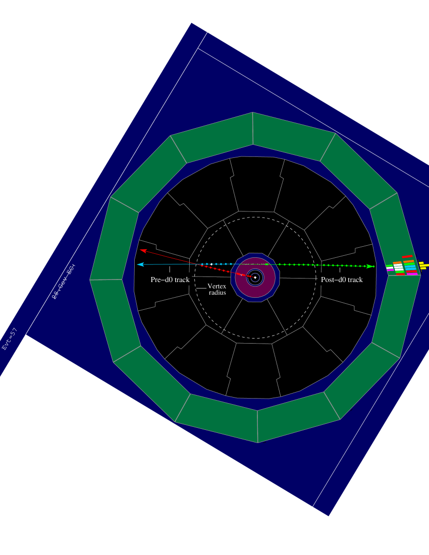
Figure 5.6: An example of a TPC-vertex with a decay angle greater than 90^∘. The lepton has formed a pre-$\mathrm{d}_{0}$ and a post-$\mathrm{d}_{0}$ track. The arrows show the track directions as assigned by JULIA.

At this stage, the number of bad TPC-points for the track (see Section 5.5.1) can be fixed. For pre-$\mathrm{d}_{0}$ tracks it is set as the number lying at least $6.5\,\mathrm{cm}$ (normal pad-row spacing plus $1\,\mathrm{mm}$) below the radius of the vertex. For post-$\mathrm{d}_{0}$ tracks it is the number lying above the radius. The number of bad TPC points forms a track variable which can be used as an indicator of the reliability of the track, and is referred to in the selections described in the next chapter.

ITC-vertices

As with TPC-vertices, the first step towards finding ITC-vertices is to identify candidate slepton tracks. These are required to have no TPC hits (by definition), a $\mathrm{d}_{0}$ less than $1\,\mathrm{cm}$ (no constraint on $\mathrm{z}_{0}$ due to the low ITC $z$-resolution) and a momentum greater than $1\,\mathrm{GeV}$.

The high-$\mathrm{d}_{0}$ track is then tested for a good ITC-vertex with each candidate slepton track. Because of the low $z$-resolution of the ITC a full vertex fit is not performed. It is merely required either that the tracks’ circular $r\phi$ projections cross in the $r\phi$ plane, in which case the crossing point closest to the beam axis is taken as the two-dimensional vertex, or that their distance of closest approach in $r\phi$ is less than $5\,\mathrm{mm}$, in which case the vertex position is the point of closest approach.

The vertex radius is required to be no more than $5\,\mathrm{mm}$ below that of the 4th ITC wire layer. The upper limit on the radius is determined by a scan along the ITC track outwards into the TPC, looking for evidence that the particle responsible was not following the track trajectory. At successive pad-row radii a set of conditions similar to those summarised in the TPC section of Table 5.1 are evaluated, with the $z$ requirements relaxed. The upper limit on the radius is then set at the radius of the second point at which the track is missing a hit without observable reason plus $5\,\mathrm{mm}$, unless the first and second points are consecutive in which case the first is used. The first point is in general not used since the track errors in the TPC are much greater in the absence of assigned TPC hits, and so some leeway is appropriate.

The ITC track is required not to have any assigned hits on wire-layers above the layer that is itself just above the vertex. The constraints on the TPC hits of the high-$\mathrm{d}_{0}$ track are the same as for TPC-vertices, and so if it passes it is known whether it is post-$\mathrm{d}_{0}$ or pre-$\mathrm{d}_{0}$, and its number of bad TPC points is fixed in the same way. If it is found to be post-$\mathrm{d}_{0}$ with a decay-angle less than 90^∘ then it is further required to have no ITC hits below the wire layer that itself is just below the vertex, and no VDET hits at all.

While TPC-vertices are very rare in background events, ITC-vertices are less so because of the weaker constraints in the $z$ direction, and because multiple scattering in the ITC outer wall and TPC inner wall can cause the ITC and TPC hits of a particle to be reconstructed as separate tracks, giving vertices very similar to those in signal. Some rejection of these is attained by the requirement that the decay-angle (corrected in the case of pre-$\mathrm{d}_{0}$ tracks) is greater than 15^∘.

Pointing-hits

The object here is to find a line of hits compatible with marking the slepton’s trajectory from the IP to the high-$\mathrm{d}_{0}$ track. Although the slepton’s trajectory is helical, it should have sufficient momentum that it can be considered straight over the distances involved. This is done to keep matters simple, but a small curvature of the slepton’s path can be accommodated in the leeway used in the following procedure.

The two endpoints of the particle’s point-of-origin range are used to define the $\phi$-range in which the line of hits should lie. If the track lies at sufficiently high $|\cos(\theta)|$ over the whole range, then the straight line from the IP to the track at any point in the range will not cross any tracking components and it is therefore possible that the slepton did not produce any hits. The track is accepted without further requirements in this case. If this is not the case, the procedure continues to look for pointing-hits using hypothesised slepton trajectories.

Firstly it is determined if a slepton hit is required in the first VDET layer. This is the case if the track radius is above the minimum VDET layer-1 radius (VDET layers are not cylindrical and so do not sit at a single radius), and the track $|\cos(\theta)|$ is below the maximum VDET layer-1 $|\cos(\theta)|$ for the entire range. In this case, unassigned layer-1 VDET hits are sought in the relevant $\phi$ range. If none are found the track is rejected. If one or more are found, they dictate the possible trajectories for the parent slepton. These are straight lines from the IP with $\phi$’s equal to those of the VDET hits, and $\theta$’s such that they intersect the track. If they also intersect the second VDET layer, an unassigned hit is required here also, with a $\phi$ within $1.2^{\circ}$ of that of the first VDET hit (i.e. no more than $\sim 2\,\mathrm{mm}$ from the slepton trajectory given by the first hit). Trajectories for which a second VDET hit is expected but not observed are rejected. If a slepton hit in the VDET is only required for part of the track’s point-of-origin range, then VDET hits in the relevant $\phi$ range are still sought, but the track is not rejected if none are found. For the part of the range where slepton hits are not required (which may be all of the range), hypothesis slepton trajectories are taken from the $\phi$’s of the ITC wires in the first layer that lie in the relevant $\phi$ range. For each trajectory which crosses at least one ITC wire-layer, ITC information is required to support the hypothesis that the slepton followed this trajectory. This is tested by applying the conditions summarised in the ITC section of Table 5.1 at each wire-layer radius. If a slepton trajectory is found not to be valid in this way, it is rejected. If the remaining number of slepton trajectories is non-zero, the track is considered to have pointing-hits.

A note on pre-$\mathrm{d}_{0}$ tracks

It was mentioned in Section 5.5.1 that the procedure for calculating the point-of-origin range assumes the track is post-$\mathrm{d}_{0}$, and is nonsensical for pre-$\mathrm{d}_{0}$ tracks. However, the ordering in which the procedures are applied in the computer code is not exactly as is implied in this chapter. In particular, the procedure for finding TPC-vertices precludes the possibility that a TPC-vertex could be found which is incompatible with the relevant track’s point of origin range. So the first thing that is actually done is that a TPC-vertex is sought. If one is found then the track is accepted without the particle point-of-origin range ever being calculated. While this makes sense from a pragmatic viewpoint since it speeds up the analysis, it also solves the problem of pre-$\mathrm{d}_{0}$ tracks. Since a pre-$\mathrm{d}_{0}$ TPC track can only be formed if the particle point-of-origin is at a radius greater than that of the 4th TPC pad row (the particle will need to create at least 4 TPC hits before the $\mathrm{d}_{0}$-point), it is reasonably safe to say that the slepton must also have crossed 4 TPC pad rows, and so also have a reconstructed TPC track, and so the track should have a TPC-vertex. The unconditional acceptance of tracks with TPC-vertices therefore means that pre-$\mathrm{d}_{0}$ tracks are treated correctly.

5.5.3 The track variable, $\matheuler{R}_{\tilde{l}}$

All tracks which are tested for compatibility with the hypothesis that they originated from slepton decay using the procedures described in this chapter, are assigned an integer value to indicate the level and type of success. This value is the track variable, $\matheuler{R}_{\tilde{l}}$.

An $\matheuler{R}_{\tilde{l}}$ of 0 indicates that the track is not compatible with the hypothesis, and such tracks are rejected as good high-$\mathrm{d}_{0}$ tracks. A track has an $\matheuler{R}_{\tilde{l}}$ of 5 if it has a TPC-vertex, an $\matheuler{R}_{\tilde{l}}$ of 4 if it has an ITC-vertex, an $\matheuler{R}_{\tilde{l}}$ of 3 if it has pointing-hits, and an $\matheuler{R}_{\tilde{l}}$ of 1 or 2 if the track is compatible with the hypothesis that the slepton did not produce any hits. A value of 2 is given in the case that the track has sufficiently small $\mathrm{d}_{0}$ that it is possible that the slepton decayed before reaching a high enough radius to produce a hit. A value of 1 is assigned when the slepton did reach a high enough radius, but had a $|\cos(\theta)|$ high enough that it still managed not to pass through any tracking components before decay. This distinction is drawn since an $\matheuler{R}_{\tilde{l}}$ of 1 is the most unlikely of the values under the signal hypothesis, but this relative probability is not mirrored in the background, where detector effects, cosmic muons and beam-gas events mean that an $\matheuler{R}_{\tilde{l}}$ of 1 is not so improbable.

Examples of tracks with $\matheuler{R}_{\tilde{l}}$’s from 2 to 5 are shown in Figure 5.5, and an example of a track with an $\matheuler{R}_{\tilde{l}}$ of 1 is shown in Figure 5.7.

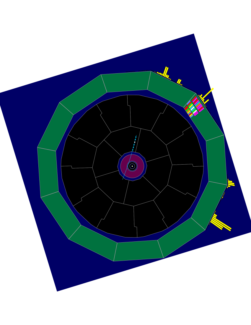
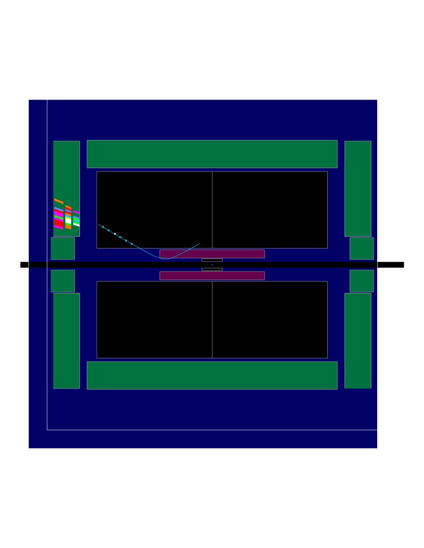
a). b).

Figure 5.7: An example of a track with $\matheuler{R}_{\tilde{l}}=1$ from signal Monte Carlo, viewed in (a) the $r\phi$ plane and (b) the $\rho z$ plane ($\rho$ is equal in magnitude to $r$, but with a sign that makes it negative for a certain half of the $\phi$ range which is chosen to make the event as clear as possible). Although the $\mathrm{d}_{0}$ of the track shows that the slepton reached a radius above at least one VDET layer before decaying, it did so at such a high $|\cos(\theta)|$ that it did not produce hits.

Chapter 6 Selections

This chapter describes the sets of cuts that are made on the variables calculated from the full event information that form the final discrimination between signal and background. There are two sets of six selections. The six selections of a given set are aimed at selecting with high efficiency events corresponding to each of the six possible final states ($\tilde{e}\tilde{e}$, $\tilde{\mu}\tilde{\mu}$, $\tilde{\tau}\tilde{\tau}$, $\tilde{e}\tilde{\mu}$, $\tilde{e}\tilde{\tau}$ and $\tilde{\mu}\tilde{\tau}$), while minimising the acceptance for background events. The difference between the two sets is only that the three most critical cuts are tuned under different conditions, such that one set gives optimal sensitivity in the case of low slepton decay-length, and the other in the case of high slepton decay-length. As such the two sets of six selections will be called the low and high decay-length optimisations. Both sets are applied independently to the real data and the Monte Carlo data, and so there are two sets of results described in Chapter 7. More details on the “hows and whys” of optimisation will be given in Section 6.4. The exact differences between the optimisations are given in Section 6.1.

Each selection is split into track and global cuts. Track cuts are cuts applied to variables that pertain to a given track within an event and are used to select good high-$\mathrm{d}_{0}$ tracks. Global cuts are cuts on variables that pertain to the event as a whole, such as the total energy or the number of charged tracks. The global cuts are quite loose in that they cause little (typically $<5\%$) signal rejection. The track cuts are more stringent and so the existence of one or more good high-$\mathrm{d}_{0}$ tracks is the most important property of a signal event. The relative importance of track and global cuts and a rationale for the general selection technique is discussed in Section 6.2.

6.1 Cuts common to all selections

Track cuts

All selections require at least one good high-$\mathrm{d}_{0}$ track ($N_{good}>0$ in the notation of Section 6.2). This section describes the track cuts that define what is meant by ‘good’.

The momentum, $\mathrm{d}_{0}$ and $\chi^{2}_{BS}$ (the $\chi^{2}$ of the track fit to the beam spot per degree of freedom) are the three variables whose associated cuts are tuned, and so are required to be greater than values which depend both on the channel and on the optimisation in question. Table 6.1 shows these values. A track is allowed to fail the $\mathrm{d}_{0}$ cut if its $\mathrm{z}_{0}$ is $>8\,\mathrm{cm}$. No other (global or track) cut depends on the optimisation, and so Table 6.1 completely summarises the difference between the low and high decay-length optimisations.

$\tilde{e}\tilde{e}$ $\tilde{\mu}\tilde{\mu}$ $\tilde{\tau}\tilde{\tau}$ $\tilde{e}\tilde{\mu}$ $\tilde{e}\tilde{\tau}$ $\tilde{\mu}\tilde{\tau}$ low $d_{\tilde{l}}$ 19.0 20.0 4.7 14.9 10.0 8.1 $p$ (GeV) high $d_{\tilde{l}}$ 19.8 18.6 6.1 20.0 8.5 4.3 low $d_{\tilde{l}}$ 0.17 0.50 0.13 0.09 0.24 0.5 $\mathrm{d}_{0}$ (cm) high $d_{\tilde{l}}$ 0.50 0.50 0.50 0.50 0.49 0.48 low $d_{\tilde{l}}$ 700 550 230 180 210 700 $\chi^{2}_{BS}$ high $d_{\tilde{l}}$ 680 690 700 700 590 610

Table 6.1: The cuts on track momentum ($p$), $\mathrm{d}_{0}$ and $\chi^{2}_{BS}$ for each channel under each optimisation. A track must have parameters greater than these values to be considered as a good high-$\mathrm{d}_{0}$ track in the corresponding selection.

The $\matheuler{R}_{\tilde{l}}$ of a track is required to be greater than 1, and it must have at least 4 assigned TPC hits and less than 3 bad TPC points (defined as a point where the track is missing a TPC hit for no observable reason – see Sections 5.5.1 and 5.5.2).

For the purpose of eliminating photon conversions the track has a variable called $r_{point}$. This is the radius at which the track’s circular $r\phi$ projection is pointing directly away from the origin. If the track has more than one hit at a radius below this then $r_{point}$ is set to zero. Tracks originating from photon conversions should be pointing away from the origin at the point where the conversion occurred, and should have no hits at lower radii. Thus tracks with $185\,\mathrm{cm}>r_{point}>4.5\,\mathrm{cm}$ are rejected. This is almost never satisfied by signal tracks, and is a very effective cut against photon conversion tracks since it does not rely on both the electron and the positron from the conversion being reconstructed.

To further reduce the background from nuclear interactions the distance of closest approach in three dimensions of each track to its nearest tagged nuclear interaction vertex (if there is one) is recorded and forms the variable $d_{NI}$. Tracks with $d_{NI}<5\,\mathrm{cm}$ are rejected. If the track is part of a multi-track vertex that failed both the nuclear interaction and $\tilde{\tau}\rightarrow\tau_{multi-prong}$ criteria, then it is rejected if the $\chi^{2}$ of the vertex is less than 100, and its maximum two-track angle is greater than 20^∘ or its kink angle is less than 20^∘. The latter two conditions reduce the probability of rejecting vertices that are due to slepton decay but which have not been identified as such.

To reduce the background from cosmic rays comparisons between the candidate tracks of an event are made. If two tracks do not have a reconstructed slepton-lepton vertex with a kink angle in $r\phi$ greater than 90^∘ at a radius greater than the 4th TPC pad row, and the difference between their $\mathrm{d}_{0}$’s is less than 10% of their average $\mathrm{d}_{0}$, then they are both rejected.

Tracks with $\matheuler{R}_{\tilde{l}}=5$ are required to have a slepton-lepton vertex radius less than that of the 20th TPC hit pad and a slepton momentum greater than $2\,\mathrm{GeV}$ (to further reduce background from ECAL splash-backs). Also, the track-fit $\chi^{2}$ (per degree of freedom) must be less than 4 (this is the fit of the helical track to the hits, not of the two tracks to the TPC-vertex).

Tighter cuts are made on tracks with $\matheuler{R}_{\tilde{l}}<5$. They are required to have at least one VDET hit with $r\phi$ information or $\mathrm{d}_{0}$$>2\,\mathrm{cm}$ or $\mathrm{z}_{0}$$>10\,\mathrm{cm}$. The track-fit $\chi^{2}$ is required to be less than 2.5. To reduce the cosmic ray background the momentum is required to be less then $150\,\mathrm{GeV}$. To reduce the background from low angle $\gamma\gamma$ events the $|\cos(\theta)|$ of the track is required to be less than 0.94, and if $\matheuler{R}_{\tilde{l}}=4$ the $|\cos(\theta)|$ of the slepton-lepton vertex is also required to be less than 0.94. Cuts are also made on the minimum possible $\tilde{l}\rightarrow l$ decay angle in two dimensions (the $r\phi$ projection), $\alpha_{min2}$, and in three dimensions, $\alpha_{min3}$. These are defined as the angle between the track and the line joining the track to the IP at the track’s innermost hit location. It is required that $\alpha_{min2}>1.5^{\circ}$ and $\alpha_{min3}>5^{\circ}$.

Global cuts

A certain degree of cosmic elimination is obtained by requiring that the event is not ‘class 3’. Classes are groups of basic cuts that an event is tested against after reconstruction. There are 25 in total and all events satisfy at least one of them. They are intended to speed up analyses by providing fast rejection of events that a user wishes to ignore. Class 3 is intended to flag cosmic rays passing through the VDET. It requires exactly two tracks with $\mathrm{d}_{0}$ $<$ 10 $\mathrm{cm}$, $\mathrm{z}_{0}$ $<$ 50 $\mathrm{cm}$, $|\cos(\theta)|<0.95$, p $>$ 10 $\mathrm{GeV}$ and with $>$ 9 TPC hits. It then requires that at least one of these must have a $\mathrm{d}_{0}$ $>$ 1 $\mathrm{cm}$ or a $\mathrm{z}_{0}$ $>$ 2 $\mathrm{cm}$, and that their directions differ by $>179^{\circ}$ in $\phi$, $<1^{\circ}$ in $\theta$, and their $\mathrm{d}_{0}$’s differ by $<0.5\,\mathrm{cm}$.

Further rejection of cosmic events is obtained by requiring $t_{0}$ $<$ 100 $\mathrm{ns}$, and that either the $\matheuler{R}_{\tilde{l}}$ of the best track is greater than 4 or that the total charged momentum from the IP is greater than $1\,\mathrm{GeV}$ or the cosine of the angle between the two highest momentum tracks that have TPC hits is $>-0.999$. If the $\matheuler{R}_{\tilde{l}}$ of the best track is less than 4 the additional constraint that the cosine of the angle between the two highest momentum tracks (regardless of hits) is also $>-0.999$.

Beam-gas events are rejected by requiring that the charged momentum from the IP be non-zero or that the ratio of transverse to longitudinal momentum from the IP be $>0.4$ (beam gas events are low angle and not centred in the detector).

6.2 Additional cuts for individual selections

In addition to the track cuts described in Section 6.1, tracks are also subject to an additional cut if they are to pass the $\tilde{e}\tilde{e}$, $\tilde{\mu}\tilde{\mu}$ or $\tilde{e}\tilde{\mu}$ selections. For the $\tilde{e}\tilde{e}$ selection only tracks with a non-zero probability of being an electron are accepted. The probability is calculated during reconstruction using calorimeter information. It is equal to zero if the track passes some very loose muon identification criteria. For the $\tilde{\mu}\tilde{\mu}$ selection only tracks with a muon probability (calculated during reconstruction using calorimeter and muon chamber information) greater than 0.2 are accepted. For the $\tilde{e}\tilde{\mu}$ selection a track must pass either of these conditions. No such cuts can be used in the channels involving staus since the high-$\mathrm{d}_{0}$ tracks can be electrons, muons or pions.

Events are also subject to additional selection-dependent global cuts. The global variables that are used are described in Table 6.2. Primed variables are calculated only using tracks and calorimeter deposits selected by the energy flow algorithm. For charged tracks this puts a cut of $2\,\mathrm{cm}$ on $\mathrm{d}_{0}$ and $10\,\mathrm{cm}$ on $\mathrm{z}_{0}$ since it is only intended for physics at the IP. The phrase ‘from the IP’ in Table 6.2 can be translated as ‘defined by energy flow’. Variables with an $\overrightarrow{\mathrm{arrow}}$ above them pertain to the ‘best’ track in the event. This is defined as the track with the highest value of $\matheuler{R}_{\tilde{l}}$. If there is more than one track with a $\matheuler{R}_{\tilde{l}}$ of 5 (the maximum) then the best is the one with the highest momentum. All energies and momenta are in units of  $\mathrm{GeV}$, all angles are in degrees.

Several variables refer to ‘hemispheres’ or ‘jets’. The event hemispheres are formed by finding the thrust axis of the event. This is the unit vector, $\mathbf{n}$, that minimises $\sum\mathbf{p}.\mathbf{n}$, where the sum is over all energy flow objects (charged tracks, photons and neutral hadrons) and $\mathbf{p}$ refers to the momentum 3-vector of a given object. Objects are then sorted into the hemispheres depending on which side of the axis they are closest to. The direction of a hemisphere is the direction of the sum of the 3-vectors of all its constituent objects. The jets are formed using the commonly used DURHAM algorithm [44]. The $y$-cut is chosen such that the event has exactly two jets, unless the event has only one object in which case jets are not defined. The direction of a jet is the direction of the sum of the 3-vectors of all its constituent objects.

Variable	Description
$N_{ch}$	Total number of reconstructed charged tracks
$N_{ch}^{\prime}$	Number of reconstructed charged tracks from the IP
$N_{e}$	Number of electrons
$\overrightarrow{P_{e}}$	Probability that the best track is an electron
$\overrightarrow{\matheuler{R}_{\tilde{l}}}$	The $\matheuler{R}_{\tilde{l}}$ of the best track
$c_{2ch}$	The cosine of the angle between the two highest momentum tracks
$N_{good}$	The number of tracks passing the track cuts (must be $\geq 1$)
$S_{2\beta}^{\prime}$	$\sqrt{1-0.5(\beta_{1}^{2}+\beta_{2}^{2})}$; where $\beta_{1}$ and $\beta_{2}$ are the boosts of the two hemispheres (one of which can be zero if the hemisphere contains no energy from the IP)
$\Phi_{aco}^{\prime}$	The acoplanarity of the jets (the angle between their $r\phi$ projections; defaults to 999 if the event cannot be forced into 2 jets)
$N_{TPC}$	The number of tracks that have TPC hits (tracks that have been tagged as originating from a non-SUSY secondary vertex are not included)
$N_{TPC}^{\prime}$	The number of tracks from the IP that have TPC hits
$\alpha_{hemi-z}^{\prime}$	The minimum angle between the plane of the hemisphere directions and the z-axis; defaults to 999 if one or more hemisphere contains no energy from the IP
$E_{tot}^{\prime}$	The total energy from the IP
$\overrightarrow{p}$	The momentum of the best track
$p_{t}^{\prime}$	The transverse momentum from the IP
$p_{z}^{\prime}$	The longitudinal momentum from the IP (unsigned)
$y_{23}^{\prime}$	The DURHAM algorithm $y$ cut for which the event goes from 2 to 3 jets
$c_{miss}^{\prime}$	The $|\cos(\theta)|$ of the momentum missing from the IP
$E_{beam}$	The LEP beam energy (constantly updated for real data by the LEP Energy Working group using 15 minute chunks of data, see [45])
$c_{thrust}^{\prime}$	The $|\cos(\theta)|$ of the thrust axis
$\overrightarrow{c}$	The $|\cos(\theta)|$ of the best track
$E_{12}^{\prime}$	The energy from the IP within 12 degrees of the beam axis (for Monte Carlo data this has an extra amount added taken randomly from a distribution determined from random triggers in order to simulate beam noise)
$N_{60\,\mathrm{GeV}}$	The number of tracks with $\mathrm{d}_{0}$$<0.5\,\mathrm{cm}$ and $\mathrm{z}_{0}$$<3\,\mathrm{cm}$ and a $\mathrm{d}E/\mathrm{d}x$ no less than 10 standard deviations below that which would be expected from a singly charged particle with a mass of $60\,\mathrm{GeV}$ (the approximate GMSB slepton mass limit)
$m_{tot}^{\prime}$	The invariant mass at the IP
$\alpha^{\prime}$	The acollinearity of the hemispheres (the angle between them; defaults to 999 if one or more hemisphere contains no energy from the IP)
$N_{\mu}$	The number of muons
$E_{tot}^{\pm}$	The total charged energy (tracks that have been tagged as originating from a non-SUSY secondary vertex are not included)
$p_{tot}^{\pm}$	The total charged momentum (tracks that have been tagged as originating from a non-SUSY secondary vertex are not included)

Table 6.2: The variables used in the selections and their definitions.

It may seem best to develop global cuts which, like the track cuts, tightly define the signal properties and so exclude background by the fact that it is non-signal-like. For example, it may seem sensible to require in the $\tilde{e}\tilde{e}$ selection that $4\leq N_{ch}\leq 6$ (since there should be four lepton tracks with possibly two slepton tracks) and $N_{e}=4$. But such simple cuts, while intuitive, cause significant losses in the signal efficiency. The reason for this is twofold. Firstly it is a matter of how large a loss of efficiency is considered significant. Because of the observable slepton lifetime the signal is extremely distinctive (see Figure 4.1), and so it should be possible to gain close to 100% efficiency with little background as long as the decay-length is of the right size. Thus while a cut which reduces the efficiency by (for example) 5% may be considered perfectly acceptable in most SUSY searches, here it is considered to have a significant detrimental impact and alternative cuts would be sought. The other reason is that the signal is simply not well defined by global variables. The slepton lifetime makes the usually indispensable tool of energy flow of very limited value, and interferes with the particle identification since the lepton tracks can be foreshortened and can cross the TPC wires and enter the calorimeters at unusually high angles to the radial direction. To go back to the earlier example, the cut $4\leq N_{ch}\leq 6$ causes an average loss of efficiency in excess of 10% over all the $\tilde{e}\tilde{e}$ Monte Carlo samples generated at 208 $\mathrm{GeV}$, and just the cut $N_{e}\geq 2$ causes more than a 10% loss in nearly half the samples. Thus to obtain the high efficiencies that must be achievable given the nature of the signal, the cuts on global variables must be set loose.

The strategy then was to focus the global cuts more on the properties of the background rather than that of the signal, and to ensure that they had virtually no effect on the signal efficiency for the whole ($m_{\chi}$, $m_{\tilde{l}}$, $d_{\tilde{l}}$) signal parameter space. Of course, in the case of slepton decay-length comparable to the $\mathrm{d}_{0}$-resolution of the detector, some cuts will have to have a severe impact on the efficiency. But these cuts should be those related to the one, well-defined and principal feature of the signal – the slepton decay-length, and so should be track cuts. Also, if the number of cuts with the potential to harm the efficiency are kept low, they can all be tuned by an optimisation process and the analysis as a whole will then be close to optimal. These are the cuts on track momentum, $\mathrm{d}_{0}$ and $\chi^{2}_{BS}$, which have already been described.

So the most important cuts in the analysis (those cuts which reject the large majority of the background) are the track cuts, and the global cuts serve only as a means of further discrimination in the case that an event has at least one good high-$\mathrm{d}_{0}$ track.

The additional global cuts are given in tabular form in Sections 6.2.1 to 6.2.6. The third column in each table indicates which Standard Model background the cut is intended to remove. If a cut is quite general in that it is effective against many backgrounds, then a ‘-’ is used. The cuts are grouped into numbered sets, where each set is intended to discriminate against the stated background. Ideally, every cut would have its associated plots of the distributions of the associated variable for signal and for background presented here, but given the number of cuts this is impractical, and so plots will only be shown for a few selected cuts.

6.2.1 Additional cuts for the $\tilde{e}\tilde{e}$ selection

The cuts are given in Table 6.3. The event is required to pass cut 1, and is only required to pass cut 2 if $N_{good}=1$ and $\overrightarrow{\matheuler{R}_{\tilde{l}}}=2$ (i.e. minimally signal-like – only one track passing the cuts with no evidence of the parent slepton). Cut 2 is an anti-$\tau\tau$ cut that discriminates against the high energy and (frequently) back-to-back nature of $\tau\tau$ events. It, or a slight variant of it, is used in every selection, and the distributions of the associated variables for the $\tilde{e}\tilde{e}$ channel and $\tau\tau$ background are shown in Figure 6.1 on page 6.1. $\tau\tau$ is a major background due to the $\tau$ lifetime which gives it a decay length of $\sim 5\,\mathrm{mm}$ at $E_{beam}\sim 100\,\mathrm{GeV}$, and the fact that the multi-prong decays are narrow which can lead to reconstruction difficulties as hits can be incorrectly assigned amongst the tracks from a single decay.

1	$20\!>\!N_{ch}\!>\!2$ $N_{ch}^{\prime}\!<\!7$ { $N_{e}\!>\!0$ or $\overrightarrow{P_{e}}\!>\!0.1999$ or $\overrightarrow{\matheuler{R}_{\tilde{l}}}\!>\!4$ }	$qq$
2	$0.99\!>\!c_{2ch}\!>\!-0.999$ { $S_{2\beta}^{\prime}\!>\!0.1$ or $\Phi_{aco}^{\prime}\!<\!174$ }	$\tau\tau$

Table 6.3: Additional cuts for the $\tilde{e}\tilde{e}$ selection

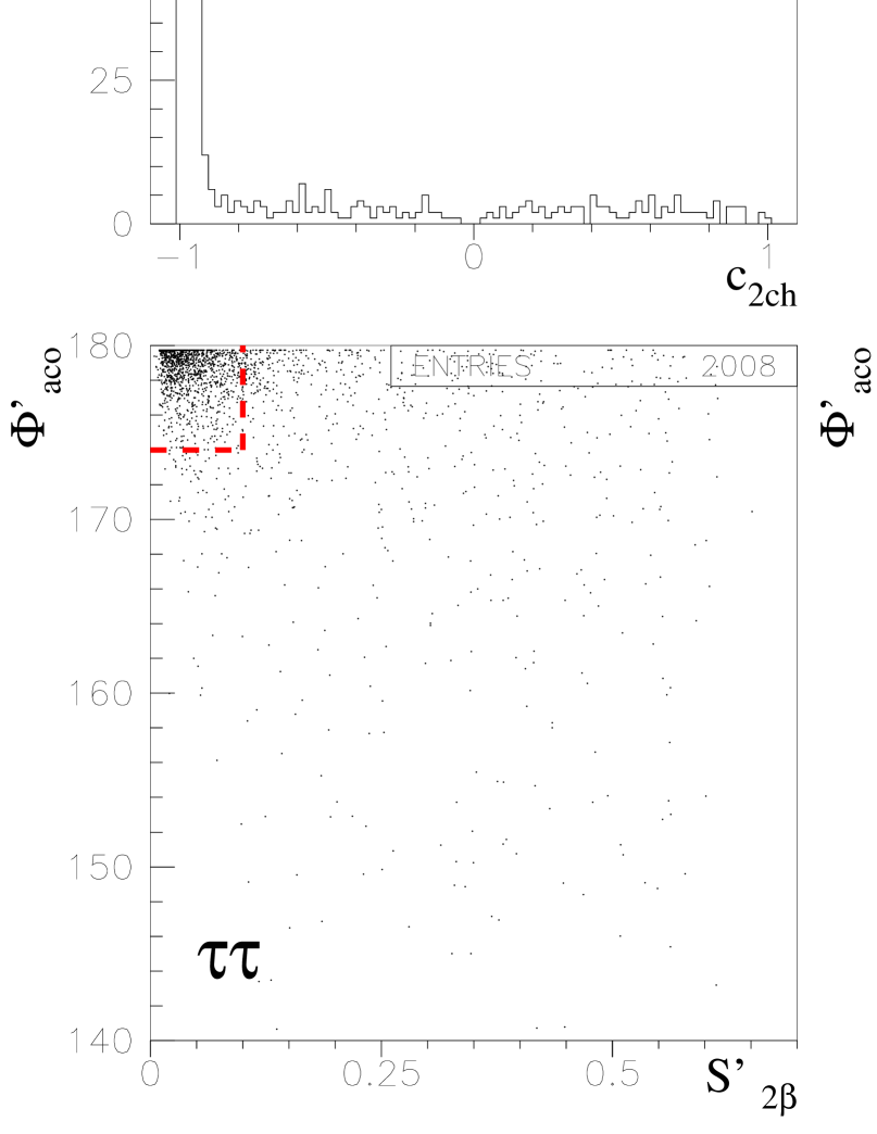
Figure 6.1: The distributions of $c_{2ch}$, $S_{2\beta}^{\prime}$ and $\Phi_{aco}^{\prime}$ for $\tau\tau$ and $\tilde{e}\tilde{e}$ Monte Carlo events at 189 $\mathrm{GeV}$. Top left is the full distribution of $c_{2ch}$ for $\tau\tau$ events. The two other plots on the same row show sub-ranges of the full distribution and the cut positions used in the anti-$\tau\tau$ cuts. The second and third rows show the same for $\tilde{e}\tilde{e}$ events with decay-lengths of 0.2 and 500 $\mathrm{cm}$ respectively. The fourth row shows scatter plots of $\Phi_{aco}^{\prime}$ versus $S_{2\beta}^{\prime}$ for the same samples. The rectangle in the top left of each plot shows the anti-$\tau\tau$ cut on these variables (events inside the rectangle fail the cut).

6.2.2 Additional cuts for the $\tilde{\mu}\tilde{\mu}$ selection

The cuts are given in Table 6.4. The event is required to pass cut 1. As with the $\tilde{e}\tilde{e}$ selection it is only required to pass cut 2 if $N_{good}=1$ and $\overrightarrow{\matheuler{R}_{\tilde{l}}}=2$.

1	$20\!>\!N_{ch}\!>\!2$ $N_{ch}^{\prime}\!<\!7$	-
2	$0.99\!>\!c_{2ch}\!>\!-0.999$ { $S_{2\beta}^{\prime}\!>\!0.1$ or $\Phi_{aco}^{\prime}\!<\!174$ }	$\tau\tau$

Table 6.4: Additional cuts for the $\tilde{\mu}\tilde{\mu}$ selection

6.2.3 Additional cuts for the $\tilde{\tau}\tilde{\tau}$ selection

The $\tilde{\tau}\tilde{\tau}$ selection is, as might be expected, the most complex of the six. The high-$\mathrm{d}_{0}$ tracks can be electrons, muons or pions and so no additional cuts can be made on the track properties. There are also difficulties with the global properties of the events. Whereas in a channel without staus there are only two invisible particles, in a $\tilde{\tau}\tilde{\tau}$ event the neutrinos from tau decay mean that there can be up to ten, leading to a much greater spread in the visible energy, and increased background from $\gamma\gamma$ events. The multi-prong decays also push up the multiplicity of the events which make $qq$ events more difficult to remove.

The cuts are given in Table 6.5. The event is required to fail cut 1. This is because cut 1 is intended to pick out $\gamma\gamma$ events from $\tilde{\tau}\tilde{\tau}$ events rather than the other way around. If $\overrightarrow{\matheuler{R}_{\tilde{l}}}=5$ then this is the only cut the event has to pass, although this is very rare in background events. If $\overrightarrow{\matheuler{R}_{\tilde{l}}}<5$ then the event also has to pass cuts 2 and 3 which are simple cuts on energy, mass, multiplicity and acollinearity. If there is no $\tilde{\tau}\rightarrow\tau_{multi-prong}$ candidate in the event it is also required to pass cuts 4 and 5, and to fail cut 6 (another pro-$\gamma\gamma$ cut). Under the hypothesis that the event is $\gamma\gamma$ and that only the electron/positron travelling in the direction of the missing momentum was deflected, then $p_{t}^{\prime}/(E_{beam}+p_{z}^{\prime})$ is the $\tan(\theta)$ of that electron/positron after deflection. Finally if $\overrightarrow{\matheuler{R}_{\tilde{l}}}<5$ and there is no $\tilde{\tau}\rightarrow\tau_{multi-prong}$ candidate and $\alpha_{hemi-z}^{\prime}<6$ and $N_{good}=1$ and $\overrightarrow{\matheuler{R}_{\tilde{l}}}\leq 3$ then the event is also required to pass cut 7, which is a variant of the anti-$\tau\tau$ cut used in the previous two selections.

Cut 4 is the most convoluted of the cuts. This is because it uses variables whose distributions for signal and background overlap significantly, but since $N_{TPC}$ and $\alpha_{hemi-z}^{\prime}$ are not correlated with each other or with $c_{thrust}^{\prime}$ and $c_{miss}^{\prime}$ (although $c_{thrust}^{\prime}$ and $c_{miss}^{\prime}$ are correlated), requiring events to pass only one of the cuts on these variables means the overall cut has significant impact on $qq$ events (approximately 90% fail) while leaving signal quite untouched (approximately 1% loss in efficiency). Figure 6.2 on page 6.2 shows the distributions of these variables and the cut values.

	$E_{tot}^{\prime}\!<\!40$ $p_{t}^{\prime}\!<\!8$ $p_{z}^{\prime}\!<\!20$ $N_{good}=1$ $\overrightarrow{p}\!<\!7$
1	$(y_{23}^{\prime}/0.1)^{2}+(1-c_{miss}^{\prime})^{2}+(E_{tot}^{\prime}/2E_{beam})^{2}\!<\!0.4$	$\gamma\gamma$
2	$14\!>\!N_{TPC}\!>\!2$ $N_{TPC}^{\prime}\!<\!11$	-
3	$(140E_{beam}/94.3)\!>\!E_{tot}^{\prime}\!>\!6$ $m_{tot}^{\prime}\!>\!7.7$ $\alpha^{\prime}\!<\!178$	$qq$
4	$E_{12}^{\prime}\!<\!25$ { $N_{TPC}\!<\!8$ or $\alpha_{hemi-z}^{\prime}\!>\!6$ or $(c_{thrust}^{\prime}\!<\!0.8$ and $c_{miss}^{\prime}\!<\!0.8)$ }	$qq$
5	$\overrightarrow{p}\!>\!5$ or $c_{miss}^{\prime}\!<\!0.95$	-
	$p_{t}^{\prime}/(E_{beam}+p_{z}^{\prime})\!<\!0.05$ $y_{23}^{\prime}\!<\!0.03$
6	$c_{miss}^{\prime}\!>\!0.8$ $c_{thrust}^{\prime}\!>\!0.8$ $N_{good}=1$ $\overrightarrow{c}\!>\!0.8$	$\gamma\gamma$
7	{ $0.99\!>\!c_{2ch}\!>\!-0.999$ or $\overrightarrow{\matheuler{R}_{\tilde{l}}}\!>\!2$ }{ $S_{2\beta}^{\prime}\!>\!0.2$ or $\Phi_{aco}^{\prime}\!<\!174$ }	$\tau\tau$

Table 6.5: Additional cuts for the $\tilde{\tau}\tilde{\tau}$ selection

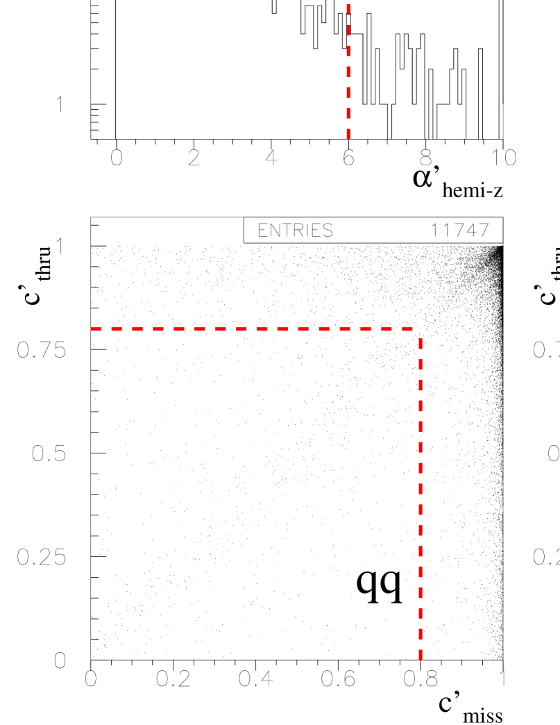
Figure 6.2: The distributions of $E_{12}^{\prime}$, $N_{TPC}$, $\alpha_{hemi-z}^{\prime}$ and of $c_{thrust}^{\prime}$ versus $c_{miss}^{\prime}$ for $qq$ and $\tilde{\tau}\tilde{\tau}$ Monte Carlo events at 189 $\mathrm{GeV}$. These are the variables used in cut 4 of the $\tilde{\tau}\tilde{\tau}$ selection. In the distributions of $\alpha_{hemi-z}^{\prime}$, values in excess of 10 have been placed in the last bin to retain the overall normalisation. The plots on the left are for $qq$ events, the centre plots for $\tilde{\tau}\tilde{\tau}$ events with a decay-length of 0.2 $\mathrm{cm}$, and the right plots for $\tilde{\tau}\tilde{\tau}$ events with a decay-length of 500 $\mathrm{cm}$. The cut values used in the $\tilde{\tau}\tilde{\tau}$ selection are shown as lines in the top three rows of histograms, and as rectangles in the bottom row (events outside the rectangle fail the cut).

6.2.4 Additional cuts for the $\tilde{e}\tilde{\mu}$ selection

The cuts are given in Table 6.6. The event must pass cut 1 and, if $N_{good}=1$ and $\overrightarrow{\matheuler{R}_{\tilde{l}}}=2$, cut 2 also.

1	$20\!>\!N_{ch}\!>\!2$ $N_{ch}^{\prime}\!<\!7$	$qq$
2	$0.99\!>\!c_{2ch}\!>\!-0.999$ { $S_{2\beta}^{\prime}\!>\!0.1$ or $\Phi_{aco}^{\prime}\!<\!174$ or $\alpha_{hemi-z}^{\prime}\!>\!6$ }	$\tau\tau$

Table 6.6: Additional cuts for the $\tilde{e}\tilde{\mu}$ selection

6.2.5 Additional cuts for the $\tilde{e}\tilde{\tau}$ selection

The cuts are given in Table 6.7. The event is required to pass cuts 1 and 2. Cut 3 is only applied if $\overrightarrow{\matheuler{R}_{\tilde{l}}}\leq 3$ since it can be damaging to signal efficiency when the slepton decay length is long. In particular, an upper limit on $E_{tot}^{\prime}$ is not applied if it looks like there is a fully reconstructed slepton in the detector ($N_{60\,\mathrm{GeV}}>0$ and $N_{TPC}<11$) since the slepton’s energy will be included by energy flow and so there may be no missing energy. Cut 4 is the standard $\tau\tau$ cut and is only applied if $N_{good}=1$ and $\overrightarrow{\matheuler{R}_{\tilde{l}}}=2$.

1	$N_{ch}^{\prime}\!<\!9$ $N_{ch}\!>\!2$ $N_{TPC}^{\prime}\!<\!10$ $N_{TPC}\!<\!12$	$qq$
2	$p_{t}^{\prime}/(E_{beam}+p_{z}^{\prime})\!>\!0.02$ { $m_{tot}^{\prime}\!>\!20$ or $p_{t}^{\prime}/(E_{beam}+p_{z}^{\prime})\!>\!0.1$ }	$\gamma\gamma$
	$E_{tot}^{\prime}\!>\!6$ $m_{tot}^{\prime}\!>\!7.7$ $\alpha^{\prime}\!<\!178$ $c_{miss}^{\prime}\!<\!0.999$
3	$E_{tot}^{\prime}\!<\!140E_{beam}/94.3$ or { $N_{60\,\mathrm{GeV}}\!>\!0$ and $N_{TPC}\!<\!11\,\}$	-
4	$0.99\!>\!c_{2ch}\!>\!-0.999$ { $S_{2\beta}^{\prime}\!>\!0.1$ or $\Phi_{aco}^{\prime}\!<\!174$ }	$\tau\tau$

Table 6.7: Additional cuts for the $\tilde{e}\tilde{\tau}$ selection

6.2.6 Additional cuts for the $\tilde{\mu}\tilde{\tau}$ selection

The cuts are given in Table 6.8. The event is required to pass cuts 1 and 2. Cuts 3 and 4 are the same as in the $\tilde{e}\tilde{\tau}$ selection and are only applied under the same circumstances. Cut 5 is an additional anti-$\gamma\gamma$ cut and is only applied if $N_{good}=1$.

1	$N_{ch}^{\prime}\!<\!9$ $N_{ch}\!>\!2$ $N_{TPC}^{\prime}\!<\!10$ $N_{TPC}\!<\!12$	$qq$
2	$N_{\mu}\!>\!0$ or $\overrightarrow{p}\!>\!10$	$\gamma\gamma$
	$E_{tot}^{\prime}\!>\!6$ $m_{tot}^{\prime}\!>\!7.7$ $\alpha^{\prime}\!<\!178$ $c_{miss}^{\prime}\!<\!0.999$
3	$E_{tot}^{\prime}\!<\!140E_{beam}/94.3$ or { $N_{60\,\mathrm{GeV}}\!>\!0$ and $N_{TPC}\!<\!11$ }	$\tau\tau$
4	$0.99\!>\!c_{2ch}\!>\!-0.999$ { $S_{2\beta}^{\prime}\!>\!0.1$ or $\Phi_{aco}^{\prime}\!<\!174$ }	$\tau\tau$
5	$E_{tot}^{\pm}\!>\!10$ { $c_{thrust}^{\prime}\!<\!0.8$ or $E_{tot}^{\pm}\!>\!30$ or $p_{tot}^{\pm}\!>\!25$ }	$\gamma\gamma$

Table 6.8: Additional cuts for the $\tilde{\mu}\tilde{\tau}$ selection

6.3 A note on the exclusivity of the selections

It should be noted that the selections are not mutually exclusive. That is to say, a single event can pass more than one of them. In fact, there is no combination of selections which an event, in principle, cannot satisfy. This is because the channels all give very similar final states, and so reliably disentangling one from another is practically impossible.

But exclusivity is very desirable amongst the selections of a search with more than one channel, since the results of the selections are then statistically independent, making any subsequent combination far simpler. Deliberate efforts could be made to ensure the selections are exclusive, but the method would have to be quite arbitrary, and would have a similarly arbitrary effect on the discovery/exclusion power of the search.

It would of course be possible simply to have a single selection aimed at selecting signal events from any channel. But in order to encompass all six channels without reproducing the same level of complexity of six individual selections, an all-inclusive selection would necessarily have to have a higher level of background acceptance.

The final states of the channels of the signal process fall mid-way between being different enough to allow exclusive selections, and being similar enough to allow a single selection, without harming the final result. Individual non-exclusive selections have been used then, and the complexity that follows is dealt with in the next chapter.

6.4 Optimisation

As has already been stated, the cuts on track momentum, $\mathrm{d}_{0}$ and $\chi^{2}_{BS}$ are the most critical of all the selection cuts. They cannot be set loose to encompass all the signal for any decay-length since they are very important in rejecting background, but if set too tight they will have a severe detrimental impact on the signal efficiency. They are therefore tuned to obtain the optimal cut values.

The definition of the optimal cut value is that which gives the lowest average expected 95% confidence level upper limit on the signal cross-section, $\overline{\sigma}_{95}$, that is the lowest average 95% confidence level cross-section limit that would be obtained over a large number of experiments in which the outcomes were as expected under the background-only hypothesis, as dictated by background Monte Carlo studies (the real data is not used). The methods for calculating the confidence level and $\overline{\sigma}_{95}$ will be given in Sections 7.3 and 7.5 respectively.

Ideally $\overline{\sigma}_{95}$ should be obtained as a function of all the cut values simultaneously. But since there are eighteen of these (three variables $\times$ six channels), and the method for calculating just a single cross-section limit is quite complex and CPU-intensive, this is impractical. Thus $\overline{\sigma}_{95}$ is obtained as a function of each cut value individually, first in the selection order $\tilde{e}\tilde{e}$, $\tilde{\mu}\tilde{\mu}$, $\tilde{\tau}\tilde{\tau}$, $\tilde{e}\tilde{\mu}$, $\tilde{e}\tilde{\tau}$, $\tilde{\mu}\tilde{\tau}$ for the cut on momentum, then the same for the cut on $\chi_{BS}^{2}$, and then for the cut on $\mathrm{d}_{0}$. At each stage the cut value that gave the smallest $\overline{\sigma}_{95}$ was identified and the cut set there. Cuts waiting to be tuned were set at sensible initial values.

A $\overline{\sigma}_{95}$ can only be calculated though, for a given signal hypothesis. That is, a given point in the ($m_{\chi}$, $m_{\tilde{l}}$, $d_{\tilde{l}}$) parameter space and a given set of values for the $\chi\rightarrow\tilde{e},\tilde{\mu},\tilde{\tau}$ branching ratios ($B_{\tilde{e},\tilde{\mu},\tilde{\tau}}$). Eight such signal hypotheses were used, corresponding to all permutations of high and low decay-length, high and low neutralino mass, and either slepton co-NLSP ($B_{\tilde{e},\tilde{\mu},\tilde{\tau}}=\frac{1}{3}$) or stau-NLSP ($B_{\tilde{e},\tilde{\mu}}=0$, $B_{\tilde{\tau}}=1$) branching ratios. The high and low decay-lengths used were 80 $\mathrm{cm}$ and 0.2 $\mathrm{cm}$, and the high and low neutralino masses were 95 $\mathrm{GeV}$ and 88 $\mathrm{GeV}$.

It was found however, that good sensitivity could be obtained under all the signal hypotheses using just the two optimisations obtained from the low decay-length, low neutralino mass, slepton co-NLSP combination, and the high-decay length, high neutralino mass, stau-NLSP combination. Since it was found that the optimised cut values were most strongly influenced by the choice of slepton decay-length, these optimisations were dubbed the low and high decay-length optimisations respectively, and the other optimisations were not used.

Chapter 7 Results and interpretation

7.1 Outcome

The number of background events expected to pass at least one selection, calculated from applying the selections to the background Monte Carlo samples, is shown in Table 7.1 for both optimisations (see previous chapter) along with the number of events observed in real data. The data is consistent with the background expectation, and so there is no evidence of supersymmetry. The numbers are broken down into seven bins by LEP energy – a re-binning with respect to Table 4.1. Since Monte Carlo background studies were only performed at energies of 189 and 208 $\mathrm{GeV}$, the expected numbers of background events for intermediate energies were gained by re-normalising the values at these two energies to the correct luminosity, and then linearly interpolating between them.

Energy $\matheuler{L}$ Low $d_{\tilde{l}}$ optimisation High $d_{\tilde{l}}$ optimisation (GeV) ($\,\mathrm{pb}^{-1}$) No. expected No. observed No. expected No. observed 188.6 174.2      1.4 $\pm$0.4 0    0.5 $\pm$0.3 1 191.6 28.9      0.2 $\pm$0.06 2    0.08 $\pm$0.04 1 195.5 79.9      0.7 $\pm$0.2 1    0.2 $\pm$0.1 1 199.5 87.1      0.7 $\pm$0.2 0    0.2 $\pm$0.1 0 201.6 44.4      0.4 $\pm$0.1 0    0.1 $\pm$0.06 0 205.0 79.9      0.7 $\pm$0.2 0    0.2 $\pm$0.1 0 206.7 133.7      1.2 $\pm$0.5 2    0.3 $\pm$0.2 1 Total      5.2 $\pm$1.4 5    1.5 $\pm$0.8 4

Table 7.1: A comparison of the expected number of events from background Monte Carlo studies with the number observed in data, broken down by LEP energy. $\matheuler{L}$ is the total integrated luminosity taken at each energy. The quoted errors are purely statistical in origin.

Since the selections for each channel are not mutually exclusive, a channel-by-channel breakdown of the number expected versus observed is not appropriate. Rather, the numbers (expected and observed) are broken down into those passing particular sets of selections. Since there are six selections there are ($2^{6}=$) 64 possible outcomes for the combination of selections that any event passes, including the complete set (passing all selections) and the null set (failing all selections, and therefore of no interest). The selection sets are numbered from 0 to 63 according to the convention

$$\mathtt{S}_{0\rightarrow 63}=32\,\delta_{\tilde{e}\tilde{e}}+16\,\delta_{\tilde{\mu}\tilde{\mu}}+8\,\delta_{\tilde{\tau}\tilde{\tau}}+4\,\delta_{\tilde{e}\tilde{\mu}}+2\,\delta_{\tilde{e}\tilde{\tau}}+\delta_{\tilde{\mu}\tilde{\tau}}\ ,$$

where $\delta_{chan}$ is 0 for events failing the respective channel’s selection, and 1 for events that pass. The expected versus observed number of events is shown broken down by selection set in Table 7.2. Only sets for which the expected background was non-zero, or for which a data event was observed are listed. No errors are quoted on the expected numbers of events in this table since, by breaking the numbers down by selection set, the events passing the selections become so thinly spread that each figure is typically based on no more than one event; and the procedure for calculating the (asymmetric) error on a weighted sum of Poisson variable estimators, when the estimators themselves are based on very few events, is extremely complex. Even without errors though, it is clear that the agreement for sets with a non-zero expected number of background events is good. Two events under each optimisation are observed however, with sets under which there were no events expected. Given that, overall, the number of background Monte Carlo events analysed was only around three times the number of events expected in the data set however, this does not constitute an incompatibility between real and background Monte Carlo data.

Selection Low $d_{\tilde{l}}$     Selection High $d_{\tilde{l}}$ set No. expected No. observed     set No. expected No. observed 8 3.0 2     2 0.6 1 2 0.6 0     5 0.4 0 5 0.4 0     3 0.2 1 3 0.2 0     11 0.2 0 10 0.2 1     39 0.2 0 12 0.2 0     8 0.0 1 11 0.2 0     9 0.0 1 36 0.2 0     39 0.2 0     44 0.2 0     4 0.0 1     14 0.0 1    

Table 7.2: A comparison of the number of expected events from background Monte Carlo studies with the number observed in data, broken down by selection set.

7.2 Efficiencies

Figures 7.1 to 7.3 show, for each channel, the probability of a signal event passing its own channel’s selection, and the probability of it passing at least one selection no matter which, as a function of decay length (estimated using the prescription described in Section 4.2.1) for both the low and high decay length optimisations. All plots are created from the Monte Carlo data generated at $\sqrt{s}=189\,\mathrm{GeV}$.

It can be seen that, in general, the selections other than that of the channel’s own selection add little to the total efficiency for a channel (i.e. if an event is not selected by its own channel’s selection, it is unlikely to be selected by another), as might be expected.

In each plot the different efficiency values at each decay length correspond to the different points in ($m_{\chi}$, $m_{\tilde{l}}$) space at which Monte Carlo data was generated (listed in Appendix A). All the points associated to the same ($m_{\chi}$, $m_{\tilde{l}}$) point are joined by a dotted line. This is for guidance only, it does not represent an interpolation. The dashed lines are formed by the straight line extrapolations from the two lowest and two highest decay length points. More will be said about these in Section 7.4. Note that there are many more mass points per decay length for the $\tilde{e}\tilde{e}$ channel since it was used as a test case to determine how many points in mass space would be needed for the subsequent Monte Carlo samples.

The very weak explicit dependence of the efficiencies on the neutralino and slepton mass is manifest. Most of the variation in the efficiency between the mass points at a given decay length can be accounted for by statistical fluctuation from a common value. In each plot there is one obvious exception however, most clearly at high decay length. In every plot the point with the highest efficiency at the highest decay length is the point with the least initial (i.e. before slepton decay) phase space open to the events. Specifically, for channels not involving staus it is the ($m_{\chi}$, $m_{\tilde{l}}$) point (94 $\mathrm{GeV}$, 93 $\mathrm{GeV}$); for channels that do involve a stau it is the point (94 $\mathrm{GeV}$, 91 $\mathrm{GeV}$). In both cases this is only a 0.5 $\mathrm{GeV}$ difference between the beam energy and the neutralino mass, and approximately a 1 $\mathrm{GeV}$ difference between the neutralino mass and the mass of the slepton plus that of the (heavier) lepton. The reason for the larger efficiency at high decay length for these points is that their decay length is greatly overestimated. The lack of phase space results in the slepton moving very slowly, so that its $\mathrm{d}E/\mathrm{d}x$ is very large. Thus the slepton is stopped by energy loss through ionisation almost as soon as it encounters any matter, and so typically does not penetrate the beam-pipe. Thus its decay length is effectively limited to $\sim 5\,\mathrm{cm}$. The efficiency does peak and then drop with decay length in a not too dissimilar way to the other points, but the drop-off at high decay length is not because the sleptons are increasingly escaping the tracking volume before decay. It is because in order to give such a slow-moving slepton such a large (estimated) decay length, the slepton lifetime has to be set very large (0.2 $\mu\mathrm{s}$ for a selectron at the stated mass point with $d_{\tilde{l}}=500\,\mathrm{cm}$). Once it is stopped in the beam-pipe it waits out the remainder of its lifetime before decaying. This can exceed the time period during which the ITC is active ($\sim 1\,\mu\mathrm{s}$), and so the resulting decay products (the high-$\mathrm{d}_{0}$ tracks) do not have ITC hits and so fail the quality criteria described in the previous chapters. This is increasingly likely with increasing estimated decay length and so causes the associated drop in efficiency, but still results in better efficiencies than the other points for the highest decay length.

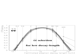
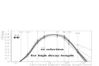
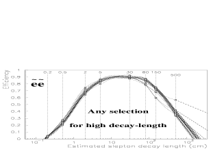
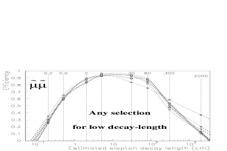
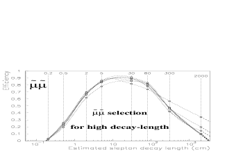
Figure 7.1: Efficiencies for the $\tilde{e}\tilde{e}$ and $\tilde{\mu}\tilde{\mu}$ channels as a function of estimated slepton decay length. The different curves correspond to different points in the ($m_{\chi}$, $m_{\tilde{l}}$) mass space.

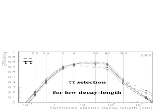
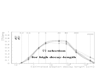
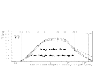
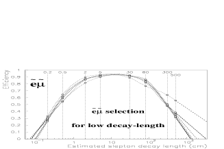
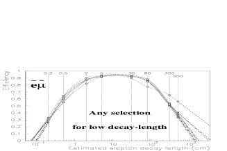
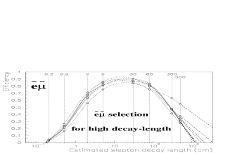
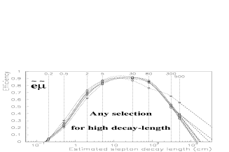
Figure 7.2: Efficiencies for the $\tilde{\tau}\tilde{\tau}$ and $\tilde{e}\tilde{\mu}$ channels as a function of estimated slepton decay length. The different curves correspond to different points in the ($m_{\chi}$, $m_{\tilde{l}}$) mass space.

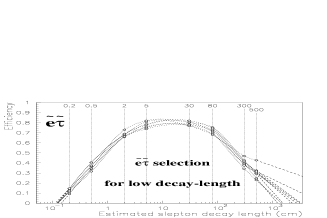
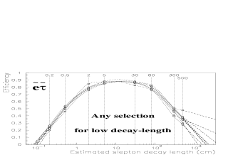
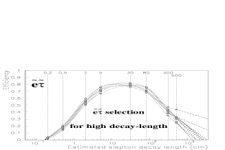
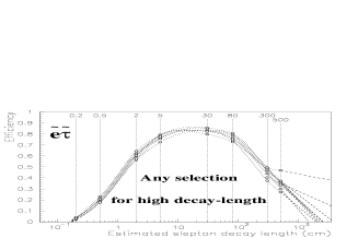
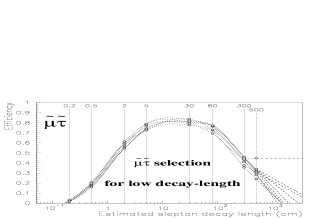
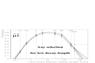
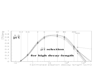
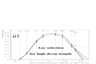
Figure 7.3: Efficiencies for the $\tilde{e}\tilde{\tau}$ and $\tilde{\mu}\tilde{\tau}$ channels as a function of estimated slepton decay length. The different curves correspond to different points in the ($m_{\chi}$, $m_{\tilde{l}}$) mass space.

The efficiencies for the $\sqrt{s}=208\,\mathrm{GeV}$ Monte Carlo data are not given since they are virtually identical when compared with the appropriate scaling (more will be said about this in Section 7.4). The slow-slepton effect resulting in the higher efficiencies for high decay lengths is not observed in the 208 $\mathrm{GeV}$ Monte Carlo data though, since the minimum $E_{beam}-m_{\chi}$ energy difference was limited to 1 $\mathrm{GeV}$. This shows that the effect is only confined to a very small corner of the mass space.

7.3 The confidence level

The ultimate goal of a search, in the absence of observing significant evidence for the signal, is to place the most stringent possible limits on the parameters of the underlying theory. Due to the statistical nature of particle physics, a search can never, with 100% certainty, rule out the hypothesised phenomenon. Only a ‘confidence level’, necessarily less than 100%, can be attached to the assertion that the phenomenon was not occurring. The confidence level is the probability that, if the hypothesised process were actually occurring, and if the experiment were done again in exactly the same way, a result more compatible with the hypothesis would be obtained. A high confidence level then indicates an experiment that is not compatible with the hypothesis, a low confidence level indicates one which is. The benchmark confidence level for ‘exclusion’ (disproof of the hypothesis) is 95%. At each point in the relevant parameter space the confidence level can be computed from the slepton and neutralino properties, and those points for which it is $\geq 95\%$ are said to be excluded. This section describes the way in which the confidence level is constructed. However, the method of construction used for this analysis is unusually complex for a SUSY search, and so there is first a discussion highlighting the motivation for this complexity.

The confidence level is computed from a ‘test statistic’, $t$, which itself is computed from the information yielded by the search. The test statistic should be a measure of how ‘signal-like’ (how compatible with the search hypothesis) the search outcome is. The higher its value, the more signal-like. Then if the expected probability distribution function of the test statistic under the signal hypothesis, $\rho(t)$, is known, the confidence level is given by

$$\mbox{CL}=1-\int\limits_{t_{min}}^{t_{meas}}\raisebox{28.45274pt}{}\!\rho(t)\ \mathrm{d}t\ ,$$

where $t_{min}$ is the minimum possible value of the test statistic, and $t_{meas}$ is the actual value from the search result. The definition of $t$ is, formally, completely free. Clearly it should be constructed such as to have good discriminating power between the signal and no-signal scenarios, but a bad choice only leads to a non-optimal confidence level (lower than the best possible). It does not make the confidence level wrong.

For the most optimal confidence level, $\rho(t)$ should take into account that some contribution to the value of $t$ is expected from background as well as from signal, and so should be the density of the test statistic under the signal-plus-background hypothesis. Any systematic errors in the simulation of the background however, then find their way into the confidence level. So the background contribution to $\rho(t)$ should be left out unless the background is well understood and its simulation is trusted. Since the background to this search comes from unconventional processes (principally particle interaction with the structure of the detector), the simulation of which have not been checked with the same rigour as more conventional sources, the background contribution to $\rho(t)$ is left out.

Typically with searches, as is the case with this search, the larger the number of observed events, the more signal-like the outcome. If there is no additional information associated with each event to discriminate signal from background, the only sensible choice for the test statistic is then just the number of observed events, $n_{obs}$. The confidence level is then given by

$$\mbox{CL}=1-\sum\limits_{n=0}^{n_{obs}}P_{n}=1-\sum\limits_{n=0}^{n_{obs}}\frac{e^{-n_{exp}}n_{exp}^{n}}{n!}\ ,$$

where $P_{n}$ is the (Poisson) probability of obtaining $n$ events as a search outcome, and $n_{exp}$ is the mean number of expected events under the signal (with no background) hypothesis.

In this way, a confidence level can be obtained for each channel by using

$$n_{obs}=\mbox{number of events passing channel's selection,}$$

$$n_{exp}=\matheuler{L}\,\sigma\,P_{chan}\,\varepsilon_{chan}\ ,$$

where $\matheuler{L}$ is the integrated luminosity, $\sigma$ is the neutralino cross-section, $P_{chan}$ is the probability that the neutralinos will decay such as to give this channel (given by the branching ratios), and $\varepsilon_{chan}$ is the efficiency with which events of this channel will be selected. For statistical reasons it cannot be said that the point is excluded if any one of these CLs is greater than 95%. The channel that appears most likely to exclude the point based on Monte Carlo studies only should be chosen, and if the CL of that channel (and that channel alone) is greater than 95% then the relevant point in parameter space is excluded.

This is clearly, however, a non-optimal approach. The information from five of the six channels is being thrown away. It should be possible, rather than to perform CL calculations for each channel individually, to calculate just one CL using all the data which would be greater than any one of the single-channel CLs. This cannot be calculated in a simple way from the single-channel CLs directly because the fact that the associated selections are not mutually exclusive means that the CLs are not statistically independent. A solution would be to use

$$n_{obs}=\mbox{number of events passing {any} selection,}$$

$$n_{exp}=\matheuler{L}\sigma\sum\limits_{chan=1}^{6}P_{chan}\varepsilon_{chan}\ .$$

But this is still non-optimal because it treats all observed events in an equal way. The number of expected signal events will be different between channels, and the number of expected background events will be different between the selections. Thus the contribution of an event to the value of the test statistic should be in some way representative of the discriminating power of the selection(s) it passes. In particular, in the case that the stau is significantly lighter than the selectron and smuon, and so effectively becomes the sole NLSP, it can be expected that including events that do not pass the $\tilde{\tau}\tilde{\tau}$ selection will only worsen the result.

A solution is to use the non-exclusivity of the selections as an extra source of information. The distribution of the signal efficiency amongst the 63 selection sets (disregarding the null set) is quite different from the equivalent distribution of the expected background. Thus the set of selections an event passes can be considered a discriminating variable that gives information on how signal-like it is. If the sets are numbered we have an integer variable, denoted $\mathtt{S}$, defined for each event with a value between 1 and 63. The test statistic can then be defined as the ratio of the probability of the search outcome under the signal-plus-background hypothesis to that of just the background hypothesis (i.e. a relative likelihood) taking into account the known numbers of signal and background events expected with each selection set:

$$t=\frac{L_{s+b}}{L_{b}}=\frac{\prod\limits_{\mathtt{S}}P(s_{\mathtt{S}}+b_{\mathtt{S}},n_{\mathtt{S}})}{\prod\limits_{\mathtt{S}}P(b_{\mathtt{S}},n_{\mathtt{S}})}\ .$$ (7.1)

$P(x,n)$ is the Poisson probability of observing $n$ events from an expected mean of $x$, $s_{\mathtt{S}}$ and $b_{\mathtt{S}}$ are the mean numbers of signal and background events expected to pass the set of selections, $\mathtt{S}$, respectively, and $n_{\mathtt{S}}$ is the observed number of events passing selection set $\mathtt{S}$. This test statistic now makes use of all the available information and copes naturally with variations in the number of expected signal events per channel and number of expected background events per selection.

A drawback is that $\rho(t)$ cannot be determined analytically now, only by a ‘toy’ Monte Carlo experiment. That is to say, using random numbers, a succession of hypothetical search results has to be generated in accordance with that which would be expected under the signal-only hypothesis. The corresponding test statistic can be calculated for each and a normalised histogram of these values built up to form $\rho(t)$.

The sorting of events by selection set now requires an associated decomposition of the efficiency. Thus we refer to the ‘total’ efficiency, defined as the probability of a signal event passing at least one selection, and the ‘partial’ efficiencies, defined as the 63 probabilities of a signal event passing each respective selection set. Then

$$s_{\mathtt{S}}=\matheuler{L}\sigma\sum_{chan}P_{chan}\epsilon_{\mathtt{S}\,chan}\ ,$$

and

$$\varepsilon_{chan}=\sum_{\mathtt{S}=1}^{63}\epsilon_{\mathtt{S}\,chan}\ \$$

where $\epsilon_{\mathtt{S}}$ denotes the partial efficiency associated with selection set $\mathtt{S}$, and $\varepsilon$ denotes the total efficiency.

So far the discussion has not incorporated the fact that the search detailed in this thesis spans a range of energies at which different amounts of data were taken, and for which the signal cross-sections and partial efficiencies will be different. This should also be built into the confidence level. If the data is split into a number of energy bins then the total test statistic is just the product of the single-energy test statistics calculated for each bin. Thus the generalisation of Eq. 7.1 to multiple energies is

$$t=\prod\limits_{e}t_{e}=\prod\limits_{e}\prod\limits_{\mathtt{S}}\frac{P(s_{\mathtt{S}\,e}+b_{\mathtt{S}\,e},n_{\mathtt{S}\,e})}{P(b_{\mathtt{S}\,e},n_{\mathtt{S}\,e})}\ ,$$ (7.2)

where $$e$$ denotes the energy bin and

$$s_{\mathtt{S}\,e}=\matheuler{L}_{e}\sigma_{e}\sum_{chan}P_{chan}\epsilon_{\mathtt{S}\,chan\,e}\ .$$

All the terms have the same basic definitions as before, but now a subscript $e$ means that value as defined at the centre-of-mass energy corresponding to energy bin $e$.

It is important to note that although numbers based on the background expectation are used to calculate the confidence level, any systematic error in these numbers can only, on average, reduce the confidence level. This goes back to a point mentioned at the start of this section – that the definition of the test statistic is completely free. A bad choice for the test statistic (or using incorrect numbers in the calculation of it) merely yields a less than optimal number. It is only in the calculation of the density of the test statistic under the signal hypothesis, $\rho(t)$, that systematic errors can cause a systematically inflated value, and the background expectation is not included in this.

For a more detailed discussion on the construction of test statistics, including the case of possible systematic errors in the background expectation, see [46].

7.4 Interpolation and extrapolation

This section describes the methods of interpolation and extrapolation employed to obtain the signal efficiencies for any given point in ($m_{\chi}$, $m_{\tilde{l}}$, $d_{\tilde{l}}$, $\sqrt{s}$) space. Such methods are required for the scans that will be described in Sections 7.5 and 7.6. The process is performed for each channel individually in stages. It is the partial efficiencies that are interpolated, and the total interpolated efficiency is their sum. Interpolation is first performed for four points in mass space to the correct mass point at decay lengths and $\sqrt{s}$’s above and below the desired values, then in decay length to form two points with the correct $d_{\tilde{l}}$, and then in $\sqrt{s}$ to arrive at the desired point. The following describes the procedure for a single channel.

Interpolation in mass space

For a given slepton decay length and $\sqrt{s}$, a method to gain the efficiencies for any point in ($m_{\chi}$,$m_{\tilde{l}}$) space was required. It was decided that a linear method was preferable for reasons of simplicity and transparency. The simplest method for linear interpolation in two dimensions is bilinear interpolation, but since the points in mass space do not form a rectangular grid, bilinear interpolation would lead to discontinuities in the (partial and total) efficiencies as a function of the masses. To get a continuous function the mass points have to be joined to make a tessellating set of polygons, and then an interpolation performed over each polygon. Since there is no obvious benefit from using polygons with a larger than minimal number of sides, only added complexity and less transparency, triangles were chosen as the polygons into which to split the plane. A commonly used and natural method for dividing a plane into triangles based on a set of points is called Delaunay triangulation (originally described in [47]), and this was the method used.

The Delaunay triangulation of a point-set is the collection of triangles which satisfy an “empty circle” property, i.e. the circle drawn through the vertices of any triangle does not enclose any other point from the set. As long as no circle can be drawn through four or more points then the collection is unique. If this is not the case then there are degenerate collections (i.e. more than one collection that satisfies the Delaunay criteria). This is the case with the sets of points in ($m_{\chi}$, $m_{\tilde{l}}$) space considered here, which do have subsets of four points (but never more) lying on common circles. Thus the degeneracy necessitates a choice for the diagonal down which the quadrilaterals defined by the co-circular points are to be split in order to form the triangles. The decision is always taken to split such quadrilaterals down the diagonal with the lowest average total efficiency in order to be conservative. The triangulation is thus performed for each channel, energy, decay length, and optimisation separately. It should be noted that no extrapolation is done in mass space – the efficiency is assumed to be zero outside the convex hull of the point-set.

Figure 7.4 shows examples of interpolated surfaces created by this method, and their associated Delaunay triangulations. Note that the range of the vertical scale has been limited to accentuate the variation of the surface. If viewed with a vertical scale from 0 to 1 both the surfaces appear almost flat. It is the fact that the efficiency is in general such a weak explicit function of the masses for a given decay length that allows the interpolation in mass space to be performed with so few points. Exceptions exist however, at high decay length. It can be seen from the efficiency plots of Section 7.2, that when the slepton mass is sufficiently close to the neutralino mass, and the neutralino mass is sufficiently close to the beam energy, the efficiency fails to fall as quickly with high and increasing decay length as for the other points in mass space. Thus the efficiency takes a sudden rise in the relevant corner of the mass space at the largest decay length. Since few points exist to map this rise an interpolation in this region would be dubious. In order to deal with this, the point with largest total efficiency at the maximum decay length has its total efficiency artificially reduced to that of the point with the second highest total efficiency, and the partial efficiencies are scaled accordingly. This was judged preferable to the large amount of extra Monte Carlo generation that would be needed to map this rise in such a small corner of the parameter space.

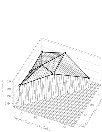
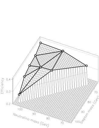
a).                                                            b).

Figure 7.4: The total efficiency as a function of neutralino mass and slepton mass for the $\tilde{e}\tilde{e}$ channel at 208 $\mathrm{GeV}$ under the high-$d_{\tilde{l}}$ optimisation at decay lengths of a). 30 $\mathrm{cm}$ and b). 500 $\mathrm{cm}$. The highlighted points on the surface show the points at which Monte Carlo data was generated. All other points on the surface are interpolated from these using the Delaunay triangulation which is shown superimposed.

Interpolation in decay length

As can be seen from the efficiency versus decay length plots of Section 7.2, a good method of interpolation in decay length would simply be to join the associated points with straight lines, and this is what is done. Although this is linear interpolation, it is linear with respect to $\log(d_{\tilde{l}})$ rather than $d_{\tilde{l}}$ itself. Unlike the treatment of mass space, extrapolation is used to extend the region of sensitivity to decay lengths beyond the maximum and minimum values at which Monte Carlo data was generated. This is performed by simply extending the straight lines joining the two highest and two lowest points in decay length down to the $x$-axis, as shown in the plots.

Extrapolation is possible because it is a mathematical certainty that the efficiency cannot drop completely to zero no matter how high or low the decay length. The efficiency can only approach zero asymptotically as the decay length falls to zero or extends to infinity. Thus the roughly straight lines that form the left and right sides of the efficiency ‘humps’ must level out at more extreme values. The extrapolations will thus give estimated efficiencies lower than the true efficiencies, and the extension of the lifetime range will be conservative. The beginning of this curve on the low decay length side can be seen in the plots for the high-$d_{\tilde{l}}$ optimisation.

There is an obvious problem with one ($m_{\chi}$, $m_{\tilde{l}}$) point in the $\tilde{\mu}\tilde{\tau}$ channel under the low decay length optimisation however, since the extrapolated line at high decay length does not descend to the $x$-axis. For one plot it is exactly horizontal, for the other it actually increases. But this is fixed by the reduction of the efficiency of this mass point at its highest decay length that is performed in order to make the interpolation in the mass plane valid (as described in the previous section). The plots of Section 7.2 are shown without this reduction. With the reduction the line drops to zero with the other mass points.

Interpolation in $\sqrt{s}$

The method of interpolation in $\sqrt{s}$ (the LEP centre of mass energy) is again linear, and is based on an empirical observation. The mass points chosen for the generation at 208 $\mathrm{GeV}$ were, for the most part, simply scaled from those chosen at 189 $\mathrm{GeV}$. That is to say, while the points occupy different positions in ($m_{\chi}$, $m_{\tilde{l}}$) space, they are at approximately the same positions in ($\frac{m_{\chi}}{E_{beam}}$, $\frac{m_{\tilde{l}}}{m_{\chi}}$) space (where $E_{beam}=\sqrt{s}/2$). It was observed that, for any given channel and decay length, the total and partial efficiencies of a point generated at 189 $\mathrm{GeV}$ were virtually identical to those of the point generated at 208 $\mathrm{GeV}$ which was closest in ($\frac{m_{\chi}}{E_{beam}}$, $\frac{m_{\tilde{l}}}{m_{\chi}}$) space with the same decay length. This simple scaling indicated that no further Monte Carlo data was required at intermediate energies – the efficiencies could be obtained for any intermediate energy by an appropriate interpolation.

To obtain the efficiencies at a given decay length $d_{\tilde{l}}$ and a given mass point ($m_{\chi}$, $m_{\tilde{l}}$) at LEP energy $E_{beam}$, the equivalent scaled masses ($\,\mathrm{m}_{\chi}^{\prime}$, $\,\mathrm{m}_{\tilde{l}}^{\prime}$) at 189 $\mathrm{GeV}$ and 208 $\mathrm{GeV}$ were found using the prescription:

$$\frac{\,\mathrm{m}_{\chi}}{E_{beam}}=\frac{\,\mathrm{m}_{\chi}^{\prime}}{E_{beam}^{\prime}}$$

and

$$\frac{\,\mathrm{m}_{\tilde{l}}+\overline{m}_{lepton}}{\,\mathrm{m}_{\chi}}=\frac{\,\mathrm{m}_{\tilde{l}}^{\prime}+\overline{m}_{lepton}}{\,\mathrm{m}_{\chi}^{\prime}}$$

where $E_{beam}^{\prime}$ is either 189 $\mathrm{GeV}$ or 208 $\mathrm{GeV}$ to obtain the respective equivalent masses, and $\overline{m}_{lepton}$ is the average of the masses of the two leptons involved in the channel (e.g. $(m_{\mu}+m_{\tau})/2$ for the $\tilde{\mu}\tilde{\tau}$ channel). The inclusion of the lepton masses in the scaling protects the $m_{\chi}-m_{\tilde{l}}$ mass difference from dropping below the mass of either of the leptons when scaling down in energy. Then the efficiencies can be obtained at the scaled mass points for the relevant decay length for both 189 and 208 $\mathrm{GeV}$, and then linearly interpolated to the correct energy, although the interpolation is not very important since the values will be very similar.

A method of quantifying the agreement of the partial and total efficiencies between 189 and 208 $\mathrm{GeV}$ was developed. For each point in ($m_{\chi}$, $m_{\tilde{l}}$, $d_{\tilde{l}}$) space at which 208 $\mathrm{GeV}$ Monte Carlo data was generated, the 189 $\mathrm{GeV}$ point closest in the ratio-space defined above with the same decay length was found. Note that although 360 points in total were generated at 208 $\mathrm{GeV}$, only 333 ($>90\%$) are directly comparable to 189 $\mathrm{GeV}$ points because the same decay lengths were not always generated at both energies. For each pair two $\chi^{2}$’s were calculated, one as a measure of the agreement of the total efficiencies and one as a measure of the agreement of the partial efficiencies without reference to their sum (it is thus a measure only of the relative sizes of the partial efficiencies, with any disagreement of the absolute sizes caused by a disagreement of the total efficiency removed). The former is defined as:

$$\chi^{2}=\sum_{i=1}^{2}\frac{(\overline{\varepsilon}-\varepsilon_{i})^{2}}{V_{i}}\ ,$$

where

$$\overline{\varepsilon}=\frac{\varepsilon_{1}V_{2}+\varepsilon_{2}V_{1}}{V_{1}+V_{2}}\ ;\hskip 28.45274pt\varepsilon_{i}=\frac{N_{i}}{500}\ ;\hskip 28.45274ptV_{i}=\frac{N_{i}}{500^{2}}\left(1-\frac{N_{i}}{500}\right)\ .$$

$\varepsilon_{i}$ is a total efficiency, $N_{i}$ is the number of events out of the total sample of 500 passing at least one selection, and the subscript $i$ refers to either 189 or 208 $\mathrm{GeV}$ Monte Carlo data depending on its value. The $\chi^{2}$ from the partial efficiencies was defined in a similar way for each selection set $\mathtt{S}$, and summed over, but now since the total number of events being considered is not fixed (events failing all selections, $500-N_{i}$ of them, are ignored) the errors are treated as Poisson as opposed to binomial:

$$\chi^{2}=\frac{1}{M}\sum_{\mathtt{S}=1}^{63}\sum_{i=1}^{2}\frac{(\overline{\eta}_{\mathtt{S}}-\eta_{\mathtt{S}i})^{2}}{V_{\mathtt{S}i}}\ ,$$

where

$$\overline{\eta}_{\mathtt{S}}=\frac{\eta_{\mathtt{S}1}V_{\mathtt{S}2}+\eta_{\mathtt{S}2}V_{\mathtt{S}1}}{V_{\mathtt{S}1}+V_{\mathtt{S}2}}\ ;\hskip 28.45274pt\eta_{\mathtt{S}i}=\frac{N_{\mathtt{S}i}}{N_{i}}\equiv\frac{\epsilon_{\mathtt{S}i}}{\varepsilon_{i}}\ ;\hskip 28.45274ptV_{\mathtt{S}i}=\frac{N_{\mathtt{S}i}}{N_{i}^{2}}\ .$$

$\epsilon_{\mathtt{S}i}$ is a partial efficiency corresponding to selection set $\mathtt{S}$, $N_{\mathtt{S}i}$ is the number of events out of the total sample passing selection set $\mathtt{S}$, and the other terms have the same definitions as for the previous $\chi^{2}$. $M$, the number of degrees of freedom to which the $\chi^{2}$ is normalised, is taken as the number of selection sets for which $N_{\mathtt{S}1}+N_{\mathtt{S}2}>0$, as opposed to the total of 63. This is because many of the selection sets have zero associated events at both energies and so do not contribute to the $\chi^{2}$. If they are included in the number of degrees of freedom the $\chi^{2}$ ends up artificially low.

a). Comparison of partial efficiencies, low $d_{\tilde{l}}$ optimisation. b). Comparison of partial efficiencies, high $d_{\tilde{l}}$ optimisation.

c). Comparison of total efficiencies, low $d_{\tilde{l}}$ optimisation. d). Comparison of total efficiencies, high $d_{\tilde{l}}$ optimisation.

Figure 7.5: The $\chi^{2}$ distributions resulting from compatibility tests between 189 and 208 $\mathrm{GeV}$ Monte Carlo data. In the two lower plots not all pairs of points gave a $\chi^{2}$ in the range shown. Such pairs have been placed in the last bin. Good agreement is shown amongst all the partial efficiencies, and most of the total efficiencies.

Both of these $\chi^{2}$’s are plotted in Figure 7.5 for the low and high $d_{\tilde{l}}$ optimisations. Good agreement between the relative sizes of the partial efficiencies is observed for all pairs of points. Good agreement between the total efficiencies is observed for most pairs of points, but some have $\chi^{2}$’s well in excess of 10 (seven are in excess of 100), and these have been placed in the last bins of the respective plots. All these pairs contain the 189 $\mathrm{GeV}$ low phase-space ‘problem’ points described in Section 7.2. It is not unsurprising that disagreement is observed here, since the same level of $E_{beam}-m_{\chi}$ degeneracy is not replicated in the 208 $\mathrm{GeV}$ Monte Carlo data, and the comparison is performed without the previously described efficiency reduction. The difference in the total efficiencies can thus be taken as a result of their slightly different positions in the mass-ratio space in a region where an anomalous effect is causing rapid change.

In summary, the signal efficiencies are almost imperceptibly weak functions of $\sqrt{s}$ for a given point in the stated mass-ratio space and a given $d_{\tilde{l}}$. Thus efficiencies can be reliably gained at all energies between 189 and 208 $\mathrm{GeV}$ by linear interpolation of the efficiencies calculated at these two energies.

7.5 Model independent cross-section limits

The cross-section limit is defined here as the 95% confidence level upper limit on the lightest neutralino production cross-section at a specific centre of mass energy for a given set of the relevant sparticle parameters (the neutralino mass and branching ratios, and slepton masses and lifetimes). Cross-section limits cannot be calculated analytically. A series of trial values are chosen and the confidence level is computed for each. Successive values are picked so as to converge on a computed confidence level of 95%. Once a confidence level sufficiently close to 95% is attained, the trial value can be taken as the cross-section limit.

Since the cross-section ($\sigma$) is a function of $\sqrt{s}$ however, and the search spans a range in $\sqrt{s}$, a different cross-section value must be used at each. These are related by the function, $\sigma(\sqrt{s})$, which defines the evolution of the cross-section with centre of mass energy. But the use of a specific model to gain $\sigma(\sqrt{s})$ will lead to limits that are not universally valid. This problem can be circumvented if the cross-section limit is calculated at (or above) the highest energy considered in the analysis, $\sqrt{s}_{max}$, and the cross-sections at lower $\sqrt{s}$ are obtained by a linear interpolation of the cross-section at the highest energy down to zero at threshold. Then the cross-section limits are valid as long as $\sigma=0$ and $\mathrm{d}^{2}\sigma/\mathrm{d}(\sqrt{s})^{2}$ is negative at $\sqrt{s}=2\,\mathrm{m}_{\chi}$ and there is no more than one stationary point in $\sigma(\sqrt{s})$ for $\sqrt{s}<\sqrt{s}_{max}$ (see Figure 7.6). Then if the real cross-section is larger than the cross-section limit at $\sqrt{s}_{max}$, it is also larger at all lower energies. This underestimation of the cross-section at lower energies for a given cross-section at $\sqrt{s}=\sqrt{s}_{max}$ leads to an underestimation in the confidence level, and thus an overestimation of the magnitude of the cross-section at $\sqrt{s}_{max}$ needed to give a confidence level of 95%. Thus the cross-section limit, quoted at $\sqrt{s}=\sqrt{s}_{max}$, will be conservative under these basic assumptions.

Figure 7.6: Schematic diagram of a hypothetical cross-section evolution with centre of mass energy and the interpolation used to evolve a cross-section at the highest energy down to lower energies. If the real cross-section is larger at the highest energy it is also higher at all lower energies.

Two scans over the ($m_{\chi}$, $m_{\tilde{l}}$, $\tau_{\tilde{l}}$) space were performed, with neutralino masses ranging from 68 to 103 $\mathrm{GeV}$, slepton masses ranging from 67 to $(m_{\chi}-1)$ $\mathrm{GeV}$ and values of $\log_{10}(\tau_{\tilde{l}})$ (where $\tau_{\tilde{l}}$ is measured in seconds) ranging from $-11.25$ to $-6.75$. The step size was 1 $\mathrm{GeV}$ in both the masses (i.e. integer values were used). The values of $\log_{10}(\tau_{\tilde{l}})$ were non-equidistant. For one scan the neutralino branching ratios to each slepton were set equal at $\frac{1}{3}$ (i.e. slepton co-NLSP scenario), for the other the neutralino was assumed to decay exclusively to stau plus tau (i.e. stau-NLSP scenario). The energy binning for the data was as shown in Table 7.1 (i.e. seven bins from 188.6 to 206.7 $\mathrm{GeV}$). At each point the partial efficiencies were calculated for each channel, energy and optimisation using the interpolation and extrapolation techniques described in Section 7.4. The total efficiencies were reduced by one standard deviation (and the partial efficiencies scaled accordingly) to be conservative. The background expectation values (the $b_{\mathtt{S}\,e}$ of Eq. 7.2) were linearly interpolated from the values determined from background Monte Carlo data at 189 and 208 $\mathrm{GeV}$. Note that in the case of an event being observed at an energy and with a selection set for which $b_{\mathtt{S}\,e}=0$, the value of the test statistic is infinite. This is clearly not sensible since the finite number of Monte Carlo background events analysed means that although no events may have been observed with a given selection set at a given energy, it does not necessarily mean that the mean expected number is non-zero. Thus, since approximately 10 times the number of events expected in data were analysed at 189 $\mathrm{GeV}$, and 100 times at 208 $\mathrm{GeV}$, a minimum value was placed on the $b_{\mathtt{S}\,e}$ of $(1-t)/10+t/100$, where $t=(\sqrt{s}_{e}-189)/(208-189)$ and $\sqrt{s}_{e}$ is the energy of the respective bin. A trial value for the cross-section limit at ($\sqrt{s}_{max}=$) 208 $\mathrm{GeV}$ was run down to the individual values at the seven bin energies. This gave all the information required to calculate a test statistic, as defined by Eq. 7.2, for any given experiment outcome.

Since there are two optimisations, there are two confidence levels. The confidence level chosen is the one which gives the higher average expected value under the background-only hypothesis (with no reference to the actual search outcomes). The exact procedure is as follows. Firstly the two test statistics for the actual observed outcomes under both optimisations are calculated. Then a series of 100 ‘toy’ Monte Carlo experiment outcomes are generated under the background-only hypothesis for each optimisation (i.e. using random numbers, 100 sets of hypothetical $n_{\mathtt{S}\,e}$ are generated in line with the values given by the Monte Carlo background expectation), and the test statistic is calculated for each. Then a sequence of toy outcomes are generated in the same way but under the signal-only hypothesis, and the test statistic is calculated for each. For each successive pair of signal outcomes the confidence levels for the two actual observed outcomes and the two sets of 100 toy background outcomes are updated. The confidence level for a given actual or toy background outcome after $N$ signal-only outcomes have been generated is given by

$$\mbox{CL}=1-\frac{n_{lower}}{N}\ ,$$

where $n_{lower}$ is the number of the toy signal outcomes which gave a test statistic less than or equal to the test statistic of the outcome under consideration. This obviously has an associated binomial error. Once the average of the 100 confidence levels under one optimisation becomes larger than that of the other’s to a good degree of statistical significance, the optimisation corresponding to the lower average is dropped and the process continues with just one optimisation. The upper and lower limits for the value of the confidence level corresponding to the one actual observed outcome still under consideration are taken as the upper and lower bounds of its 99.9% central confidence interval: CL_high and CL_low respectively. These are calculated for $N=30$, 100, 300, 1,000, 3,000, and 10,000. If CL_high is less than 95% then the point is considered un-excluded and the procedure stops. If CL_low is greater than 95% then the point is considered excluded and the procedure stops. If neither of these is true the procedure continues until the next value of $N$ at which they will be re-calculated. If $N$ reaches 10,000 with neither of these conditions being met then it is not known whether the confidence level is above or below 95%, only that it must be close. This is the requirement that must be satisfied for the trial value of the cross-section at 208 $\mathrm{GeV}$ to be considered the cross-section limit.

Figures 7.7 to 7.9 show the cross-section limit ($\sigma_{95}$) at $\sqrt{s}=208\,\mathrm{GeV}$ in units of nanobarns as a function of neutralino and slepton mass for each value of $\log_{10}(\tau_{\tilde{l}})$ considered. The left and right plots correspond to the slepton co-NLSP and stau-NLSP scenarios respectively. The contours show lines of constant cross-section limit. The $x$ ($m_{\chi}$) and $y$ ($m_{\tilde{l}}$) scales are identical (and so the line of slepton-neutralino degeneracy is the $45^{\circ}$ line joining the corners), and the cross-section limit is calculated at the mass-bin centres. The colour shading scheme is the same for all the plots, and the numbers on the keys to the right of each refer to values of $\log_{10}(\sigma_{95})$ (where $\sigma_{95}$ is in  $\mathrm{nb}$) and range from 0.924 ($\sigma_{95}=8.4\,\mathrm{nb}$) to 4.1 ($\sigma_{95}=12,590\,\mathrm{nb}$). In the lowest and highest lifetime plots for each scenario no limit exists beyond the outer contour (at $\sigma_{95}=10,000\,\mathrm{nb}$). The trial cross-section values were required to converge on $\sigma_{95}$ within a maximum number of iterations in order to ensure CPU-time was kept reasonable. In a few bins this did not occur, and so there are some spurious points where no limit is shown (appearing as isolated black squares). These are purely random occurrences and not the result of any physical effect.

The region of maximum sensitivity moves from bottom left to top right with increasing lifetime, since when the lifetime is short (long), low (high) neutralino and slepton masses are preferred to increase (reduce) the slepton decay length such that it is in the most sensitive region. Figure 7.10 shows the confidence level distributions for each scan. They are centred on 0.95 (95%) with a small spread, as expected. For comparison with the quoted limits, a perfect search (100% efficiency and zero observed events) would yield a limit of

$$\sigma_{95}=-\ln(1-0.95)\frac{(208-2m_{\chi})}{\sum\limits_{e}\matheuler{L}_{e}(\sqrt{s}_{e}-2m_{\chi})}$$

where the 0.95 is the confidence level, and elements in the sum over energy bins for which $\sqrt{s}_{e}<2m_{\chi}$ are ignored. The $m_{\chi}$ dependence comes from the assumed linear evolution of the cross-section with $\sqrt{s}$. This function is plotted in Figure 7.11 together with a comparison with the obtained limit at $\log\tau_{\tilde{l}}=-8.75$ under the co-NLSP scenario.

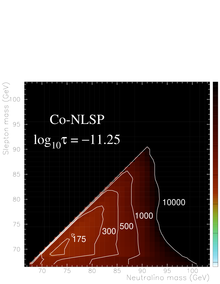
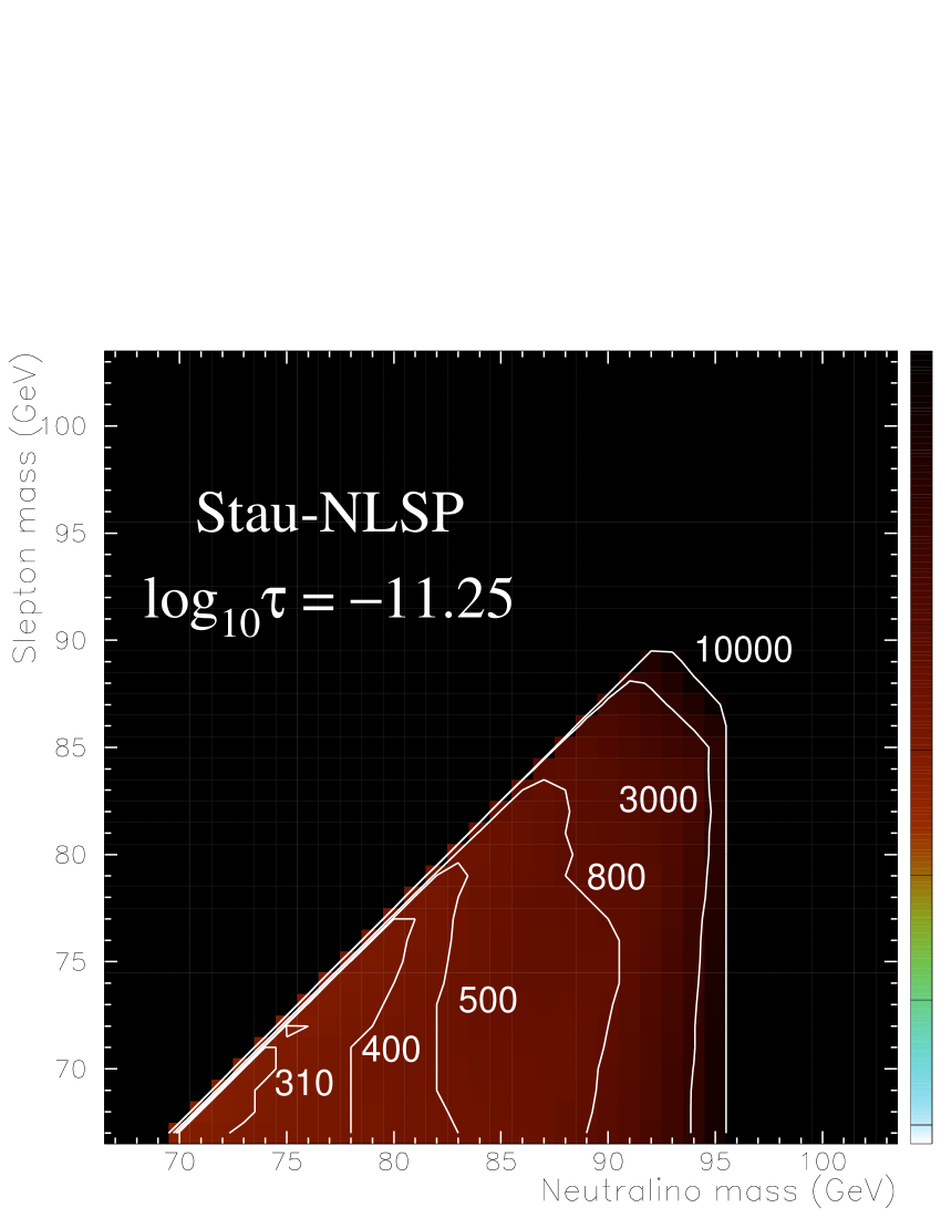
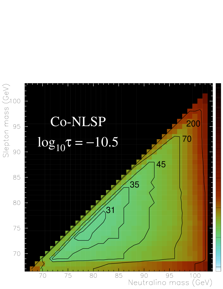
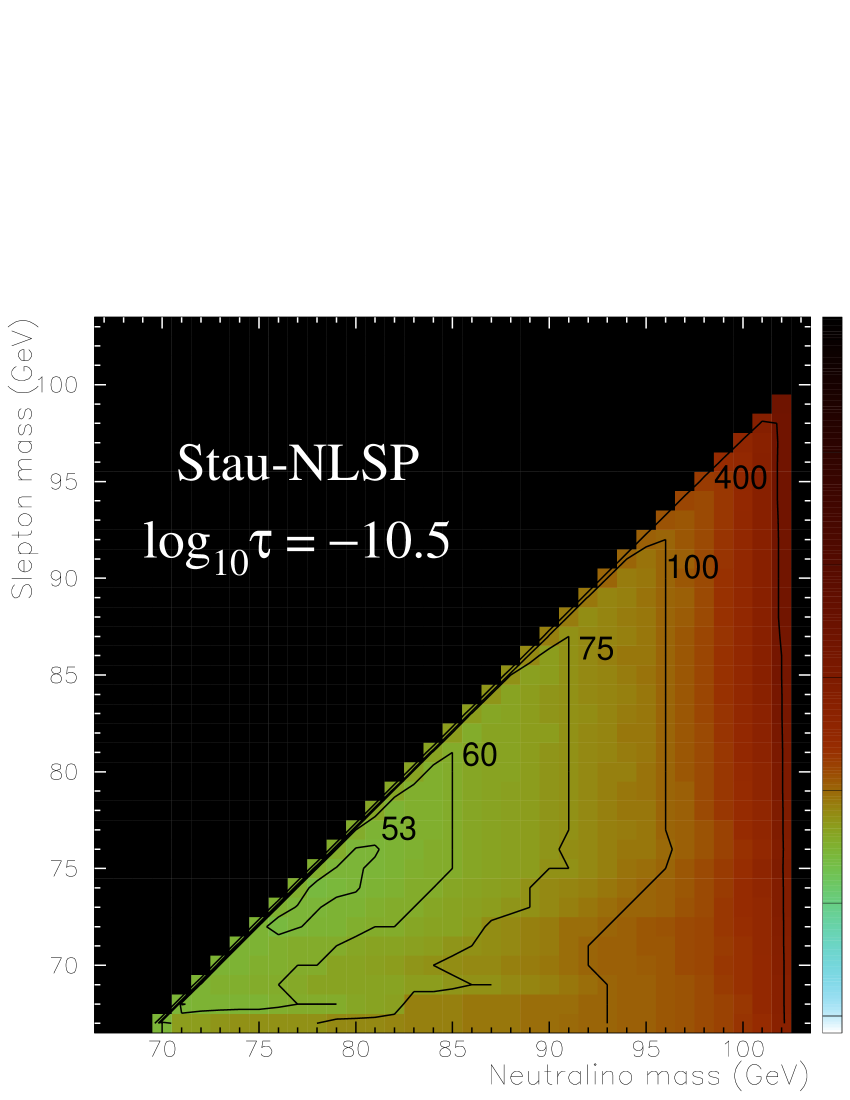
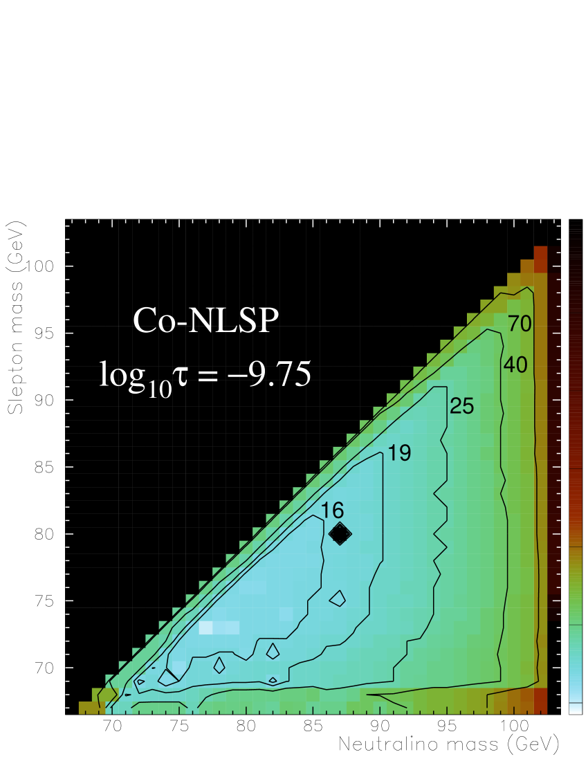
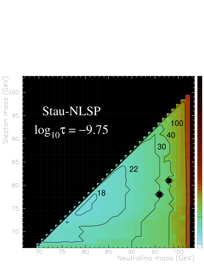
Figure 7.7: Model independent limits on the neutralino production cross-section at a LEP energy of 208 $\mathrm{GeV}$ as a function of neutralino and slepton mass. The limits are at 95% confidence level and in units of nanobarns. ‘Co-NLSP’ means the neutralino was assumed to decay to the three sleptons with equal branching ratios of $\frac{1}{3}$. ‘Stau-NLSP’ means the neutralino was assumed to decay exclusively to the stau. The slepton lifetime is the ‘$\tau$’ in $\log_{10}\tau$ and is measured in seconds.

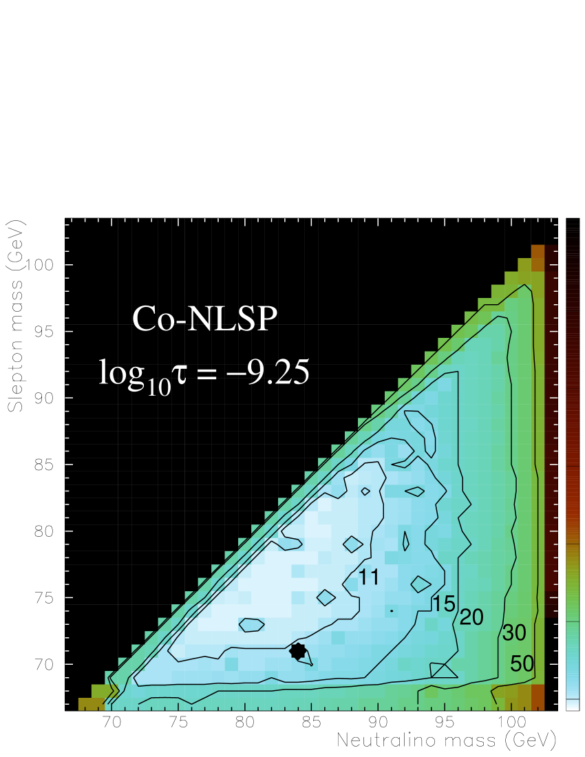
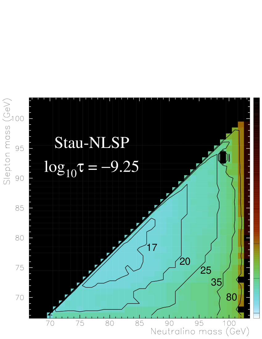
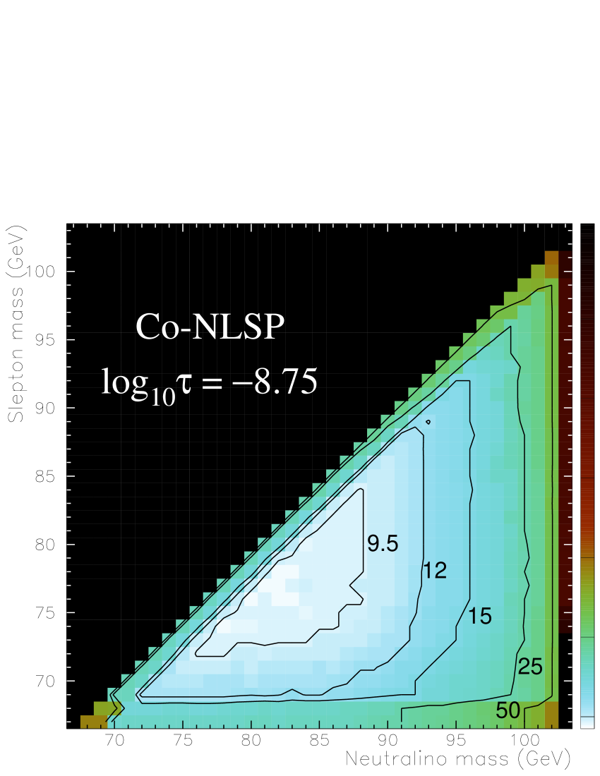
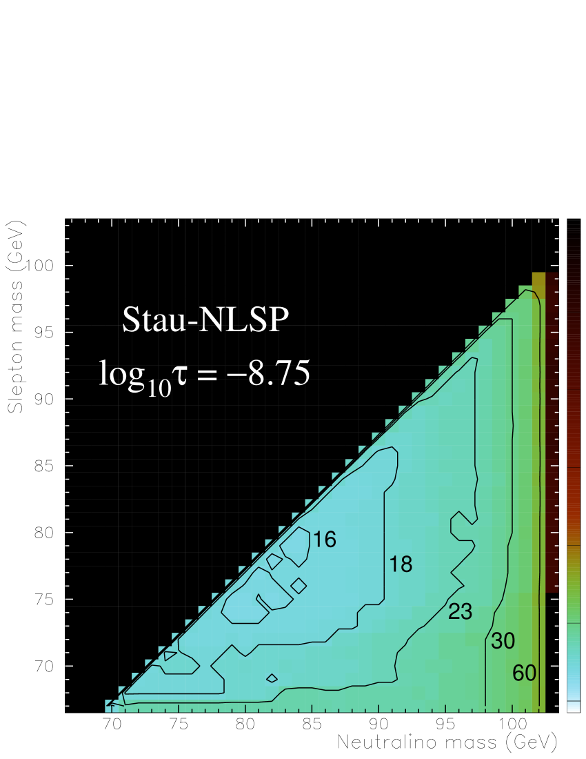
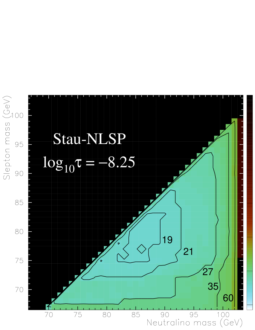
Figure 7.8: Model independent limits on the neutralino production cross-section at a LEP energy of 208 $\mathrm{GeV}$ as a function of neutralino and slepton mass. Limits are given at 95% confidence level in units of nanobarns for the co-NLSP and stau-NLSP scenarios and a range of slepton lifetimes.

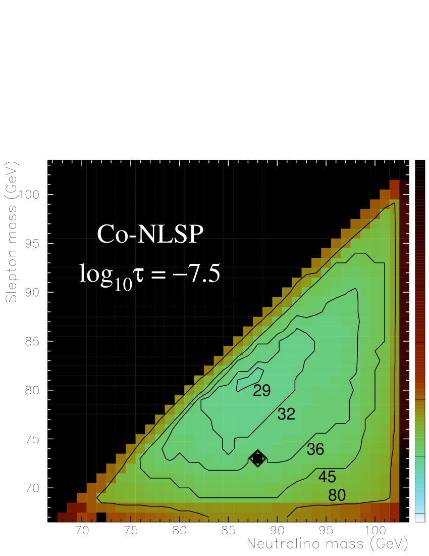
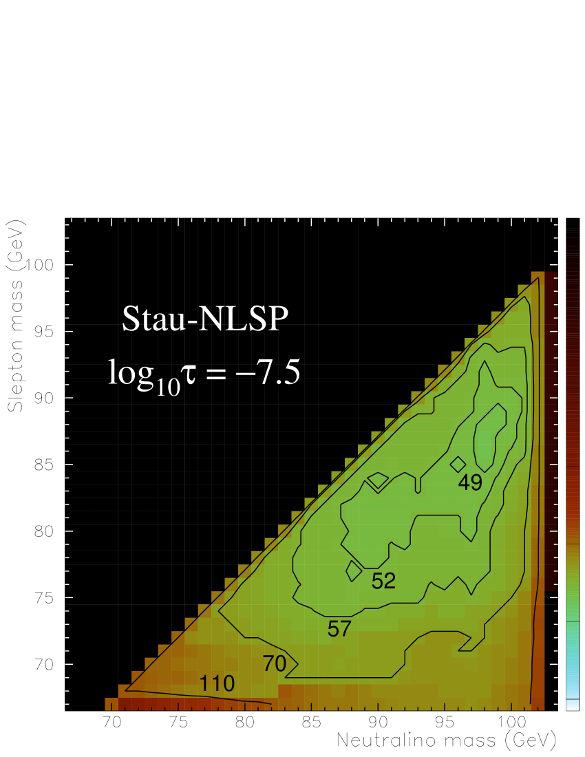
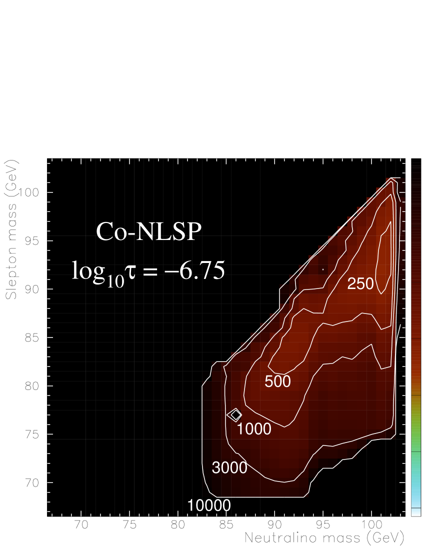
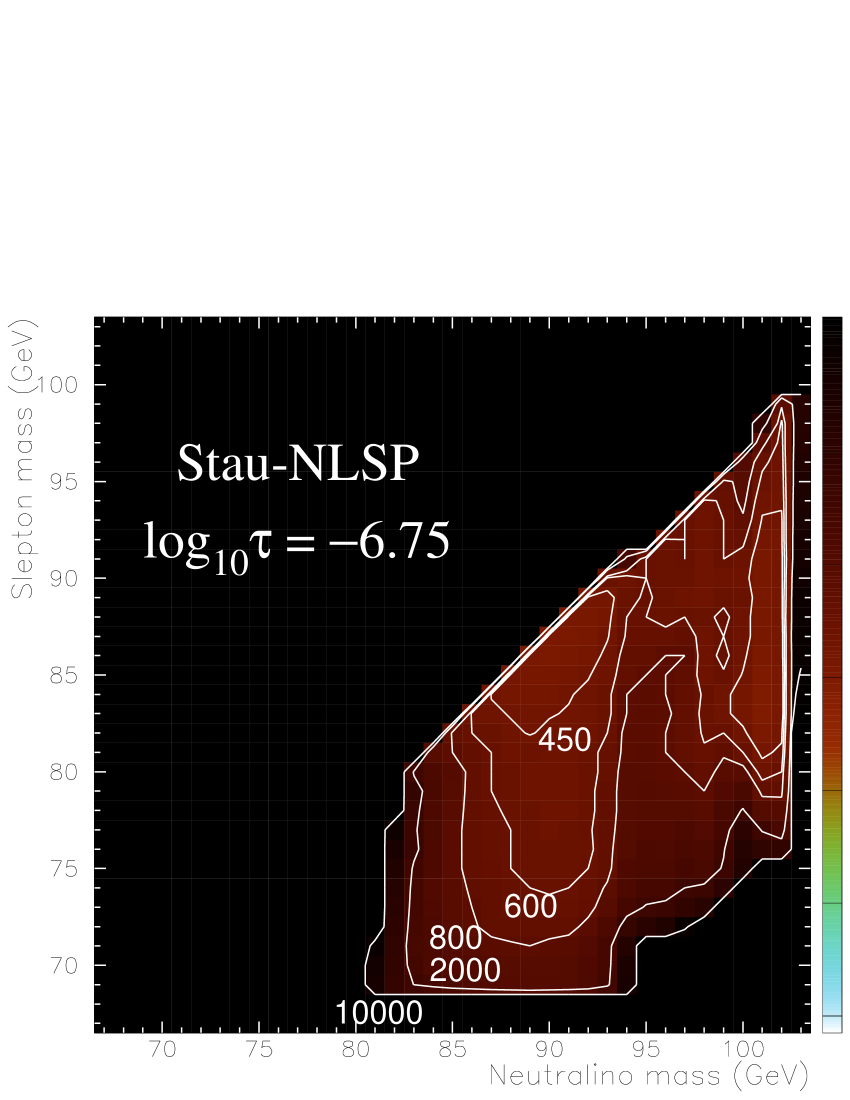
Figure 7.9: Model independent limits on the neutralino production cross-section at a LEP energy of 208 $\mathrm{GeV}$ as a function of neutralino and slepton mass. Limits are given at 95% confidence level in units of nanobarns for the co-NLSP and stau-NLSP scenarios and a range of slepton lifetimes.

Figure 7.10: The distributions of the confidence levels by which the cross-section limits are excluded. They are centred on 0.95 with a small spread.

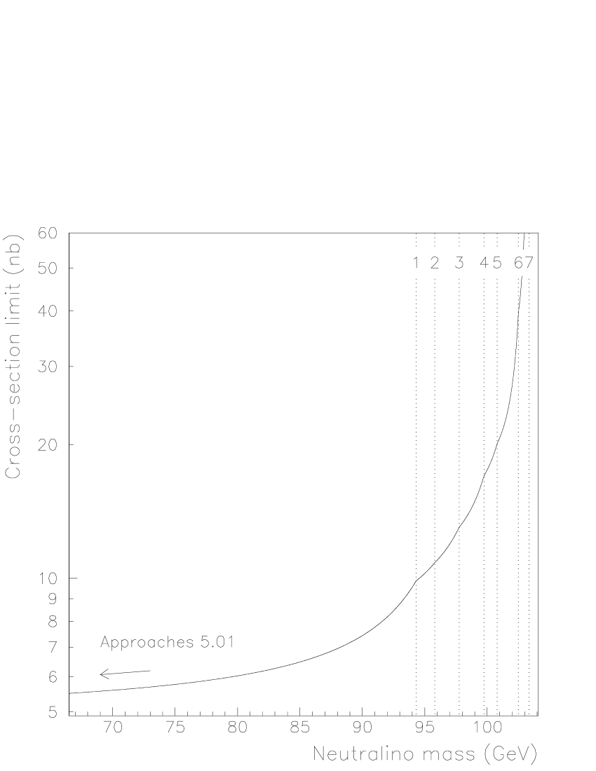
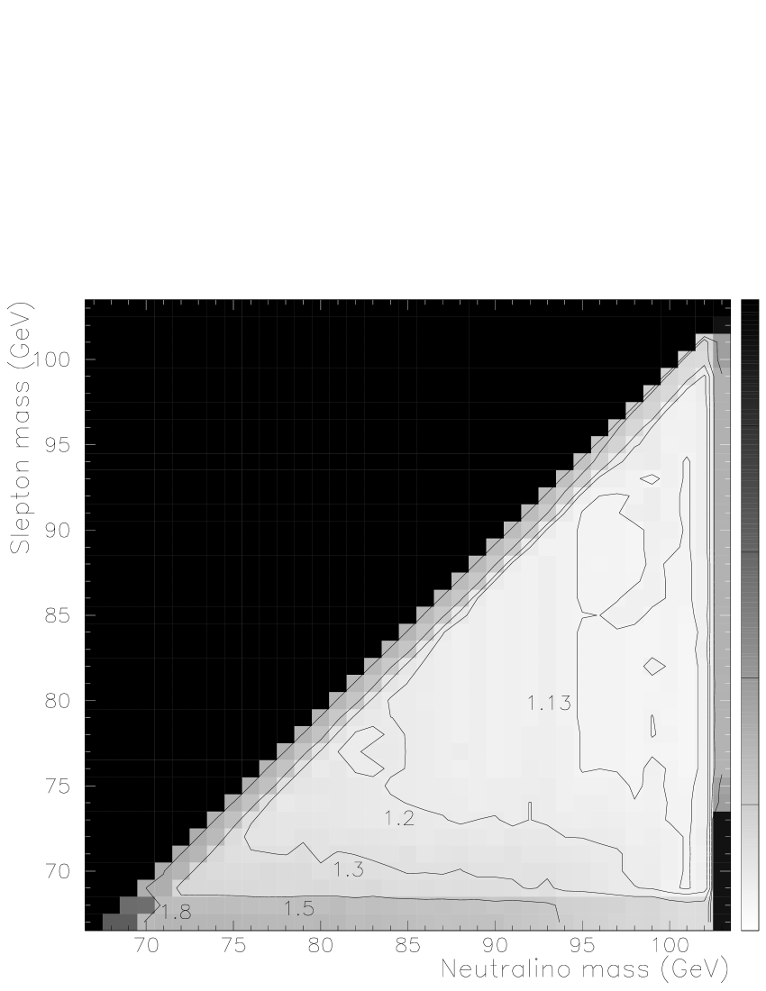
a).b).

Figure 7.11: a). The cross-section limit at 208 $\mathrm{GeV}$, as a function of $m_{\chi}$, that would result from a search with 100% efficiency and which gave zero observed events. The limit increases smoothly with $m_{\chi}$ because, for a given cross-section at 208 $\mathrm{GeV}$, a higher neutralino mass causes a lower cross-section at the lower energies (according to the linear evolution scheme described earlier). The gradient has discontinuities however, corresponding to the neutralino mass exceeding the beam energies of successive energy bins. b). A plot of the ratio of the limit for the co-NLSP scenario with a $\log\tau_{\tilde{l}}=-8.75$ to the ideal limit shown in the plot on the left. It shows that the limit obtained is close to the theoretical minimum.

7.6 Model specific parameter space exclusion

A scan over the parameter space of the model described in [20] was performed by Aran Garcia-Bellido in order to translate the results of all the ALEPH GMSB searches into excluded regions of the model’s parameter space. This was an update of the scan described in [16] using the new highest energy LEP data and including the analysis described in this thesis. The scan ranges for the parameters (which are described in Section 2.6.4) and the number of points used in each are given in Table 7.3. The five values for the upper limit on $\Lambda$ correspond to increasing values of $\mathrm{N5}$, i.e. for $\mathrm{N5}=1$ the upper limit on $\Lambda$ is 75 $\mathrm{TeV}$, for $\mathrm{N5}=2$ the upper limit is 60 $\mathrm{TeV}$, etc. At each point the ISAJET 7.51 program [48] was used to calculate the sparticle masses, branching ratios and lifetimes, together with their production cross-sections at the seven LEP energies given in Table 7.1.

Parameter Lower limit Upper limit No. of points $\mathrm{M_{mess}}$ $10^{4}\,\mathrm{GeV}$ $10^{12}\,\mathrm{GeV}$ 5 $\mathrm{M_{\tilde{G}}}$ $10^{-9.5}\,\mathrm{GeV}$ $10^{-4}\,\mathrm{GeV}$ 12 $\Lambda$ $2\,\mathrm{TeV}$ $75,60,45,45,45\,\mathrm{TeV}$ 151 $\tan\beta$ $1.5$ $40$ 9 $\mathrm{N5}$ $1$ $5$ 5 $\mathrm{sign(\mu)}$ $-$ $+$ 2

Table 7.3: The ranges for the scan parameters and the number of points in each. 815,400 points were considered in total.

These were then passed to the same routine that calculated the confidence level for the cross-section limit scan, and the same method was used for judging whether the confidence level was greater than, less than, or not distinguishable from 95%. Points with a confidence level greater than 95% were considered excluded, points with a confidence level less than, or indistinguishable from 95% were considered unexcluded.

One problem arose in this scan which did not arise in the cross-section limit scan however. In the cross-section limit scan only the case of perfect slepton degeneracy, and the case of a stau so much lighter than the selectron and smuon it was effectively the sole NLSP were considered. In this scan, points in-between these two extremes exist, where the stau is significantly lighter but the neutralino branching ratios to the selectron and smuon are still quite significant. This does not pose a problem for the $\tilde{e}\tilde{e}$, $\tilde{\mu}\tilde{\mu}$, $\tilde{\tau}\tilde{\tau}$ and $\tilde{e}\tilde{\mu}$ channels since the two sleptons involved in each channel are still degenerate with each other. But events in the $\tilde{e}\tilde{\tau}$ and $\tilde{\mu}\tilde{\tau}$ channel will involve sleptons of different properties in the same event – a case for which signal Monte Carlo data has not been generated. However, since the efficiencies (partial and total) depend almost solely on the slepton decay length, it can be expected that the true efficiencies will lie somewhere between those calculated based on both sleptons having the stau’s properties, and those based on both having the other slepton’s properties. Although it cannot be expected that the true efficiencies can be obtained by any kind of simple interpolation between the two, it can be expected that the true confidence level will lie between the confidence levels calculated assuming both sleptons have the one set of properties and both having the other. So two confidence level calculations are run in parallel for both optimisations, and the lowest is chosen as the real confidence level to be conservative.

Significant regions of excluded parameter space in the ($m_{\chi}$, $m_{\tilde{\tau}}$) plane were only found for four of the twelve gravitino masses used in the scan, and these regions are shown in Figure 7.12. The sudden rise in the lower edges around $m_{\chi}\sim 90\,\mathrm{GeV}$ corresponds to the threshold for neutralino production beginning to exceed the energies at which data was taken. The positions of the lower edges of the regions for $\mathrm{M_{\tilde{G}}}=\!10^{-8}$, $10^{-7.5}$ and $10^{-7}$ $\mathrm{GeV}$ are predominantly defined by the lowest slepton mass for which Monte Carlo data was generated rather than any physical effect. For $\mathrm{M_{\tilde{G}}}=\!10^{-6.5}$ $\mathrm{GeV}$ the lower edge is higher. This is because the slepton lifetime is proportional to ($\mathrm{M_{\tilde{G}}}^{2}/m_{\tilde{l}}^{5}$). So for a high gravitino mass and decreasing slepton mass the slepton decay length can rise beyond the maximum value for which there is sensitivity before the slepton mass drops below the minimum defined by Monte Carlo data. A similar effect accounts for the fact that the right hand edge of the $\mathrm{M_{\tilde{G}}}=\!10^{-8}$ $\mathrm{GeV}$ region is at a lower value of $m_{\chi}$ than for the other regions. Here the slepton lifetime is short, and a high neutralino mass exacerbates this to produce a decay length below the minimum value for which there is sensitivity.

Figure 7.12: Excluded regions of ($m_{\chi}$, $\,\mathrm{m}_{\tilde{\tau}}$) space for four different gravitino masses.

7.7 The results in a wider context

The analysis described in this thesis was incorporated in an update of the common interpretation of all ALEPH GMSB work in [49]. This includes a description of a scan essentially identical to that described in Section 7.6, and contains plots similar to those in Figure 7.12 but showing the regions excluded by every search. The search described in this thesis did not exclude any significant amount of parameter space that the search for direct slepton pair production over the same energy range ([50]) did not, since although the neutralino cross-section was often higher, the slepton cross-section was never so low that points could not be excluded by the slepton pair-production search when they could be by this search. The search for pair-produced sleptons is also not limited by the neutralino mass and so covers a wider range of the parameter space. This search then serves to confirm the exclusion of the relevant region of parameter space under the model considered, but still could prove independently useful should models be hypothesised in the future which predict a greater disparity between the neutralino and slepton cross-sections. It also brings the overall ALEPH GMSB search effort close to complete.

The current ALEPH limits are given in [49] as:

In the neutralino-NLSP scenario:
99 $\mathrm{GeV}$	on $m_{\chi}$ for short lifetime
60 $\mathrm{GeV}$	on $m_{\chi}$ for $c\tau_{\chi}<100\,\mathrm{m}$
54 $\mathrm{GeV}$	on $m_{\chi}$ for long lifetime (indirect limit from MSSM chargino searches)

In the stau-NLSP scenario:
74.7 $\mathrm{GeV}$	on $m_{\tilde{\tau}_{1}}$ for any lifetime
99 $\mathrm{GeV}$	on $m_{\chi}$ for no stau lifetime

In general:
54 $\mathrm{GeV}$	on the NLSP mass for any NLSP lifetime
10 $\mathrm{TeV}$	on $\Lambda$  for any NLSP lifetime
0.024 $\mathrm{eV}$	on $\mathrm{M_{\tilde{G}}}$

LEP and the associated detectors have now been dismantled in preparation for the installation of the new LHC, and so [49] constitutes the final word on GMSB detection with the ALEPH detector. A paper combining the GMSB results of all the LEP experiments is being planned. No evidence for supersymmetry was found by LEP in any guise. The Tevatron, LHC and FLC present the next opportunities for supersymmetry to make itself known, and their findings are awaited with anticipation.

Appendix A Signal Monte Carlo

The exact points in ($m_{\chi}$, $m_{\tilde{l}}$, $d_{\tilde{l}}$) space at which signal Monte Carlo was generated for each LEP energy are given here.

At 189 $\mathrm{GeV}$ the slepton decay lengths (in units of cm) were chosen for each channel as follows:

$\tilde{e}\tilde{e}$	:	0.2,	0.5,	2,	5,	30,	80,	150,	500.
$\tilde{\mu}\tilde{\mu}$	:	0.2,	0.5,	2,	5,	30,	80,	300,	2000.
$\tilde{\tau}\tilde{\tau}$	:	0.2,	0.5,	2,	5,	30,	80,	300,	2000.
$\tilde{e}\tilde{\mu}$	:	0.2,	0.5,	2,	5,	30,	80,	300,	500.
$\tilde{e}\tilde{\tau}$	:	0.2,	0.5,	2,	5,	30,	80,	300,	500.
$\tilde{\mu}\tilde{\tau}$	:	0.2,	0.5,	2,	5,	30,	80,	300,	500.

At 208 $\mathrm{GeV}$ the decay lengths

0.2,

0.5,

2,

5,

30,

80,

300,

500,

were used for all channels.

The mass points at 189 $\mathrm{GeV}$, in units of GeV and in the format $m_{\chi}$-$m_{\tilde{l}}$, were chosen for each channel as follows (the points in brackets were only generated at the two highest respective decay lengths):

$\tilde{e}\tilde{e}$	:	69-68 74-68 79-68 84-68 89-68 94-68
		74-73 79-73 84-73 89-73 94-73
		79-78 84-78 89-78 94-78
		84-83 89-83 94-83
		89-88 94-88
		94-93

$\tilde{\mu}\tilde{\mu}$	:	70-69 82-69 94-69	$\tilde{\tau}\tilde{\tau}$	:	70-67 82-69 94-69	$\tilde{e}\tilde{\mu}$	:	70-69 82-69 94-69
		82-81 88-81 94-81			82-79 88-81 94-81			82-81 88-81 94-81
		94-93			94-91			94-93
		(94-87 94-75)			(94-87 94-75)			(94-87 94-75)

$\tilde{e}\tilde{\tau}$	:	70-67 82-67 94-67	$\tilde{\mu}\tilde{\tau}$	:	70-67 82-67 94-67
		82-79 88-79 94-79			82-79 88-79 94-79
		94-91			94-91
		(94-85 94-73)			(94-85 94-73)

At 208 $\mathrm{GeV}$ the mass points were the same amongst the three channels that did not involve a stau, and amongst the three that did. They were as follows:

No stau	:	70-69 87-69 103-69	Stau	:	70-67 87-67 103-67
		87-86 95-86 103-86			87-84 95-84 103-84
		103-102			103-100
		(103-94 103-77)			(103-92 103-75)

Bibliography

- [1] D. E. Groom et al., Review of particle physics, Eur. Phys. J. C15, 1 (2000).
- [2] LEP Higgs Working Group for Higgs boson searches, Search for the Standard Model Higgs boson at LEP (2001), hep-ex/0107029.
- [3] M. Drees, An introduction to supersymmetry (1996), hep-ph/9611409.
- [4] S. P. Martin, A supersymmetry primer (1997), hep-ph/9709356, (A comprehensive review encompassing gravity and gauge mediated SUSY breaking).
- [5] U. Amaldi et al., A comprehensive analysis of data pertaining to the weak neutral current and the intermediate vector boson masses, Phys. Rev. D36, 1385 (1987).
- [6] J. F. Gunion and H. E. Haber, Higgs bosons in supersymmetric models., Nucl. Phys. B272, 1 (1986).
- [7] L. Girardello and M. T. Grisaru, Soft breaking of supersymmetry, Nucl. Phys. B194, 65 (1982).
- [8] H. E. Haber, The status of the minimal supersymmetric Standard Model and beyond, Nucl. Phys. Proc. Suppl. 62, 469–484 (1998), hep-ph/9709450.
- [9] H. P. Nilles, Supersymmetry, supergravity and particle physics, Phys. Rept. 110, 1 (1984).
- [10] J. D. Wells, Dark-matter in gravity-mediated supersymmetry breaking, Nucl. Phys. Proc. Suppl. 62, 235–240 (1998), hep-ph/9708284.
- [11] M. Dine, A. E. Nelson, Y. Nir and Y. Shirman, New tools for low-energy dynamical supersymmetry breaking, Phys. Rev. D53, 2658–2669 (1996), hep-ph/9507378.
- [12] G. F. Giudice and R. Rattazzi, Theories with gauge-mediated supersymmetry breaking, Phys. Rept. 322, 419–499 (1999), hep-ph/9801271.
- [13] C. Kolda, Gauge-mediated supersymmetry breaking: Introduction, review and update, Nucl. Phys. Proc. Suppl. 62, 266–275 (1998), hep-ph/9707450.
- [14] S. Ambrosanio, G. D. Kribs and S. P. Martin, Signals for gauge-mediated supersymmetry breaking models at the CERN LEP2 collider, Phys. Rev. D56, 1761–1777 (1997), hep-ph/9703211.
- [15] The ALEPH Collaboration, Search for supersymmetry in the photon(s) plus missing energy channels at a center-of-mass energy of 161 and 172 , Phys. Lett. B420, 127–139 (1998), hep-ex/9710009.
- [16] The ALEPH Collaboration, Search for gauge mediated SUSY breaking topologies at 189 , Eur. Phys. J. C16, 71–85 (2000).
- [17] The ALEPH Collaboration, Search for sleptons in collisions at centre-of-mass energies of 161 and 172 , Phys. Lett. B407, 377–388 (1997), hep-ex/9706006.
- [18] The ALEPH Collaboration, Search for sleptons in collisions at centre-of-mass energies up to 184 , Phys. Lett. B433, 176–194 (1998).
- [19] The ALEPH Collaboration, Search for pair-production of long-lived heavy charged particles in annihilation, Phys. Lett. B405, 379–388 (1997), hep-ex/9706013.
- [20] S. Dimopoulos, S. Thomas and J. D. Wells, Implications of low energy supersymmetry breaking at the Tevatron, Phys. Rev. D54, 3283–3288 (1996), hep-ph/9604452.
- [21] The DELPHI Collaboration, Update of the search for supersymmetric particles in scenarios with gravitino LSP and sleptons NLSP, Phys. Lett. B503, 34–48 (2001), hep-ex/0102038.
- [22] The OPAL Collaboration, Searches for prompt light gravitino signatures in collisions at a center of mass energy of 189 , Phys. Lett. B501, 12–27 (2001), hep-ex/0007014.
- [23] The OPAL Collaboration, Search for stable and long-lived massive charged particles in collisions at = 130 to 183 , Phys. Lett. B433, 195–208 (1998), hep-ex/9803026.
- [24] The ALEPH Collaboration, ALEPH: A Detector for Electron - Positron Annihilations at LEP, Nucl. Instrum. Meth. A294, 121–178 (1990).
- [25] The OPAL Collaboration, The OPAL detector at LEP, Nucl. Instrum. Meth. A305, 275–319 (1991).
- [26] The DELPHI Collaboration, The DELPHI detector at LEP, Nucl. Instrum. Meth. A303, 233–276 (1991).
- [27] The L3 Collaboration, The construction of the L3 experiment, Nucl. Instrum. Meth. A289, 35–102 (1990).
- [28] The ALEPH Collaboration, Performance of the ALEPH detector at LEP, Nucl. Instrum. Meth. A360, 481–506 (1995).
- [29] R. Fruhwirth, Application of kalman filtering to track and vertex fitting, Nucl. Instrum. Meth. A262, 444–450 (1987), Wien Inst. Hochenergiephys. - HEPHY-PUB-87-503 (87,REC.JUN.) 19p.
- [30] M. N. Minard and M. Pepe, An Algorithm for Energy Flow Combining Track and Calorimetric Information, Tech. Rep. ALEPH 89-110 (1989).
- [31] S. Katsanevas and P. Morawitz, SUSYGEN-2.2: A Monte Carlo event generator for MSSM sparticle production at colliders, Comput. Phys. Commun. 112, 227 (1998), hep-ph/9711417.
-
[32]
GALEPH documentation, version 309, available at
http://alephwww.cern.ch:8080/LIGHT/galeph.html. - [33] R. Brun, R. Hagelberg, M. Hansroul and J. C. Lassalle, GEANT: Simulation program for particle physics experiments. user guide and reference manual, Tech. rep. (1978), CERN-DD-78-2-REV.
- [34] R. Brun, F. Bruyant, M. Maire, A. C. McPherson and P. Zanarini, GEANT3, Tech. rep. (1987), CERN-DD/EE/84-1.
- [35] J. Knobloch and E. Lançon, JULIA User’s Guide and ALEPH Programmers hints, http://alephwww.cern.ch/ALEPHGENERAL/jul/doc/html/julia.html.
- [36] S. Jadach, B. F. L. Ward and Z. Was, The Monte Carlo program KORALZ, for lepton or quark pair production at LEP/SLC energies: From version 4.0 to version 4.04, Comput. Phys. Commun. 124, 233–237 (2000), hep-ph/9905205.
- [37] M. Skrzypek, S. Jadach, W. Placzek and Z. Was, Monte Carlo program KORALW-1.02 for W pair production at LEP-2 / NLC energies with Yennie-Frautschi-Suura exponentiation, Comput. Phys. Commun. 94, 216–248 (1996).
- [38] T. Sjostrand, PYTHIA 5.7 and JETSET 7.4: Physics and manual (1995), hep-ph/9508391.
- [39] D. Buskulic et al., An Experimental study of gamma gamma hadrons at LEP, Phys. Lett. B313, 509–519 (1993).
-
[40]
H. Albrecht, E. Blucher and J. Boucrot, ALPHA User’s Guide, Versions
125, Tech. Rep. ALEPH 99-087 (1999),
http://alephwww.cern.ch:8080/LIGHT/alpha.html. - [41] R. Brun and D. Lienart, HBOOK user guide: CERN computer center program library long writeup: version 4, Tech. Rep. CERN-Y250 (1987), http://wwwinfo.cern.ch/asdoc/psdir/hbook.ps.gz.
- [42] M. Fernandez-Bosman, J. Lauber, G. Lutz and W. Manner, The new YTOP package for ALEPH, Tech. Rep. ALEPH 91-132 (1991).
- [43] G. Lutz, Topological vertex search in collider experiments, Nucl. Instrum. Meth. A337, 66–94 (1993).
- [44] W. J. Stirling, Hard QCD working group: Theory summary, J. Phys. G17, 1567–1574 (1991).
- [45] P. Bright-Thomas, LEP Energy for 1996 High-Energy Data (1997), ALEPH 97-029.
- [46] P. Janot and F. Le Diberder, Optimally combined confidence limits, Nucl. Instrum. Meth. A411, 449–466 (1998).
- [47] B. Delaunay, Sur la sphere vide, Bull. Acad. Sci. USSR (VII) pp. 793–800 (1934).
- [48] H. Baer, F. E. Paige, S. D. Protopopescu and X. Tata, ISAJET 7.48: A Monte Carlo event generator for pp, p, and reactions (1999), hep-ph/0001086.
- [49] The ALEPH Collaboration, Search for Gauge Mediated SUSY Breaking at (2001), paper contributed to LP01 and EPS HEP 2001 : CONF 2001-033, EPS 2001-239/240, ALEPH 2001-053.
- [50] The ALEPH Collaboration, Single- and multi-photon production and a search for slepton pair production in GMSB topologies in collisions at up to 208 (2001), paper contributed to LP01 and EPS HEP 2001 : CONF 2001-007, ALEPH 2001-010.