EUROPEAN LABORATORY FOR PARTICLE PHYSICS

CERN-EP-2001-053

10 July 2001

Measurement of Z/$\gamma^{*}$ production in Compton scattering of quasi-real photons

The OPAL Collaboration

The process $\mbox{${\rm e}^{+}{\rm e}^{-}$}\to{\rm\mbox{${\rm e}^{+}{\rm e}^{-}$}Z}/\gamma^{*}$ is studied with the OPAL detector at LEP at a centre of mass energy of $\sqrt{s}=189$ GeV. The cross-section times the branching ratio of the ${\rm Z}/\gamma^{*}$ decaying into hadrons is measured within Lorentz invariant kinematic limits to be $(1.2\pm 0.3\pm 0.1)$ pb for invariant masses of the hadronic system between $5$ GeV and $60$ GeV and $(0.7\pm 0.2\pm 0.1)$ pb for hadronic masses above 60 GeV. The differential cross-sections of the Mandelstam variables $\hat{s}$, $\hat{t}$, and $\hat{u}$ are measured and compared with the predictions from the Monte Carlo generators grc4f and PYTHIA. From this, based on a factorisation ansatz, the total and differential cross-sections for the subprocess ${\rm e}\gamma\to{\rm eZ}/\gamma^{*}$ are derived.

(Submitted to Eur. Phys. J. C.)

The OPAL Collaboration

G. Abbiendi², C. Ainsley⁵, P.F. Åkesson³, G. Alexander²², J. Allison¹⁶, G. Anagnostou¹, K.J. Anderson⁹, S. Arcelli¹⁷, S. Asai²³, D. Axen²⁷, G. Azuelos^18,a, I. Bailey²⁶, E. Barberio⁸, R.J. Barlow¹⁶, R.J. Batley⁵, T. Behnke²⁵, K.W. Bell²⁰, P.J. Bell¹, G. Bella²², A. Bellerive⁹, S. Bethke³², O. Biebel³², I.J. Bloodworth¹, O. Boeriu¹⁰, P. Bock¹¹, J. Böhme²⁵, D. Bonacorsi², M. Boutemeur³¹, S. Braibant⁸, L. Brigliadori², R.M. Brown²⁰, H.J. Burckhart⁸, J. Cammin³, R.K. Carnegie⁶, B. Caron²⁸, A.A. Carter¹³, J.R. Carter⁵, C.Y. Chang¹⁷, D.G. Charlton^1,b, P.E.L. Clarke¹⁵, E. Clay¹⁵, I. Cohen²², J. Couchman¹⁵, A. Csilling^8,i, M. Cuffiani², S. Dado²¹, G.M. Dallavalle², S. Dallison¹⁶, A. De Roeck⁸, E.A. De Wolf⁸, P. Dervan¹⁵, K. Desch²⁵, B. Dienes³⁰, M.S. Dixit^6,a, M. Donkers⁶, J. Dubbert³¹, E. Duchovni²⁴, G. Duckeck³¹, I.P. Duerdoth¹⁶, E. Etzion²², F. Fabbri², L. Feld¹⁰, P. Ferrari¹², F. Fiedler⁸, I. Fleck¹⁰, M. Ford⁵, A. Frey⁸, A. Fürtjes⁸, D.I. Futyan¹⁶, P. Gagnon¹², J.W. Gary⁴, G. Gaycken²⁵, C. Geich-Gimbel³, G. Giacomelli², P. Giacomelli², D. Glenzinski⁹, J. Goldberg²¹, K. Graham²⁶, E. Gross²⁴, J. Grunhaus²², M. Gruwé⁸, P.O. Günther³, A. Gupta⁹, C. Hajdu²⁹, M. Hamann²⁵, G.G. Hanson¹², K. Harder²⁵, A. Harel²¹, M. Harin-Dirac⁴, M. Hauschild⁸, J. Hauschildt²⁵, C.M. Hawkes¹, R. Hawkings⁸, R.J. Hemingway⁶, C. Hensel²⁵, G. Herten¹⁰, R.D. Heuer²⁵, J.C. Hill⁵, K. Hoffman⁹, R.J. Homer¹, D. Horváth^29,c, K.R. Hossain²⁸, R. Howard²⁷, P. Hüntemeyer²⁵, P. Igo-Kemenes¹¹, K. Ishii²³, A. Jawahery¹⁷, H. Jeremie¹⁸, C.R. Jones⁵, P. Jovanovic¹, T.R. Junk⁶, N. Kanaya²⁶, J. Kanzaki²³, G. Karapetian¹⁸, D. Karlen⁶, V. Kartvelishvili¹⁶, K. Kawagoe²³, T. Kawamoto²³, R.K. Keeler²⁶, R.G. Kellogg¹⁷, B.W. Kennedy²⁰, D.H. Kim¹⁹, K. Klein¹¹, A. Klier²⁴, S. Kluth³², T. Kobayashi²³, M. Kobel³, T.P. Kokott³, S. Komamiya²³, R.V. Kowalewski²⁶, T. Krämer²⁵, T. Kress⁴, P. Krieger⁶, J. von Krogh¹¹, D. Krop¹², T. Kuhl³, M. Kupper²⁴, P. Kyberd¹³, G.D. Lafferty¹⁶, H. Landsman²¹, D. Lanske¹⁴, I. Lawson²⁶, J.G. Layter⁴, A. Leins³¹, D. Lellouch²⁴, J. Letts¹², L. Levinson²⁴, J. Lillich¹⁰, C. Littlewood⁵, S.L. Lloyd¹³, F.K. Loebinger¹⁶, G.D. Long²⁶, M.J. Losty^6,a, J. Lu²⁷, J. Ludwig¹⁰, A. Macchiolo¹⁸, A. Macpherson^28,l, W. Mader³, S. Marcellini², T.E. Marchant¹⁶, A.J. Martin¹³, J.P. Martin¹⁸, G. Martinez¹⁷, G. Masetti², T. Mashimo²³, P. Mättig²⁴, W.J. McDonald²⁸, J. McKenna²⁷, T.J. McMahon¹, R.A. McPherson²⁶, F. Meijers⁸, P. Mendez-Lorenzo³¹, W. Menges²⁵, F.S. Merritt⁹, H. Mes^6,a, A. Michelini², S. Mihara²³, G. Mikenberg²⁴, D.J. Miller¹⁵, S. Moed²¹, W. Mohr¹⁰, T. Mori²³, A. Mutter¹⁰, K. Nagai¹³, I. Nakamura²³, H.A. Neal³³, R. Nisius⁸, S.W. O’Neale¹, A. Oh⁸, A. Okpara¹¹, M.J. Oreglia⁹, S. Orito²³, C. Pahl³², G. Pásztor^8,i, J.R. Pater¹⁶, G.N. Patrick²⁰, J.E. Pilcher⁹, J. Pinfold²⁸, D.E. Plane⁸, B. Poli², J. Polok⁸, O. Pooth⁸, A. Quadt³, K. Rabbertz⁸, C. Rembser⁸, P. Renkel²⁴, H. Rick⁴, N. Rodning²⁸, J.M. Roney²⁶, S. Rosati³, K. Roscoe¹⁶, Y. Rozen²¹, H. Ruken^10,m, K. Runge¹⁰, D.R. Rust¹², K. Sachs⁶, T. Saeki²³, O. Sahr³¹, E.K.G. Sarkisyan^8,n, C. Sbarra²⁶, A.D. Schaile³¹, O. Schaile³¹, P. Scharff-Hansen⁸, M. Schröder⁸, M. Schumacher²⁵, C. Schwick⁸, W.G. Scott²⁰, R. Seuster^14,g, T.G. Shears^8,j, B.C. Shen⁴, C.H. Shepherd-Themistocleous⁵, P. Sherwood¹⁵, A. Skuja¹⁷, A.M. Smith⁸, G.A. Snow¹⁷, R. Sobie²⁶, S. Söldner-Rembold^10,e, S. Spagnolo²⁰, P. Spielmann¹⁰, F. Spano⁹, M. Sproston²⁰, A. Stahl³, K. Stephens¹⁶, D. Strom¹⁹, R. Ströhmer³¹, L. Stumpf²⁶, B. Surrow²⁵, S. Tarem²¹, M. Tasevsky⁸, R.J. Taylor¹⁵, R. Teuscher⁹, J. Thomas¹⁵, M.A. Thomson⁵, E. Torrence¹⁹, D. Toya²³, T. Trefzger³¹, A. Tricoli², I. Trigger⁸, Z. Trócsányi^30,f, E. Tsur²², M.F. Turner-Watson¹, I. Ueda²³, B. Ujvári^30,f, B. Vachon²⁶, C.F. Vollmer³¹, P. Vannerem¹⁰, M. Verzocchi¹⁷, H. Voss⁸, J. Vossebeld⁸, D. Waller⁶, C.P. Ward⁵, D.R. Ward⁵, P.M. Watkins¹, A.T. Watson¹, N.K. Watson¹, P.S. Wells⁸, T. Wengler⁸, N. Wermes³, D. Wetterling¹¹ G.W. Wilson¹⁶, J.A. Wilson¹, T.R. Wyatt¹⁶, S. Yamashita²³, V. Zacek¹⁸, D. Zer-Zion^8,k

¹School of Physics and Astronomy, University of Birmingham, Birmingham B15 2TT, UK
²Dipartimento di Fisica dell’ Università di Bologna and INFN, I-40126 Bologna, Italy
³Physikalisches Institut, Universität Bonn, D-53115 Bonn, Germany
⁴Department of Physics, University of California, Riverside CA 92521, USA
⁵Cavendish Laboratory, Cambridge CB3 0HE, UK
⁶Ottawa-Carleton Institute for Physics, Department of Physics, Carleton University, Ottawa, Ontario K1S 5B6, Canada
⁸CERN, European Organisation for Nuclear Research, CH-1211 Geneva 23, Switzerland
⁹Enrico Fermi Institute and Department of Physics, University of Chicago, Chicago IL 60637, USA
¹⁰Fakultät für Physik, Albert Ludwigs Universität, D-79104 Freiburg, Germany
¹¹Physikalisches Institut, Universität Heidelberg, D-69120 Heidelberg, Germany
¹²Indiana University, Department of Physics, Swain Hall West 117, Bloomington IN 47405, USA
¹³Queen Mary and Westfield College, University of London, London E1 4NS, UK
¹⁴Technische Hochschule Aachen, III Physikalisches Institut, Sommerfeldstrasse 26-28, D-52056 Aachen, Germany
¹⁵University College London, London WC1E 6BT, UK
¹⁶Department of Physics, Schuster Laboratory, The University, Manchester M13 9PL, UK
¹⁷Department of Physics, University of Maryland, College Park, MD 20742, USA
¹⁸Laboratoire de Physique Nucléaire, Université de Montréal, Montréal, Quebec H3C 3J7, Canada
¹⁹University of Oregon, Department of Physics, Eugene OR 97403, USA
²⁰CLRC Rutherford Appleton Laboratory, Chilton, Didcot, Oxfordshire OX11 0QX, UK
²¹Department of Physics, Technion-Israel Institute of Technology, Haifa 32000, Israel
²²Department of Physics and Astronomy, Tel Aviv University, Tel Aviv 69978, Israel
²³International Centre for Elementary Particle Physics and Department of Physics, University of Tokyo, Tokyo 113-0033, and Kobe University, Kobe 657-8501, Japan
²⁴Particle Physics Department, Weizmann Institute of Science, Rehovot 76100, Israel
²⁵Universität Hamburg/DESY, II Institut für Experimental Physik, Notkestrasse 85, D-22607 Hamburg, Germany
²⁶University of Victoria, Department of Physics, P O Box 3055, Victoria BC V8W 3P6, Canada
²⁷University of British Columbia, Department of Physics, Vancouver BC V6T 1Z1, Canada
²⁸University of Alberta, Department of Physics, Edmonton AB T6G 2J1, Canada
²⁹Research Institute for Particle and Nuclear Physics, H-1525 Budapest, P O Box 49, Hungary
³⁰Institute of Nuclear Research, H-4001 Debrecen, P O Box 51, Hungary
³¹Ludwigs-Maximilians-Universität München, Sektion Physik, Am Coulombwall 1, D-85748 Garching, Germany
³²Max-Planck-Institute für Physik, Föhring Ring 6, 80805 München, Germany
³³Yale University,Department of Physics,New Haven, CT 06520, USA

^a and at TRIUMF, Vancouver, Canada V6T 2A3
^b and Royal Society University Research Fellow
^c and Institute of Nuclear Research, Debrecen, Hungary
^e and Heisenberg Fellow
^f and Department of Experimental Physics, Lajos Kossuth University, Debrecen, Hungary
^g and MPI München
ⁱ and Research Institute for Particle and Nuclear Physics, Budapest, Hungary
^j now at University of Liverpool, Dept of Physics, Liverpool L69 3BX, UK
^k and University of California, Riverside, High Energy Physics Group, CA 92521, USA
^l and CERN, EP Div, 1211 Geneva 23
^m now at University of Toronto, Department of Physics, Toronto, Canada M5S1A7
ⁿ and Tel Aviv University, School of Physics and Astronomy, Tel Aviv 69978, Israel.

1 Introduction

In this paper the reaction $\mbox{${\rm e}^{+}{\rm e}^{-}$}\to{\rm\mbox{${\rm e}^{+}{\rm e}^{-}$}Z}/\gamma^{*}$ is studied using the OPAL detector at LEP and the cross-section times branching ratio for the decay of ${\rm Z}/\gamma^{*}$ into hadrons, denoted as $\sigma_{\rm ee}$, is measured. In this reaction a quasi-real photon is radiated from one of the beam electrons and scatters off the other electron producing a ${\rm Z}/\gamma^{*}$ as shown in Figure 1. This process was measured for the first time [1] with the OPAL detector. The observable final state, (e)e${\rm f}{\bar{\rm f}}$, consists of the scattered electron, e, and a fermion pair, ${\rm f}{\bar{\rm f}}$ , from the ${\rm Z}/\gamma^{*}$ decay while the other electron, (e), usually remains unobserved in the beam pipe due to the small momentum transfer squared, $|p|^{2}$, of the quasi-real photon.

From the cross-section $\sigma_{\rm ee}$ the cross-section of the subprocess ${\rm e}\gamma\to{\rm eZ}/\gamma^{*}$, denoted by $\hat{\sigma}_{{\rm e}\gamma}$, is determined. This is the first measurement of the cross-section $\mbox{$\hat{\sigma}_{{\rm e}\gamma}$}(\sqrt{\mbox{$\hat{s}$}})$ for values of $\sqrt{\mbox{$\hat{s}$}}$ equal to or greater than the Z-mass. The process ${\rm e}\gamma\to{\rm eZ}/\gamma^{*}$ is the same as ordinary Compton scattering with the outgoing real photon replaced by a virtual photon $\gamma^{*}$ or a Z.

The cross-section $\sigma_{\mathrm{ee}}$ is given by the convolution of the cross-section $\hat{\sigma}_{{\rm e}\gamma}$ with the photon flux $D_{e\gamma}(z,s)$

$$\sigma_{\mathrm{ee}}(s)=\int_{0}^{1}{\rm d}z\;D_{{\rm e}\gamma}(z,s)\;{\rm d}\mbox{$\hat{\sigma}_{{\rm e}\gamma}$}(\hat{s}),$$ (1)

where $z=\hat{s}/s$.

For Z boson or $\gamma^{*}$ production in Compton scattering e$(k)\gamma(p)\to$ e$(k^{\prime})$ ${\rm Z}/\gamma^{*}$ $(p^{\prime})$ of real photons ($p^{2}=0$), the cross-section depends on the Mandelstam variables $\hat{s}=(k+p)^{2}=(p^{\prime}+k^{\prime})^{2}$, $\hat{t}=(k^{\prime}-k)^{2}=(p^{\prime}-p)^{2}$ and $\hat{u}=(p^{\prime}-k)^{2}=(k^{\prime}-p)^{2}$  [2]

$$\frac{{\rm d}\hat{\sigma}_{{\rm e}\gamma}}{{\rm d}\hat{t}}\propto\frac{1}{\hat{s}^{2}}\left(\frac{\hat{u}}{\hat{s}}+\frac{2m_{\rm q\bar{q}}^{2}\hat{t}}{\hat{u}\hat{s}}+\frac{\hat{s}}{\hat{u}}\right).$$ (2)

The variable $m_{\rm q\bar{q}}$ is the invariant mass of the quark-anti-quark pair the ${\rm Z}/\gamma^{*}$ decays into and for $m_{\rm q\bar{q}}=0$ the well known terms for ordinary Compton scattering remain.

A singularity at $\hat{u}=0$ is introduced by the virtual electron propagator in Figure 1(b) as the typical transverse momentum scale of the scattered ${\rm Z}/\gamma^{*}$ bosons is small [3]. For incoming quasi-real photons ($p^{2}\simeq 0$) in ep or ${\rm e}^{+}{\rm e}^{-}$ collisions, the dominant regulating effect for this divergence is not the electron mass, but small, non-zero, incoming photon masses squared $p^{2}$. Via the replacement [3, 4]

$$\hat{u}\to\hat{u}+p^{2}\frac{m_{\rm q\bar{q}}^{2}}{\hat{s}}-m_{\mathrm{e}}^{2}$$ (3)

in the denominator of Equation 2, both the photon mass and the electron mass are included in the propagator.

A simple equivalent photon approximation (EPA) [5]

$$D_{{\rm e}\gamma}(z,s)_{\mathrm{EPA}}=\frac{\alpha}{2\pi}\frac{1+(1-z)^{2}}{z}\bigg{[}\ln\frac{s}{\mbox{$m_{\rm e}$}^{2}}-1\bigg{]},$$ (4)

where the integration is performed over the small photon virtualities, leads to an effective on-shell incoming photon flux. This overestimates the cross-section by a factor of two [3]. The $p^{2}$ spectrum of the incoming photons either has to be retained fully or modified to describe the process properly. The modified EPA, denoted by $\overline{\rm{EPA}}$ is given by [3]:

$$\mbox{$D_{{\rm e}\gamma}(z,\mbox{$\hat{u}$})_{\overline{\rm\rm EPA}}$}=\frac{\alpha}{2\pi}\frac{1+(1-z)^{2}}{z}\bigg{[}\ln\frac{|\mbox{$\hat{u}$}|(1-z)}{\mbox{$m_{\rm e}$}^{2}z^{2}}-1\bigg{]}$$ (5)

In any case, the results will be sensitive to the modelling of the $p^{2}$ spectrum. In this paper the theoretical expectations are represented by Monte Carlo event generators using different approaches for obtaining the $p^{2}$ spectrum of the incoming photons. These are compared with the experimental data. The comparisons include the distributions of the Mandelstam variables $\hat{s}$, $\hat{t}$, and $\hat{u}$ as well as other characteristic variables, like $m_{\rm q\bar{q}}$, and $E_{e}$, the energy of the scattered electron.

After giving a description of the data used for this analysis and of the OPAL detector, a signal definition is given. Using kinematic invariants a part of the cross-section $\sigma_{\rm ee}$ is defined as signal. Thereafter the selection of the signal events is described and the total cross section $\sigma_{\rm ee}$ within the signal definition is calculated. Using the same selection differential cross-sections d$\sigma_{\rm ee}$ and d$\hat{\sigma}_{{\rm e}\gamma}$ are determined using an unfolding technique.

2 Data and detector description

The analysis uses $174.7\pm 0.2\;\rm{(stat.)}\pm 0.3$ (syst.) pb^-1 of data collected during $1998$ with the OPAL detector at LEP at a centre of mass energy of $\sqrt{s}\simeq 189$ GeV. A detailed description of the OPAL detector may be found elsewhere [6] and only a short description is given here. The central detector consists of a system of tracking chambers providing charged particle tracking over 96% of the full solid angle inside a 0.435 T uniform magnetic field parallel to the beam axis. It is composed of a two-layer silicon microstrip vertex detector, a high precision drift chamber, a large volume jet chamber and a set of $z$ chambers measuring the track coordinates along the beam direction. A lead-glass electromagnetic (EM) calorimeter located outside the magnet coil covers the full azimuthal range with excellent hermeticity in the polar angle range of $|\cos\theta|<0.82$ for the barrel region and $0.81<|\cos\theta|<0.984$ for the endcap region. The magnet return yoke is instrumented for hadron calorimetry and consists of barrel and endcap sections along with pole tip detectors that together cover the region $|\cos\theta|<0.99$. Four layers of muon chambers cover the outside of the hadron calorimeter. Electromagnetic calorimeters close to the beam axis complete the geometrical acceptance down to 24 mrad, except for the regions where a tungsten shield is designed to protect the detectors from synchrotron radiation. These calorimeters include the forward detectors (FD) which are lead-scintillator sandwich calorimeters and, at smaller angles, silicon tungsten calorimeters [7] located on both sides of the interaction point. The gap between the endcap EM calorimeter and the FD is instrumented with an additional lead-scintillator electromagnetic calorimeter, called the gamma-catcher. The tile endcap [8] scintillator arrays are located at $0.81<|\cos\theta|<0.955$ behind the pressure bell and in front of the endcap ECAL. Four layers of scintillating tiles [8] are installed at each end of the detector and cover the range of $0.976<|\cos\theta|<0.999$.

3 Signal definition and event simulation

3.1 Signal definition

The predominant signature of the signal process in the final state (e)eqq is one electron, two hadronic jets from the ${\rm Z}/\gamma^{*}$ decay and large missing momentum in the direction of the beam pipe due to the escaping electron. The cross-section is peaked at low $|\hat{u}|$ where the scattering angle of the signal electron is large, i.e. in the backward direction, and its energy is small. Furthermore, $|\hat{u}|\rightarrow 0$ implies that the ${\rm Z}/\gamma^{*}$ is emitted close to the forward direction. As a consequence a huge part of the cross-section lies outside of the acceptance of the OPAL detector; therefore the signal is defined within kinematic limits.

The process $\mbox{${\rm e}^{+}{\rm e}^{-}$}\to{\rm\mbox{${\rm e}^{+}{\rm e}^{-}$}Z}/\gamma^{*}$ and its subprocess ${\rm e}\gamma\to{\rm eZ}/\gamma^{*}$ can also be measured at a future ${\rm e}^{+}{\rm e}^{-}$ linear collider [3, 9]. There this process will be the dominant source of real Z production. Furthermore this subprocess can be observed in ep collisions [2, 10] where the beam proton emits a bremsstrahlung photon. The relevant quantity for the e$\gamma$ collision is $\sqrt{\hat{s}}$, the centre of mass energy in the e$\gamma$ rest-frame. In order to be able to compare the results of this analysis with the measurements of other experiments Lorentz invariant quantities are used for the definition of the signal. This is in contrast to [1] where the signal was defined by the geometrical acceptance of the detector rather than by Lorentz invariant quantities. Consequently the results from the previous paper cannot be compared directly with the ones presented here.

The signal is defined by the two diagrams shown in Figure 1 within additional kinematic limits as detailed below. Further processes like the ones shown in Figure 2 leading to an (e)eqq final state are treated as background even if they satisfy our signal definition.

The Feynman diagrams for $t$-channel Bhabha scattering with initial or final state radiation are identical to the $\mbox{${\rm e}^{+}{\rm e}^{-}$}\to\gamma^{*}{\rm\mbox{${\rm e}^{+}{\rm e}^{-}$}}$ Compton scattering diagrams. While the Bhabha events with initial-state radiation of a virtual photon correspond to the $u$-channel ${\rm\gamma^{*}ee}$ diagram, Bhabha events with final state radiation are equivalent to the $s$-channel ${\rm\gamma^{*}ee}$ events. The cross-section for Bhabha scattering diverges for $p^{2}\rightarrow 0$. This divergence is regulated by a finite $p^{\prime 2}$ of the radiated $\gamma^{*}$ but it still causes the cross-section to be largely peaked at small $|\hat{t}|=|(p^{\prime}-p)^{2}|$. Bhabha scattering with $\gamma^{*}$ radiation may best be characterised by two energetic electrons (small $p^{2}$ of the exchanged photon) and a preferably low-momentum $\gamma^{*}$ (small $p^{\prime 2}$) in the ${\rm e}^{+}{\rm e}^{-}$  centre of mass system, leading to small $|\hat{t}|$. In the observable phase space of the e⁺e${}^{-}\to$ e⁺e^-Z$/\gamma^{*}$ process on the other hand, the energies of the incoming photon ($p^{2}$) and outgoing ${\rm Z}/\gamma^{*}$ ($p^{\prime 2}$) are sizeable and their momenta prefer opposite directions, leading to large negative values of $\hat{t}$. We therefore require the absolute value of the kinematic invariant $|\hat{t}|$ to be larger than $500$ GeV² to define our signal.

The square of the four-momentum transfer of the quasi-real photon, $|p^{2}|$, is required to be less than $10$ GeV² to ensure that the electron emitting the quasi-real photon stays within the beam-pipe. As $|p^{2}|$ is usually small, this requirement does not reduce the cross-section by much. In order for the $\overline{\rm{EPA}}$ from Equation 5 to provide correct results the virtuality of the quasi-real photon needs to be the smallest virtuality in the process. This is guaranteed by requiring $|\mbox{$\hat{u}$}|$ of the electron in Figure 1b) to be larger than $10$ GeV², the cut value on $|p^{2}|$. This cut mainly rejects events which would be very difficult to select because either the energy of the scattered electron is small or the scattering angle is very close to the beam direction.

In order to avoid the region of hadronic resonances with all its uncertainties in the simulation of the spectrum we require the square of the invariant mass of the ${\rm Z}/\gamma^{*}$, $m^{2}_{\rm q\bar{q}}$, to be greater than $25$ GeV². The kinematic limits for the signal are summarised in table 1.

Angle and energy of the signal electron:	$|\hat{t}|\geq 500~{}\mbox{$\rm GeV$}^{2}$
Mass square of the quasi-real photon:	$|p^{2}|\leq 10~{}\mbox{$\rm GeV$}^{2}$
Virtuality of electron:	$|\mbox{$\hat{u}$}|>10~{}\mbox{$\rm GeV$}^{2}$
Mass square of the ${\rm q}\bar{\rm q}$ system:	$m^{2}_{\rm q\bar{q}}$$\geq 25~{}\mbox{$\rm GeV$}^{2}$

Table 1: Cuts used for the definition of the signal

The interdependence of the Mandelstam variables is given by

$$\hat{t} = -\frac{1}{2}(\hat{s}-m_{\rm q\bar{q}}^{2})\;(1-\cos\theta^{*})$$ (6)

$$\hat{u} = -\frac{1}{2}(\hat{s}-m_{\rm q\bar{q}}^{2})\;(1+\cos\theta^{*})$$ (7)

where $\cos\theta^{*}$ is the scattering angle of the ${\rm Z}/\gamma^{*}$ with respect to the e$\gamma$ axis in the e$\gamma$ rest-frame. Defining the kinematic region of the signal within $|\hat{t}|\geq 500~{}\mbox{$\rm GeV$}^{2}$ and $m^{2}_{\rm q\bar{q}}$$\geq 25~{}\mbox{$\rm GeV$}^{2}$ is an effective cut on the centre of mass energy in the e$\gamma$ rest-frame at $\sqrt{\hat{s}}\geq 22.9$ GeV. The kinematic invariant $\hat{t}$ is completely determined by the four-momentum of the electron and $\hat{u}$ is determined by the hadronic decay products of the ${\rm Z}/\gamma^{*}$. Neglecting the mass of the electron one obtains

$$\hat{t} = -2\;E\mbox{$E_{\rm e}$}\;(1+\mbox{${\rm Q}_{\rm e}$}\mbox{$\cos\theta_{\rm e}$})$$ (8)

$$\hat{u} = -2\;EE_{{\rm q}\bar{\rm q}}\;\left(1-\frac{p_{{\rm q}\bar{\rm q}}}{E_{{\rm q}\bar{\rm q}}}\mbox{${\rm Q}_{\rm e}$}\cos\theta_{{\rm q}\bar{\rm q}}\right)+m_{\rm q\bar{q}}^{2},$$ (9)

with $E$ being the energy of the beam electrons, $E_{\rm e}$, $\cos\theta_{\rm e}$ and ${\rm Q}_{\rm e}$ the energy, scattering angle and the sign of the charge of the electron, $E_{{\rm q}\bar{\rm q}}$ and $p_{{\rm q}\bar{\rm q}}$ the energy and momentum of the hadronic system. The cut on $\hat{t}$ is therefore a cut in the $[\mbox{$E_{\rm e}$},-\mbox{${\rm Q}_{\rm e}$}\mbox{$\cos\theta_{\rm e}$}]$ plane as depicted in Figure 3. Since $\mbox{$\cos\theta_{\rm e}$}\geq-1$ there is a hard cutoff on $\mbox{$E_{\rm e}$}\geq 1.3$ GeV.

3.2 Signal Simulation

For the generation of the $\mbox{${\rm e}^{+}{\rm e}^{-}$}\to{\rm\mbox{${\rm e}^{+}{\rm e}^{-}$}Z}/\gamma^{*}$ signal events two different Monte Carlo generators, grc4f [11] and PYTHIA 6.133 [12], are used.

The grc4f Monte Carlo generator is linked to GRACE, an automatic Feynman diagram computation program. The total and differential cross-sections are obtained from a phase space integration of the matrix element, which is calculated from all diagrams corresponding to a given initial and final state. All fermion masses are non zero and helicity information is propagated down to the final state particles. Also a subset of diagrams can be chosen. Here only diagrams according to the signal definition have been used. A sample of events corresponding to about 30 times the data luminosity has been analysed.

In PYTHIA the cross-section is calculated according to Equation 2 including the regularisation given in Equation 3 to avoid the divergency in the matrix element. In contrast to grc4f the matrix element for the process ${\rm e}\gamma\to{\rm eZ}/\gamma^{*}$ and the modified EPA as given in Equation 5 are being used. In PYTHIA a cutoff on ${\hat{p}}_{t}$, the transverse momentum of the ${\rm Z}/\gamma^{*}$ with respect to the axis of motion of the electron and the photon in the e$\gamma$ rest-frame, is applied. The default cutoff of $1$ GeV has been removed in order to include the full phase space. This has been made possible by introducing the new regularisation of Equation 3 into PYTHIA 6.133. A further replacement is made to ensure the cross-section does not become negative:

$$\hat{t}\to\hat{t}-\frac{p^{2}}{m_{\rm{q\bar{q}}}^{2}}\hat{t}$$ (10)

A sample of events corresponding to approximately 11 times the data luminosity has been used.

For both Monte Carlo generators parton showers and hadronization of the final quarks are performed by JETSET [12] with parameters tuned to the OPAL data [13].

Within the kinematic limits defined above the cross-section $\sigma_{\rm ee}$ is predicted by grc4f to be $(1.77\pm 0.02)$ pb, while the corresponding value from PYTHIA is $(1.92\pm 0.03)$ pb. The errors are statistical only.

Figure 4 shows the distribution of $\hat{p}_{t}$, $m_{\rm q\bar{q}}$, $E_{\mathrm{e}}$ and $\hat{t}$ on generator level for the two Monte Carlo samples after applying the signal definition. PYTHIA predicts a higher cross-section, mainly at small electron energies and large values of $\hat{p}_{t}$. In the $m_{\rm q\bar{q}}$ distribution the contributions from the $\gamma^{*}$ and the Z are well separated.

3.3 Background Simulation

The main contribution to the background comes from two-photon hadronic processes, $\mbox{${\rm e}^{+}{\rm e}^{-}$}\to\mbox{${\rm e}^{+}{\rm e}^{-}$}+$ hadrons. These events are divided into three subsets, depending on the virtualities, $q^{2}$ and $p^{2}$, of the photons and consequently the number of beam electrons observed (“tagged”) in the detector. For the low momentum transfer processes (“untagged”), both $q^{2}$ and $p^{2}$ are small; these are simulated using PYTHIA 5.7. Where the momentum transfer of one of the photons is large (“single tagged”), i.e. $q^{2}$ is large and $p^{2}$ small, HERWIG [14] is used. The PHOJET [15] generator is used for the processes where both $q^{2}$ and $p^{2}$ are large (“double tagged”), i.e. $4.5$ GeV${}^{2}<p^{2},q^{2}<50$ GeV², which only gives a very small contribution to the background. Two-photon production of ${\rm e}^{+}{\rm e}^{-}$$l^{+}l^{-}$ is simulated by the VERMASEREN [16] Monte Carlo generator. The different Monte Carlo samples are added to provide a complete two-photon sample without double counting.

Four-fermion processes like conversion and bremsstrahlung diagrams, except for the multiperipheral (two-photon) processes, are studied using grc4f. As the studied process $\mbox{${\rm e}^{+}{\rm e}^{-}$}\to{\rm\mbox{${\rm e}^{+}{\rm e}^{-}$}Z}/\gamma^{*}$ is also contained in this class a signal definition is applied (Section 3) to classify events either as signal or background.

Multi-hadronic background $\mbox{${\rm e}^{+}{\rm e}^{-}$}\to\mbox{${\rm q}\bar{\rm q}$}$ is simulated using PYTHIA. As a cross-check sample YFS3FF [17] has been used. Other background processes involving two fermions in the final state are evaluated using KORALZ [18] for $\mbox{${\rm e}^{+}{\rm e}^{-}$}\to\mbox{$\mu^{+}\mu^{-}$}$ and $\mbox{${\rm e}^{+}{\rm e}^{-}$}\to\mbox{$\tau^{+}\tau^{-}$}$ and BHWIDE [19] and TEEGG [20] for $\mbox{$\mbox{${\rm e}^{+}{\rm e}^{-}$}\to\mbox{${\rm e}^{+}{\rm e}^{-}$}$}(\gamma)$.

The integrated luminosity of each of these samples corresponds to at least 5 times the data luminosity, except for the two-photon samples, which correspond to at least the same as the data luminosity. All Monte Carlo samples are passed through the OPAL detector simulation  [21] and were subjected to the same reconstruction code as the data.

The contribution from processes leading to an (e)eqq final state fulfilling the kinematic cuts of the signal definition but stemming from other diagrams than the ones shown in Figure 1 has been calculated. This (e)eqq background includes processes from multiperipheral and conversion diagrams shown in Figure 2. For tagged two-photon events, the cross-section within our kinematic limits predicted by the HERWIG Monte Carlo simulation is $\sigma=(0.88\pm 0.03)$ pb. For the conversion processes grc4f predicts a cross-section of $\sigma=(0.23\pm 0.02)$ pb within the defined kinematic region.

4 Event preselection

The preselection is designed to extract events with two jets and one isolated electron. Only tracks and clusters which satisfy standard quality criteria are considered. An algorithm [22] which corrects for double counting of energy between tracks and calorimeter clusters has been used to determine the missing energy and momentum.

• From the hadronic ${\rm Z}/\gamma^{*}$ decay two jets are expected in the signal events. For that reason the sum of tracks and electromagnetic calorimeter clusters unassociated to tracks is required to be greater than $5$.

• All the tracks in the event with an associated electromagnetic cluster of energy more than $1$ GeV are considered as electron candidates. The ratio of cluster energy to track momentum is required to fulfil $\mbox{${E_{\rm e}}/{p_{\rm e}}$}\geq 0.7$. The specific energy loss ${\rm d}E/{\rm d}x$ of the track in the jet chamber must be consistent with the one for electrons. Rejection of electrons originating from photon conversions is implemented using the output of a dedicated artificial neural network [23]. As an isolation criterion no additional track in a cone of $0.25$ rad half opening angle around the candidate electron track is allowed. After subtracting the energy of the candidate the energy deposit in this cone must be less than $10$ GeV. If more than one electron candidate track satisfies these criteria, the one with the smallest additional energy deposit within the cone is selected.

  The charge of the candidate has to be consistent with the direction of the missing momentum i.e. $\mbox{${\rm Q}_{\rm e}$}\mbox{$\cos\theta_{\rm miss}$}\geq 0$, where ${\rm Q}_{\rm e}$ is the charge of the track considered as an electron candidate and $\theta_{\mathrm{miss}}$ the polar angle of the missing momentum.

• Following the signal definition it is required that the invariant mass squared of the hadronic system is larger than $25$ GeV². The energies and momenta of the two jets are obtained from a kinematic fit. The kinematics of the event has to be consistent with a topology of two jets and two electrons, with one of the electrons going unobserved along the beam pipe. The reconstruction of the jets is performed by the $k_{\perp}$ “Durham” [24] jet-finding algorithm. The four-vector of the unobserved electron is assumed to be $(0,0,p_{z\,{\rm unobs}},E_{\rm unobs})$, with $|p_{\rm unobs}|=E_{\rm unobs}$. Energy and momentum conservation are used in the fit within the experimental errors of the two jets and the signal electron candidate. An error of $10$ mrad has been assigned to the direction of the momentum of the untagged electron. The probability of the kinematic fit has to be larger than $10^{-6}$.

• The e$\gamma$ centre of mass energy $\sqrt{\hat{s}}$ is obtained from the fitted energies and momenta of the two jets and the isolated electron. In the signal definition there is an effective cutoff on $\sqrt{\hat{s}}$ at $22.9$ GeV. Taking into account the resolution in $\sqrt{\hat{s}}$, a cut $\sqrt{\hat{s}}\geq 25$ GeV is applied.

• Following the signal definition $|\hat{t}|$ has to be greater than $500\;\mbox{$\rm GeV$}^{2}$. A cut $|\hat{t}|>500\;\mbox{$\rm GeV$}^{2}$, where $\hat{t}$ is calculated according to equation 9, is applied.

• In order to reject Bhabha events the contribution of the three highest energetic electromagnetic clusters to the total observed electromagnetic energy is required to be less than $93\%$. Furthermore at least one track with a specific energy loss ${\rm d}E/{\rm d}x$ in the central tracking chamber [25] not being consistent with an electron hypothesis is required.

• Events stemming from interactions of a beam electron with the residual gas or with the wall of the beam pipe are not included in the Monte Carlo simulation and are rejected by the requirement that the event vertex lies within a cylinder defined by $|z_{\rm{vertex}}|=10$ cm and having a radius of $3$ cm.

After the preselection, $363$ events remain in the sample while $339.8\pm 6.9$ events are predicted by Monte Carlo simulation. The contribution of the signal as predicted by grc4f is $84.2\pm 1.7$ events. The errors are statistical.

The overall signal efficiency of the preselection predicted by grc4f is $(27.0\pm 0.5)\%$. Splitting up the events into two different kinematic regions defined by the invariant mass $m_{\rm q\bar{q}}$ reveals a dependence of the efficiency on the event topology. In the low mass region with an invariant mass $m_{\rm q\bar{q}}$ between $5$ GeV and $60$ GeV the efficiency is $(21.5\pm 0.6)\%$. Here the main loss in efficiency is due to the multiplicity cut. For $m_{\rm q\bar{q}}$ $\geq 60$ GeV the efficiency is $(33.8\pm 0.7)\%$. Using the PYTHIA generator similar efficiencies are observed.

The efficiencies and especially the differences in the efficiencies in the two different mass regions can be understood by looking more closely at the topology. The ${\rm Z}/\gamma^{*}$ is predominantly scattered in the forward direction. Therefore in the low invariant mass region (${\rm\gamma^{*}ee}$) many particles from the hadronic decay stay in the beam pipe, leading to the loss in efficiency due to the multiplicity cut. On the other hand the high invariant mass region (${\rm Zee}$) is not affected, as the decay products gain enough transverse momentum to be detected within the detector. The differential distribution of the scattering angle of the electron is peaked in the backward direction especially for the high invariant mass region, strongly reducing the acceptance of the electron. Consequently requiring one electron to be detected in the central jet chamber rejects many signal events. The geometrically accepted region for the outgoing electron is determined by the minimum number of hits required in the jet chamber corresponding to $|\cos\theta_{\rm e}|\leq 0.963$.

The measured distributions of $m_{\rm q\bar{q}}$ and $E_{\rm e}$ after the preselection are compared to the Monte Carlo expectations in Figure 5. The distributions are well described by the Monte Carlo simulation. The resolution of $m_{\rm q\bar{q}}$ obtained from the kinematic fit is about $3$ GeV.

The main contribution to the background in the low mass region comes from electrons from photon conversions in two-photon events. In the high mass region, processes with an electron from semi-leptonic W^± pair decays dominate. In both regions there is a contribution from falsely identified electrons. In the signal processes the selected electron candidate is almost always the scattered beam electron. Also for tagged two-photon and other four-fermion processes mostly correctly identified electrons are found. The tagged two-photon events often satisfy our kinematic signal definition and are difficult to separate from the signal process.

The preselection has been improved with respect to the one applied in [1] by including a neural network to identify photon conversions, lowering the minimum energy requirement for the electron to $1$ GeV and a changed isolation criterion. The implementation of the kinematic fit improves the resolution in the quantities describing the hadronic system, leading to a better description of the kinematic variables $m_{\rm q\bar{q}}$, $\sqrt{\hat{s}}$, $\hat{u}$ and $\cos\theta^{*}$.

5 Selection of the signal

After the preselection, the ratio of signal to background is approximately $1$ to $3$. In order to further reduce the background, the following cuts are applied. The distributions of the variables used in each cut are shown in Figure 6. The numbers of events after each cut are shown in Table 2 for data, Monte Carlo signal and the various background processes.

	Number of expected events from MC						OPAL
Cut	${\rm Z}/\gamma^{*}{\rm ee}$	4f	$\gamma\gamma$	${\rm q}\bar{\rm q}$	2f	Sum	data
Presel.	$84.2\pm 1.7$	$100.0\pm 1.8$	$106.9\pm 6.3$	$44.9\pm 1.2$	$3.8\pm 0.6$	$339.8\pm 6.9$	$363$
Cut1	$71.2\pm 1.6$	$39.9\pm 1.2$	$80.9\pm 4.2$	$23.8\pm 0.9$	$1.2\pm 0.3$	$217.1\pm 4.7$	$224$
Cut2	$59.1\pm 1.4$	$29.5\pm 1.0$	$54.2\pm 3.2$	$3.3\pm 0.3$	$1.2\pm 0.3$	$147.4\pm 3.7$	$154$
Cut3	$57.6\pm 1.4$	$14.2\pm 0.7$	$53.6\pm 3.2$	$3.2\pm 0.3$	$0.7\pm 0.2$	$129.3\pm 3.6$	$140$
Cut4	$53.8\pm 1.4$	$11.4\pm 0.6$	$35.0\pm 2.5$	$2.7\pm 0.3$	$0.4\pm 0.1$	$103.2\pm 2.9$	$101$
Cut5	$48.1\pm 1.3$	$8.3\pm 0.5$	$9.0\pm 1.3$	$2.4\pm 0.3$	$0.3\pm 0.1$	$68.1\pm 1.9$	$70$

Table 2: Numbers of expected and observed events for an integrated luminosity of $174.7\;\mbox{${\rm pb}^{-1}$}$  after each cut. The number of expected signal events is obtained using the grc4f generator. The numbers of background events are evaluated using the Monte Carlo samples described in the text. The errors are statistical only.

(Cut 1)

The absolute value of the missing momentum must fulfil $\mbox{$|p_{\rm miss}|$}\geq 35$ GeV. In the signal events the missing momentum is due to the electron which emitted the quasi-real photon and remains in the beam pipe.

(Cut 2)

To reduce the background from multi-hadronic events the isolation criterion for the signal electron is tightened, requiring that the angle between the electron and the second closest track be at least $0.6$ rad.

(Cut 3)

For the signal the missing momentum points in the direction of the electron staying inside the beam pipe, for this reason the missing momentum vector of the event must satisfy $\mbox{${\rm Q}_{\rm e}$}\mbox{$\cos\theta_{\rm miss}$}\geq 0.95$.

(Cut 4)

The maximum energy allowed in the forward detectors $E_{FWD}$ is $30$ GeV. With this cut the remaining events from the two-photon process where one electron is tagged by the forward detectors are reduced.

(Cut 5)

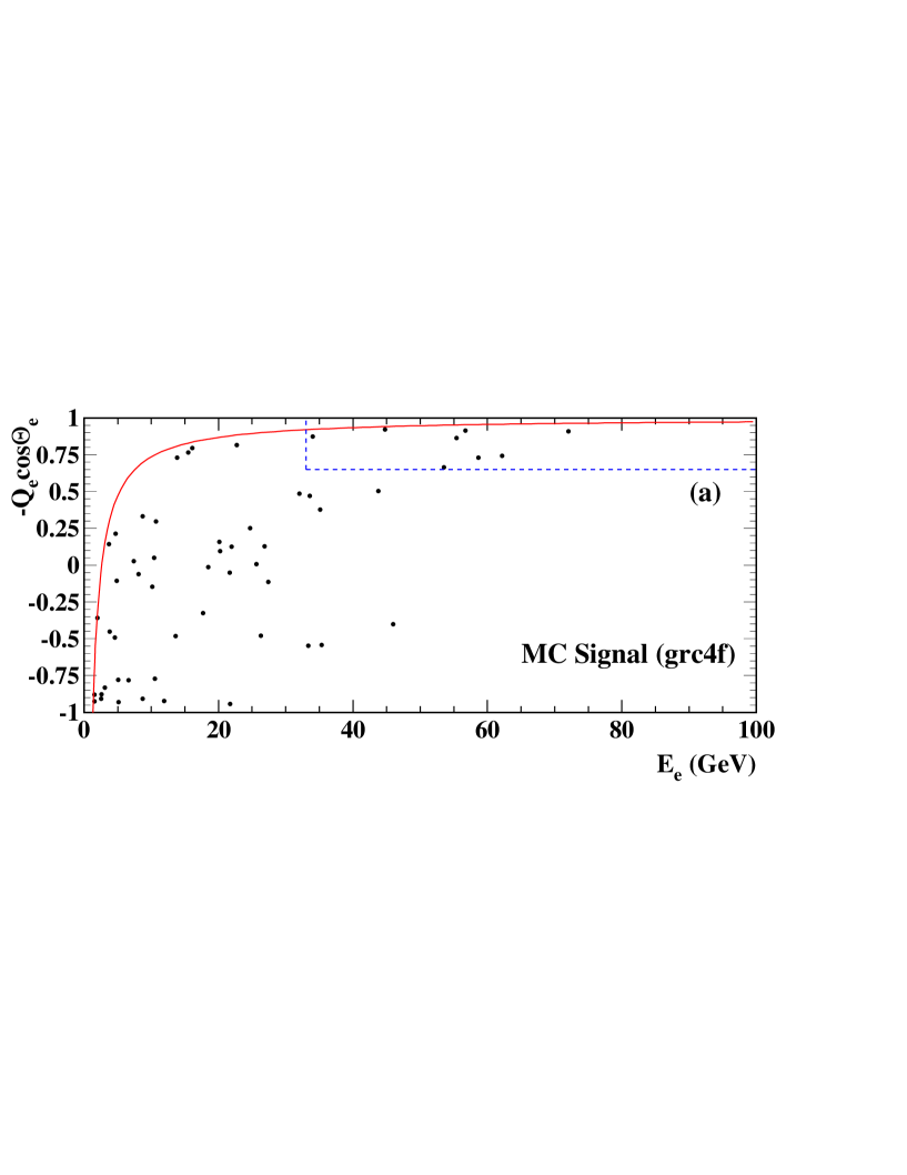
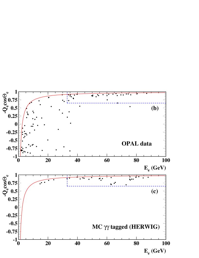
Figure 7: Distribution of the cosine of the scattering angle of the electron $\cos\theta_{\rm e}$ versus its energy $E_{\rm e}$ before the last cut. In (a) the distribution is shown for the signal, in (b) for the data and in (c) for the tagged two-photon Monte Carlo sample. Both Monte Carlo samples have been scaled to the same integrated luminosity as the data. The solid line indicates the cut in the preselection at $|\hat{t}|\geq 500\;\mbox{$\rm GeV$}^{2}$. The area inside the dashed line corresponds to the region discarded by the last selection cut.

In order to remove the remaining background from tagged two-photon reactions those events are rejected where the scattering angle of the electron is in the forward direction by requiring $-\mbox{${\rm Q}_{\rm e}$}\mbox{$\cos\theta_{\rm e}$}\leq 0.65$ or $\mbox{$E_{\rm e}$}\leq 0.35E$. This cut is illustrated in Figure 7.

After all cuts, $70$ events are selected while $68.1\pm 1.9$ events are expected from the Monte Carlo prediction, of which $48.1\pm 1.3$ are signal. This corresponds to an overall signal efficiency of $(15.2\pm 0.4)\%$ according to grc4f. The main contribution to the background stems from tagged two-photon events where one of the scattered electrons is detected within the detector. In the region removed by the last cut the events from two-photon processes are dominant, as shown in Figure 7. For the region outside this cut, the ${\rm Z}/\gamma^{*}{\rm ee}$ events are dominant, but still a non negligible contribution from tagged two-photon events remains.

The cross-section $\sigma_{\rm ee}$ is measured in two different regions of $m_{\rm q\bar{q}}$, in the low invariant mass region ${\rm\gamma^{*}ee}$ and in the high invariant mass region ${\rm Zee}$. By separating the two mass regions at a point where the measured cross-section is near its minimum, the expected feed-through, i.e. the number of events with a true value of $m_{\rm q\bar{q}}$ outside the region it is measured in, is very small. The results of the cross-section measurement for both grc4f and PYTHIA are summarised in Table 3. The efficiency for the high mass region is about 50% larger than that for the low mass region and the expected number of signal events is similar. In the low mass region the background is higher, stemming mainly from tagged two-photon events.

	grc4f		PYTHIA
	${\rm\gamma^{*}ee}$	${\rm Zee}$	${\rm\gamma^{*}ee}$	${\rm Zee}$
Efficiency in $\%$	$13.2\pm 0.5$	$18.0\pm 0.6$	$14.4\pm 0.7$	$19.4\pm 0.8$
Expected signal	$22.7\pm 0.9$	$25.4\pm 0.9$	$26.0\pm 1.5$	$30.2\pm 1.6$
Expected background	$12.1\pm 1.1$	$7.9\pm 0.8$	$12.1\pm 1.1$	$7.9\pm 0.8$
Feed through in $m_{\rm q\bar{q}}$	$0.1\pm 0.1$	$0.2\pm 0.1$	$0.1\pm 0.1$	$0.3\pm 0.2$
OPAL data	$40$	$30$	$40$	$30$
Measured cross-section in pb	$1.20\pm 0.28$	$0.69\pm 0.18$	$1.11\pm 0.26$	$0.64\pm 0.17$
Predicted cross-section in pb	$0.98\pm 0.01$	$0.80\pm 0.01$	$1.03\pm 0.02$	$0.88\pm 0.02$

Table 3: Comparison of OPAL data with the cross-section $\sigma_{\rm ee}$ predicted by the grc4f and the PYTHIA Monte Carlo generator. The errors are statistical only.

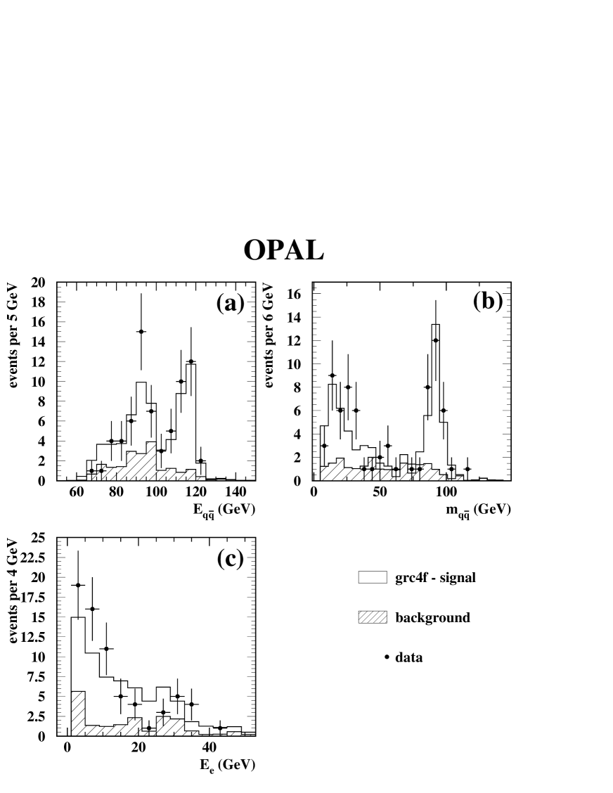
Figure 8: Number of events measured after applying all cuts as a function of (a) the energy $E_{\rm q\bar{q}}$ and (b) mass $m_{\rm q\bar{q}}$ of the quark system and of (c) the electron energy $E_{\rm e}$. The open histogram shows the signal simulated with the grc4f Monte Carlo, the hatched histogram shows the backgrounds from various Monte Carlo simulations and the points the data. Only statistical errors are shown.

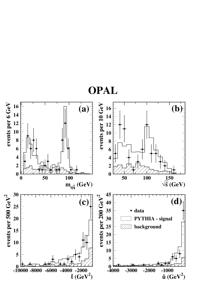
Figure 10: Distribution of (a) the mass $m_{\rm q\bar{q}}$ and the kinematic invariants (b) $\sqrt{\hat{s}}$, (c) $\hat{t}$ and (d) $\hat{u}$ after all cuts. The open histogram shows the signal simulated with the PYTHIA Monte Carlo, the hatched histogram shows the backgrounds from various Monte Carlo simulations and the points the data. Only statistical errors are shown.

In Figures 8 and  9 the measured event distributions for several variables are compared to the ones predicted from the grc4f Monte Carlo simulations. For comparison the event distributions from PYTHIA are given in Figure 10 for some variables. The limited statistics of the data does not allow to distinguish between the two simulations.

6 Determination of differential cross-sections

To compare the results of this analysis with results from other experiments, differential cross-sections are calculated from the distributions of the event variables. For the observed process differential cross sections d$\sigma_{\rm ee}$ and d$\hat{\sigma}_{{\rm e}\gamma}$ have been determined.

6.1 Differential cross-sections d$\sigma_{\rm ee}$

For the determination of the differential cross-sections the experimental resolution is of importance. If the experimental resolution is much smaller than the chosen bin width and the distribution is flat, then the correlation matrix will be close to the unit matrix. But if the distribution is peaked, like for $m_{\rm q\bar{q}}$  then a large fraction of events measured in bins around the peak originated from bins other than the one they had been generated in. Therefore the correlation for each variable between the generated and the measured distribution has to be determined.

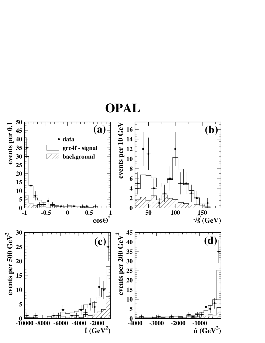
Figure 9: Distribution of (a) the scattering angle in the e$\gamma$ rest-frame $\cos\theta^{*}$, and the kinematic invariants (b) $\sqrt{\hat{s}}$, (c) $\hat{t}$ and (d) $\hat{u}$ after all cuts. The open histogram shows the signal simulated with the grc4f Monte Carlo, the hatched histogram shows the backgrounds from various Monte Carlo simulations and the points the data. Only statistical errors are shown.

The correlation matrix $M$ between the generated and the measured distribution has been calculated for each variable shown in Figures 8 and 9 using the bin width shown there. The matrix $M$ is given by:

$$M(i,j)=\frac{G(i,j)}{\sum_{j}G(i,j)}$$ (11)

and fulfils the following condition:

$$N_{gen}(i)=\sum_{j}M(i,j)N_{det}(j),$$ (12)

where $N_{gen}(i)$ is the number of events generated in bin $i$, $N_{det}(j)$ is the number of events measured in bin $j$ and $G(i,j)$ is the number of events generated in bin $i$ and measured in bin $j$. The matrix $M$ has been determined using the grc4f MC. For most variables $M$ is very similar to the unit matrix with some small off-diagonal elements. For $m_{\rm q\bar{q}}$ around the Z-mass non zero elements exist also away from the first off-diagonal.

The matrix $M$ has also been calculated from the PYTHIA signal MC and no significant difference with the one determined from grc4f has been observed.

The differential cross sections are then given by

$$\frac{{\rm d}\sigma_{\rm ee}}{{\rm d}\,x}=\sum_{j}M(i,j)\left(N_{det}(j,x)-N_{back}(x)\right)\frac{1}{\Delta x}\frac{1}{{\cal L}_{\rm ee}\;\,\epsilon(x)}\ ,$$ (13)

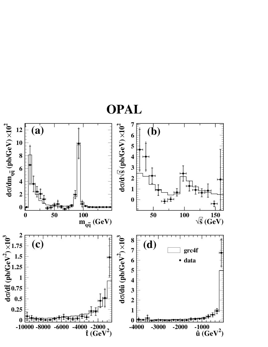
Figure 11: The differential cross-sections (a) $\mathrm{d}\sigma_{ee}/\mathrm{d}m_{{\rm q}\bar{\rm q}}$, (b) $\mathrm{d}\sigma_{ee}/\mathrm{d}\sqrt{\hat{s}}$, (c) $\mathrm{d}\sigma_{ee}/\mathrm{d}\hat{t}$ and (d) $\mathrm{d}\sigma_{ee}/\mathrm{d}\hat{u}$ are shown. The open histograms show the signal simulated with the grc4f Monte Carlo generator and the points the data. The errors show the statistical and systematic errors added in quadrature. The contribution of the statistical errors is indicated by the horizontal bars.

where $x$ is the variable used, ${\cal L}_{\rm ee}$ the integrated luminosity and $\epsilon(x)$ the efficiency in a given $x$ bin. The differential cross-sections are shown in Figure 11.

6.2 Differential cross-sections d$\hat{\sigma}_{{\rm e}\gamma}$

A further aim of this analysis is to calculate the differential cross-sections d$\hat{\sigma}_{{\rm e}\gamma}$. This allows the results from a given ${\rm e}^{+}{\rm e}^{-}$ centre-of-mass energy to be compared with other energies as well as with results from other colliders. To calculate the differential cross-section for a variable $x$, Equation 1 has to be inverted:

$$\frac{{\rm d}\hat{\sigma}_{{\rm e}\gamma}}{{\rm d}\,x}=\frac{1}{\Delta z}\;\;\frac{1}{\mbox{$D_{{\rm e}\gamma}(z,\mbox{$\hat{u}$})_{\overline{\rm\rm EPA}}$}}\;\;\frac{{\rm d}\sigma_{\rm ee}}{{\rm d}\,x},$$ (14)

with $D_{{\rm e}\gamma}(z,\mbox{$\hat{u}$})_{\overline{\rm\rm EPA}}$ being the photon-flux and $\Delta z=\Delta\mbox{$\hat{s}$}/s$. The lower limit of $\sqrt{\mbox{$\hat{s}$}}$ is given by the signal definition as 23 GeV and the upper limit is 160 GeV, resulting in $\Delta z=0.702$. To calculate ${\rm d}\hat{\sigma}_{{\rm e}\gamma}/{\rm d}\,x$ the mean of the inverse of the photon-flux $<1/\mbox{$D_{{\rm e}\gamma}(z,\mbox{$\hat{u}$})_{\overline{\rm\rm EPA}}$}>$ is calculated in bins of $\hat{u}$ and $\hat{s}$. Taking into account the dependence of $<1/\mbox{$D_{{\rm e}\gamma}(z,\mbox{$\hat{u}$})_{\overline{\rm\rm EPA}}$}>$ on $\hat{u}$ is necessary, as the efficiency varies with $\hat{u}$. We have chosen three bins in $\hat{u}$ and four in $\hat{s}$. The bin boundaries as well as the mean values of $<1/\mbox{$D_{{\rm e}\gamma}(z,\mbox{$\hat{u}$})_{\overline{\rm\rm EPA}}$}>$ are given in Table 4. The dependence of $<1/\mbox{$D_{{\rm e}\gamma}(z,\mbox{$\hat{u}$})_{\overline{\rm\rm EPA}}$}>$ on $\hat{u}$ is small while it is large for $\hat{s}$. The width of the bins is chosen to be at least three times larger than the experimental resolution.

		bins in $\hat{u}$ in GeV2
$\bigg{<}\frac{1}{\mbox{$D_{{\rm e}\gamma}(z,\mbox{$\hat{u}$})_{\overline{\rm\rm EPA}}$}}\bigg{>}$		$-50000$ to $-1000$	$-1000$ to $-200$	$-200$ to $-10$
bins	$23$ to $50$	$0.69$	$0.67$	$0.59$
in $\sqrt{\mbox{$\hat{s}$}}$	$50$ to $80$	$2.02$	$2.03$	$2.24$
in GeV	$80$ to $110$	$6.08$	$6.61$	$7.19$
	$110$ to $160$	$13.90$	$14.49$	$16.06$

Table 4: Mean values of the inverse of the photon flux $<1/\mbox{$D_{{\rm e}\gamma}(z,\mbox{$\hat{u}$})_{\overline{\rm\rm EPA}}$}>$ in bins of $\hat{u}$ and $\sqrt{\mbox{$\hat{s}$}}$.

The differential cross-section d$\sigma_{\rm ee}$/d$x$ is calculated according to Equation 13 using bins of $\hat{u}$ and $\hat{s}$.

$$\frac{{\rm d}\sigma_{\rm ee}}{{\rm d}\,x}=\sum_{\mbox{$\hat{u}$},\mbox{$\hat{s}$}}\frac{N(\mbox{$\hat{s}$},\mbox{$\hat{u}$},x)/\Delta x}{{\cal L}_{\rm ee}\;\,\epsilon(\mbox{$\hat{u}$},x)}\ ,$$ (15)

where $N(\mbox{$\hat{s}$},\mbox{$\hat{u}$},x)$ is the number of events in bins of $\hat{s}$, $\hat{u}$ and $x$ after subtracting the background and using the matrix $M$. Larger bins compared to the previous section have been used and $M$ is calculated using these bin sizes. The efficiency $\epsilon(\mbox{$\hat{u}$},x)$ is calculated only in bins of $\hat{u}$ and $x$ as it is flat in $\sqrt{\mbox{$\hat{s}$}}$. This results in the differential cross-section in the ${\rm e}\gamma$ system to be given by:

$$\frac{{\rm d}\hat{\sigma}_{{\rm e}\gamma}}{{\rm d}\,x}=\sum_{\mbox{$\hat{u}$},\mbox{$\hat{s}$}}\frac{N(\mbox{$\hat{s}$},\mbox{$\hat{u}$},x)/\Delta x}{{\cal L}_{\rm ee}\;\,\epsilon(\mbox{$\hat{u}$},x)}\;\,\frac{1}{\Delta z}\;\,\bigg{<}\frac{1}{\mbox{$D_{{\rm e}\gamma}(z,\mbox{$\hat{u}$})_{\overline{\rm\rm EPA}}$}}\bigg{>}\;.$$ (16)

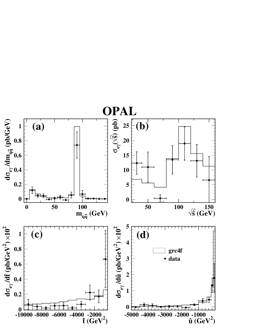
Figure 12: The differential cross-sections (a) d$\hat{\sigma}_{{\rm e}\gamma}$/$\mathrm{d}m_{{\rm q}\bar{\rm q}}$, (c) d$\hat{\sigma}_{{\rm e}\gamma}$$/\mathrm{d}\hat{t}$ and (d) d$\hat{\sigma}_{{\rm e}\gamma}$$/\mathrm{d}\hat{u}$ are shown. In addition (b) the cross section $\hat{\sigma}_{{\rm e}\gamma}$$(\sqrt{\hat{s}})$ is shown The open histograms show the signal simulated with the grc4f Monte Carlo generator and the points the data. The errors show the statistical and systematic errors added in quadrature. The contribution of the statistical errors is indicated by the horizontal bars.

The measured differential cross-sections are shown in Figure 12 and are compared to the generated distributions.

For calculating the total cross-section $\hat{\sigma}_{{\rm e}\gamma}$$(\sqrt{\mbox{$\hat{s}$}})$ as a function of $\sqrt{\mbox{$\hat{s}$}}$ the same method as above is applied, with the difference that $\Delta z$ is calculated for each bin of $\sqrt{\mbox{$\hat{s}$}}$.

7 Systematic error studies

For the calculation of the total and differential cross-sections the efficiencies, unfolding matrix and backgrounds are taken from Monte Carlo simulations. It is therefore important to study systematic effects resulting from these simulations.

7.1 Systematic error studies for the total cross-section

The systematic errors on the efficiencies come mainly from imperfect modelling of the detector response. This can lead to discrepancies between the data and the Monte Carlo simulation in the distributions of the cut variables. These systematic errors can be estimated, for example, by comparing Monte Carlo simulation and data.

This has been done using the events selected by the preselection. For these events each of the selection cuts has been applied separately and the relative difference in the number of events selected in data and in Monte Carlo has been assigned as a systematic error after quadratically subtracting the statistical error. In cases where this results in a value being lower than the statistical error, conservatively the statistical error is used. An error common for the whole mass range has been calculated and no distinction between the low and high mass range has been made. The values of the errors are listed in Table 5. These systematic uncertainties are used for both the ${\rm\gamma^{*}ee}$-like and ${\rm Zee}$-like kinematic regions since the efficiencies of each of these selection cuts are similar in the two regions.

As a cross check the systematic errors have also been estimated by comparing Monte Carlo simulation and data for the process $\rm{W^{+}W^{-}}\rightarrow\rm{qq}{\rm e}{\nu}_{\rm e}$ which has the same observable final state as the ${\rm Z}/\gamma^{*}{\rm ee}$ process. $\rm{W^{+}W^{-}}\rightarrow\rm{qq}{\rm e}{\nu}_{\rm e}$ events are selected according to the procedure described in [26] and then each selection cut is applied separately to this sample. For those cuts where the distribution of the cut variables is similar for $\rm{W^{+}W^{-}}\rightarrow\rm{qq}{\rm e}{\nu}_{\rm e}$, ${\rm Zee}$ and ${\rm\gamma^{*}ee}$ events (the absolute value of the missing momentum, the electron isolation and the electron angle and energy) no difference within the statistical error in the systematic error compared to the method described above has been observed.

The relatively smaller overall efficiency for ${\rm\gamma^{*}ee}$-like events arises mainly from the multiplicity cut in the preselection. To asses the systematic uncertainty of this cut the number of tracks and clusters required has been changed by $\pm 1$.

	${\rm\gamma^{*}ee}$	${\rm Zee}$
multiplicity	0.024	—
$\mbox{$|p_{\rm miss}|$}\geq 35$ GeV	0.042	0.042
electron isolation	0.038	0.038
$-\mbox{${\rm Q}_{\rm e}$}\mbox{$\cos\theta_{\rm e}$}$ cut	0.028	0.028
$\mbox{${\rm Q}_{\rm e}$}\mbox{$\cos\theta_{\rm miss}$}\geq 0.95$	0.033	0.033
$\mbox{${E}_{\rm fwd}$}\leq 30$ GeV	0.056	0.056
detector simulation	0.094	0.091
efficiency	0.049	0.050
background	0.038	0.033
Total	0.113	0.109

Table 5: Relative systematic uncertainties of the cross-section measurements. The entry “detector simulation” is the quadratic sum of the signal efficiency uncertainties for the single cuts listed in the rows above it.

The uncertainty in the efficiency due to the choice of a particular Monte Carlo event generator is estimated by comparing PYTHIA and grc4f. For this comparison only events with the signal electron within the acceptance of the detector, defined by a cut on generator level on the angle of the electron $|\cos\theta_{\rm e}^{\rm{gen}}|\leq 0.963$ are used. The relative difference in efficiency of the two different Monte Carlo generators after subtracting the statistical errors quadratically is taken as a systematic error.

Uncertainties affecting the residual background have been evaluated separately for each of the three main background classes remaining after all cuts. Background-enriched samples are obtained by inverting or omitting one or two cuts, while the other cuts remain unchanged. The full difference between the number of events remaining in the data and the number of expected events from Monte Carlo is taken as a systematic uncertainty. For the background from four-fermion final states the cut on the fit probability is omitted and the cut on the electron isolation is inverted. After applying these cuts, a relative difference of $17\%$ between the data and Monte Carlo is observed. The background from tagged two-photon events is enriched by inverting the cut on the electron’s angle and energy. The relative systematic error is $10\%$. By omitting the cut on the angle of the missing momentum and inverting the electron isolation cut the multi-hadronic background is enriched, leading to a relative systematic uncertainty of $12\%$.

The numbers of background events after all cuts in the ${\rm\gamma^{*}ee}$ region are $4.47\pm 0.39\pm 0.75$ from four fermion events, $1.07\pm 0.19\pm 0.11$ from multi-hadronic processes and $5.80\pm 1.01\pm 0.73$ events from tagged two-photon reactions. In the Zee region the corresponding contributions are $3.81\pm 0.34\pm 0.64$, $1.38\pm 0.22\pm 0.14$ and $2.46\pm 0.66\pm 0.31$ events. Additional background sources contribute with less than $1$ event for each mass region. This leads to a relative error on the cross-section of $3.8\%$ in the low mass region and $3.3\%$ in the high mass region, as quoted in Table 5.

In further studies contributions to the background not modelled in the Monte Carlo were investigated. Using random beam-crossing events, the interactions between the beam particles and the gas inside the vacuum pipe were found to be negligible.

For the multi-hadronic background an additional systematic cross-check is applied by comparing the prediction of two different Monte Carlo generators. A good agreement between the PYTHIA and YFS3FF Monte Carlo generators has been found within the statistical errors. Consequently no additional systematic error has been assigned.

7.2 Systematic error studies for the differential cross-sections

The systematic errors for the differential cross-sections stem mainly from the imperfect detector simulation in the Monte Carlo and from the uncertainty in the unfolding matrix $M$.

The error assigned for the detector simulation is taken to be the same as for the total cross-section. A value of 9.4% is assigned. The unfolding matrix $M$ is calculated using both the grc4f and the PYTHIA Monte Carlo sample and the relative difference between the two is taken as a systematic error. For the background the same errors as determined for the total cross-section are used. The errors for the three different background classes are taken into account in each bin of the event distributions. The efficiency $\epsilon$ is calculated in bins of the variable $x$ for the differential cross-sections d$\sigma_{\rm ee}$ and in bins of $\hat{u}$ and the variable $x$ for the differential cross-sections d$\hat{\sigma}_{{\rm e}\gamma}$. It has therefore much larger statistical errors than in the calculation of the total cross section. Within the statistical errors no difference between the efficiencies determined from the grc4f and the PYTHIA Monte Carlo samples has been observed. Consequently no systematic error has been assigned.

Due to the small statistics of the data sample the systematic error for the differential cross-sections is much smaller than the statistical one.

8 Results and discussion

The cross-section for the process $\mbox{${\rm e}^{+}{\rm e}^{-}$}\to{\rm\mbox{${\rm e}^{+}{\rm e}^{-}$}Z}/\gamma^{*}$ has been measured in a restricted phase space, defined by Lorentz invariant variables, in two different regions of the mass of the hadronic system, corresponding to either a $\gamma^{*}$ or a Z⁰ in the final state. With the cut at $m_{\rm q\bar{q}}$ = $60$ GeV the $\gamma^{*}$ and the Z⁰ are well separated. With an integrated luminosity of about $175$ pb^-1, a total of $70$ candidate events have been observed, while $20.0\pm 1.4$ background events and $48.1\pm 1.3$ signal events are predicted, giving a total of $68.1\pm 1.9$ events. The cross-sections times branching ratio for the decay of ${\rm Z}/\gamma^{*}$ into hadrons, $\sigma_{\rm ee}$, are found to be $\sigma=(1.20\pm 0.28\pm 0.14)$ pb for ${\rm\gamma^{*}ee}$ and $\sigma=(0.69\pm 0.18\pm 0.08)$ pb for ${\rm Zee}$ final states within the kinematical definition listed in Table 1. A large part of this cross-section is not detectable within the detector as the scattering angle of the electron is in the very backward direction. For the calculation of the cross-sections the efficiencies predicted by the grc4f generator are used. The cross-sections measured using efficiencies predicted by PYTHIA lie well within the errors.

The distributions of $E_{\rm q\bar{q}}$, $m_{\rm q\bar{q}}$and $E_{\rm e}$ are shown in Figures 8(a) to (c), respectively. The distribution of $E_{\rm q\bar{q}}$ shows two peaks, one at the beam energy and one at about $115$ GeV. From equation 9 one obtains for the largest part of the cross-section at $\hat{u}=0$ and $Q_{e}\cos\theta_{{\rm q}\bar{\rm q}}=-1$

$$E_{{\rm q}\bar{\rm q}}=E_{\rm beam}+\frac{m_{\rm q\bar{q}}^{2}}{4E_{\rm beam}}.$$ (17)

Consequently, the peak at the beam energy corresponds to ${\rm\gamma^{*}ee}$ and the peak at $115$ GeV to the ${\rm Zee}$ process. The tail at lower energies is due to the parts of the cross-section where $\hat{u}\neq 0$ and $Q_{e}\cos\theta_{{\rm q}\bar{\rm q}}\neq-1$. Two peaks are visible in the invariant mass distribution, stemming from the contributions of the two gauge bosons, the $\gamma^{*}$ and the Z. The expected background is flat over the whole mass range up to 100 GeV. For both distributions the shapes of Monte Carlo and data are in good agreement. The two Monte Carlo generators give similar distributions and more statistics is needed to distinguish between the two.

In Figure 9 the distributions of the scattering angle $\theta^{*}$ of the ${\rm Z}/\gamma^{*}$ in the e$\gamma$ rest-system with respect to the incoming photon direction, as well as the distribution of the kinematic invariants $\sqrt{\hat{s}}$, $\hat{t}$ and $\hat{u}$ are shown and are compared with the predictions of grc4f. The scattering angle $\theta^{*}$ peaks strongly in the backward direction and the agreement between data and Monte Carlo is good. The observed structure of the distribution of $\sqrt{\hat{s}}$, can be understood in terms of the ${\rm\gamma^{*}ee}$ final states in the low $\sqrt{\hat{s}}$ region and the ${\rm Zee}$ in the high $\sqrt{\hat{s}}$ region. In Figure 10 the measured distributions are compared to the distributions from PYTHIA. The predictions of both grc4f and PYTHIA are in agreement with the data. The distribution of $\hat{t}$ is peaked towards $0$ and shows a long tail towards large values. The distribution of $\hat{u}$ shows the typical behaviour of a $u$-channel process, a peak at zero.

From these event distributions the differential cross-sections d$\sigma_{\rm ee}$ are derived and are shown in Figure 11. Only Lorentz invariant quantities have been derived. The Monte Carlo describes the data well, except for small values of $\sqrt{\hat{s}}$, where the Monte Carlo underestimates the data. In the distribution of $\mathrm{d}\sigma_{ee}/\mathrm{d}m_{{\rm q}\bar{\rm q}}$ for small values of $m_{\rm q\bar{q}}$ the steep falloff of the cross-section with increasing invariant mass $m_{\rm q\bar{q}}$ as well the peak at the Z-mass are very well visible. The distribution of $\mathrm{d}\sigma_{ee}/\mathrm{d}\sqrt{\hat{s}}$ shows a decrease with increasing $\sqrt{\hat{s}}$ until the threshold for Z Boson production is reached.

From the differential cross-sections d$\sigma_{\rm ee}$ the differential cross-sections for the sub-process $\mbox{${\rm e}\gamma$}\to\mathrm{e}$ ${\rm Z}/\gamma^{*}$  are deduced, based on a factorisation ansatz using the modified Equivalent Photon approximation from Equation 5. They are shown in Figure 12.

The distribution of d$\mbox{$\hat{\sigma}_{{\rm e}\gamma}$}/\rm{d}m_{\rm{qq}}$ shows a strong peak around the Z Boson mass. The differential cross-section d$\hat{\sigma}_{{\rm e}\gamma}$/d$\hat{u}$ shows a very sharp peak at 0, as expected for this $u$-channel process. For d$\hat{\sigma}_{{\rm e}\gamma}$/d$\hat{t}$ the Monte Carlo does not describe the data so well. The increase for $\hat{t}$ towards 0 is well reproduced, but for large negative values of $\hat{t}$ the Monte Carlo lies constantly above the data.

In Figure 12(b) the total cross-section $\hat{\sigma}_{{\rm e}\gamma}$($\sqrt{\mbox{$\hat{s}$}}$) is shown. Note the dip in the cross-section at $\sqrt{\mbox{$\hat{s}$}}$ around 70 GeV. The total cross-section $\hat{\sigma}_{{\rm e}\gamma}$($\sqrt{\mbox{$\hat{s}$}}$) shows a decrease with increasing $\sqrt{\hat{s}}$ until the threshold for Z Boson production is reached. This is the first measurement of $\hat{\sigma}_{{\rm e}\gamma}$($\sqrt{\mbox{$\hat{s}$}}$) around the Z Boson threshold. $\hat{\sigma}_{{\rm e}\gamma}$($\sqrt{\mbox{$\hat{s}$}}$) is independent of the ${\rm e}^{+}{\rm e}^{-}$ centre-of-mass energy and can therefore be compared with measurements at other ${\rm e}^{+}{\rm e}^{-}$ centre of mass energies as well with measurements at other colliders, e.g. HERA.

Within the statistical error, the Monte Carlo predictions are in good agreement with the data. But there is a tendency that the data are higher than the Monte Carlo in the low $\sqrt{\hat{s}}$ region, while they are too low in the high $\sqrt{\hat{s}}$ region.

9 Conclusions

The process $\mbox{${\rm e}^{+}{\rm e}^{-}$}\to{\rm\mbox{${\rm e}^{+}{\rm e}^{-}$}Z}/\gamma^{*}$ and its subprocess ${\rm e}\gamma\to{\rm eZ}/\gamma^{*}$ have been studied. For the process $\mbox{${\rm e}^{+}{\rm e}^{-}$}\to{\rm\mbox{${\rm e}^{+}{\rm e}^{-}$}Z}/\gamma^{*}$ the cross-section times branching ratio for the decay of the ${\rm Z}/\gamma^{*}$ into hadrons at $\sqrt{s}=189$ GeV has been measured within a restricted phase space to be $\sigma=(1.20\pm 0.28\pm 0.14)$ pb for $m_{\rm q\bar{q}}$$<60$ GeV and $\sigma=(0.69\pm 0.18\pm 0.08)$ pb for $m_{\rm q\bar{q}}$$\geq 60$ GeV. The Monte Carlo generators grc4f and PYTHIA both predict cross-sections within one standard deviation of the measured values. The cross-section $\hat{\sigma}_{{\rm e}\gamma}$($\sqrt{\mbox{$\hat{s}$}}$) for the subprocess ${\rm e}\gamma\to{\rm eZ}/\gamma^{*}$ has been determined in a range of $\sqrt{\mbox{$\hat{s}$}}$ from 23 to 160 GeV.

Differential cross-sections d$\sigma_{\rm ee}$ and d$\hat{\sigma}_{{\rm e}\gamma}$ have been determined and compared to the ones from the Monte Carlo generators grc4f and PYTHIA. The generators describe all distributions well.

Acknowledgements

The authors would like to thank T. Sjöstrand for his help by making the changes to PYTHIA necessary to describe the process investigated in this paper.

We particularly wish to thank the SL Division for the efficient operation of the LEP accelerator at all energies and for their continuing close cooperation with our experimental group. We thank our colleagues from CEA, DAPNIA/SPP, CE-Saclay for their efforts over the years on the time-of-flight and trigger systems which we continue to use. In addition to the support staff at our own institutions we are pleased to acknowledge the
Department of Energy, USA,
National Science Foundation, USA,
Particle Physics and Astronomy Research Council, UK,
Natural Sciences and Engineering Research Council, Canada,
Israel Science Foundation, administered by the Israel Academy of Science and Humanities,
Minerva Gesellschaft,
Benoziyo Center for High Energy Physics,
Japanese Ministry of Education, Science and Culture (the Monbusho) and a grant under the Monbusho International Science Research Program,
Japanese Society for the Promotion of Science (JSPS),
German Israeli Bi-national Science Foundation (GIF),
Bundesministerium für Bildung und Forschung, Germany,
National Research Council of Canada,
Research Corporation, USA,
Hungarian Foundation for Scientific Research, OTKA T-029328, T023793 and OTKA F-023259.

Figure 1: Diagrams for the process $\mbox{${\rm e}^{+}{\rm e}^{-}$}\to{\rm(e)e}\mbox{${\rm Z}/\gamma^{*}$}$.

(a)                                                  (b)

Figure 2: Further diagrams leading to the final state eeqq. On the left is the multiperipheral diagram and on the right is the conversion diagram.

Figure 3: Distribution of the charge weighted cosine of the scattering angle of the electron $-$${\rm Q}_{\rm e}$$\cos\theta_{\rm e}$ versus its energy $E_{\rm e}$ as predicted by the grc4f signal Monte Carlo at generator level. The solid line corresponds to $|\hat{t}|=500\;\mbox{$\rm GeV$}^{2}$.

Figure 4: Distribution of the transverse momentum $\hat{p}_{t}$ of the ${\rm Z}/\gamma^{*}$  in the e$\gamma$ rest-frame, the hadronic mass, $m_{\rm q\bar{q}}$, the electron energy, E_e, and $\hat{t}$ at generator level for the signal for all events fulfilling the signal definition. The histograms show the distributions for the grc4f sample and the points for the PYTHIA sample. Only the statistical errors of the PYTHIA sample are shown. The distributions are normalised to the data luminosity.

Figure 5: Distribution of (a) $m_{\rm q\bar{q}}$ and (b) the electron energy $E_{\rm e}$ after the preselection. The histograms show the contributions from the various processes and the points represent the data. The signal contribution is taken from the grc4f Monte Carlo sample. Only statistical errors are shown.

Figure 6: Distributions of variables used in cuts in the preselection and in the selection. (a) $P$, the fit probability, (b) $p_{\mathrm{miss}}$, the missing momentum, (c) the angle between the electron track and the nearest track, and (d) $E_{FWD}$, the energy deposited in the forward calorimeter before applying the cut on that variable. The arrows indicate the selected region. Only statistical errors are shown. The histograms show the contributions from the various processes and the points represent the data.

References

- [1] OPAL Collaboration, G. Abbiendi et al., Phys. Lett. B438 (1998) 391.
-
[2]
G. Altarelli, G. Martinelli, B. Mele and R. Rückl,
Nucl. Phys. B262 (1985) 204;
E. Gabrielli, Mod. Phys. Lett. A1 (1986) 465. - [3] K. Hagiwara et al., Nucl. Phys. B365 (1991) 544.
- [4] LEP2 Yellow Report, CERN 96-01, Vol1 (1996) 233, and T. Sjöstrand, private communication.
- [5] P. Salati and J.C. Wallet, Z. Phys. C16 (1982) 155.
-
[6]
OPAL Collaboration, K. Ahmet et al., Nucl. Instr. Meth. A305 (1991) 275;
S. Anderson et al., Nucl. Instr. Meth. A403 (1998) 326. - [7] B.E. Anderson et al., IEEE Transactions on Nuclear Science 41 (1994) 845.
- [8] G. Aguillion et al., Nucl. Instr. Meth. A417 (1998) 277.
- [9] S.Y. Choi, Z. Phys. C68 (1995) 163.
- [10] F. Cornet, R. Graciani, J.I. Illana, Granada preprint UG FT 65/96 (1996).
- [11] J. Fujimoto et al., Comp. Phys. Comm. 100 (1997) 128.
- [12] T. Sjöstrand, Comp. Phys. Comm. 82 (1994) 74.
- [13] OPAL Collaboration, G. Alexander et al., Z. Phys. C69 (1996) 543.
- [14] G. Marchesini et al., Comp. Phys. Comm. 67 (1992) 465.
-
[15]
R. Engel, Z. Phys. C66 (1995) 203;
R. Engel and J. Ranft, Phys. Rev. D54 (1996) 4244. -
[16]
R. Bhattacharya, J. Smith and G. Grammer, Phys. Rev. D15 (1977) 3267;
J. Smith, J.A.M. Vermaseren and G. Grammer, Phys. Rev. D15 (1977) 3280;
J.A.M. Vermaseren, Nucl. Phys. B229 (1983) 347. - [17] S. Jadach, W. Placzek, B.F.L. Ward, Phys. Rev. D56 (1997) 6939.
- [18] S. Jadach, B.F.L. Ward and Z. Wa̧s, Comp. Phys. Comm. 79 (1994) 503.
- [19] S. Jadach, W. Placzek and B.F.L. Ward, Phys. Lett. B390 (1997) 298.
- [20] D. Karlen, Nucl. Phys. B289 (1987) 23.
- [21] J. Allison et al., Nucl. Instr. Meth. A317 (1992) 47.
- [22] OPAL Collaboration, K. Ackerstaff et al., Eur. Phys. J. C2 (1998) 213.
- [23] OPAL Collaboration, G. Alexander et al., Z. Phys. C70 (1996) 357.
-
[24]
N. Brown and W.J. Stirling, Phys. Lett. B252 (1990) 657;
S. Bethke, Z. Kunszt, D. Soper and W.J. Stirling, Nucl. Phys. B370 (1992) 310;
S. Catani et al., Nucl. Phys. B269 (1991) 432;
N. Brown and W.J. Stirling, Z. Phys. C58 (1992) 629. - [25] M. Hauschild et al., Nucl. Instr. Meth. A314 (1994) 74.
- [26] OPAL Collaboration, K. Ackerstaff et al., Eur. Phys. J. C1 (1998) 395.
(a) (b)